1. Introduction
The National Water Resources Policy, 9433 Law of 1997 [
1], defines that the management of water resources must always provide the multiple uses of water. From this perspective, the management of the generation of energy by hydropower plants gains great importance in Brazil since it currently represents 64.9% of the Brazilian electric generation matrix [
2].
To guide the conditions and procedures to be observed by concessionaires and authorized hydroelectric power generation in Brazil, a joint rule was published between the National Water Agency (ANA) and the National Electric Energy Agency (ANEEL) [
3] which foresees the need for installation, operation, and maintenance of hydrometric stations aiming at the pluviometric, limnimetric, fluviometric, sedimentometric, and water quality monitoring associated with hydropower plants.
According to the ANA-ANEEL Joint Resolution March 2010 [
3], ANA assumes that the function of guiding the agents of the electric sector on the procedures of collecting, treatment, and storing this hydrometric data, as well as sending this information in a compatible format with the National Water Resources Information System (SNIRH), aims to disseminate data from hydrological monitoring.
It is also important to highlight that government or environmental agencies’ regulations defines the environmental flow methodology conditions to the energy production by hydropower plants. There is a large number of recorded methodologies for environmental flow implementation worldwide [
4]. In Brazil the hydrologically based is adopted. In Brazil’s Federal rivers, which exceed the limit of a State of the country, the environmental flow is defined by the National Water Agency, equal to 70% of the Q95 [
5]. On the other hand, states rivers have the limit of environmental flows defined individually, in which the river belongs and it can be a percentage of a flow duration curve (Q90 or Q95) or 7-day low flow event (Q7,10).
Some studies [
6,
7] demonstrate the strategic importance of regulating a sustainable hydropower operation in the energy production process aiming at maintaining the environmental flow variability, following the natural seasonality of the river flow on the riverine ecosystem. This seasonality in the environmental flow [
8] is important to provide suitable habitat conditions for several river’s species such as fishes or macroinvertebrates community and to mitigating the ecological impacts of hydropower plants. Recently [
9] discussed how changing the natural flow regime due to hydropower operation may affect different aspects of the fluvial ecosystem at a global-scale perspective, based on the literature investigation.
Such rules are extremely important to define criteria and procedures for data collection and knowledge of the hydrological regimes of the basin where the enterprise is located and, thus, allow the definition of operating rules aiming the optimal use of the hydraulic potential of hydropower plants reservoirs.
In this context, the potential of energy of a hydropower plant is directly related to the streamflow of the watercourse. Thus, the technique chosen to conduct hydrometric monitoring became important to plan power generation in Brazil, where the accuracy of the results of field observations depends directly on the technique of measurement adopted.
The recent study developed by [
10] analyzes the current scenario of hydrological monitoring in Brazil and comments on the economic aspects and time costs in campaigns for the acquisition of hydrological data in the field, depending on the type of measurement adopted.
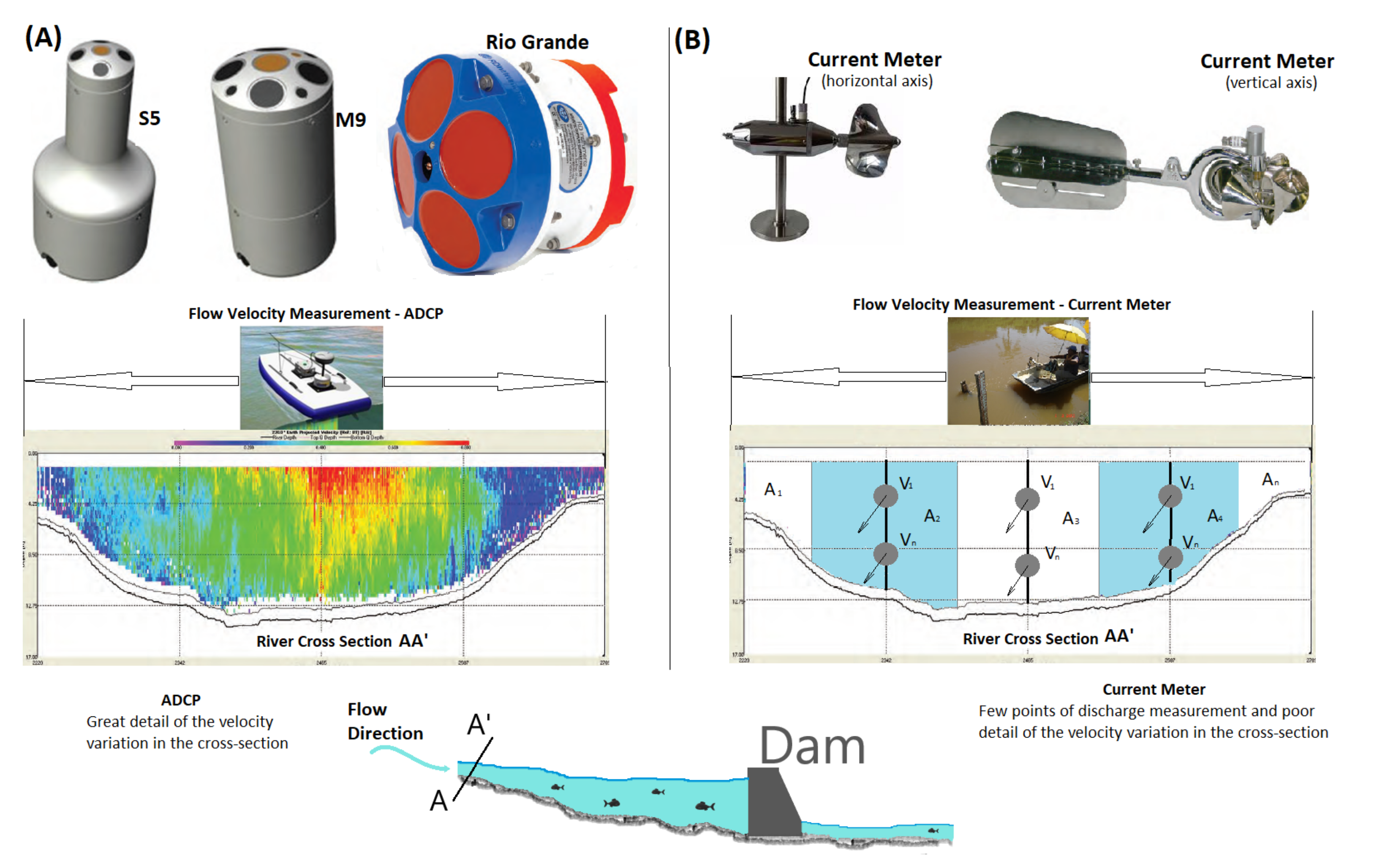
Traditionally, in Brazil, the flows monitoring in gage stations of the national hydrometeorological network is performed by traditional techniques with the Current Meter [
11], in which the cross section of the watercourse is subdivided into several subsections, where point velocities are measured using the Current Meter and the areas of the subsections are obtained by measuring the depth and width of each subsection (
Figure 1B). Integrating these measurements into the width of the watercourse, the streamflow is obtained. However, with increasing technological development and greater reliability in the use of automated techniques for monitoring, the use of ADCP (Acoustic Doppler Current Profiler) has become a reality in Brazil. This equipment uses the principle of the Doppler effect to measure the speed of the water. This technique is known as hydroacoustics (
Figure 1A).
As shown in
Figure 1A, the ADCP has many advantages over the Current Meter Figure shown in
Figure 1B, among which we can mention (a) reduction of the flow measurement time; (b) greater detail of the velocity variation in the cross-section of the watercourse, making a sweep of the velocity distribution, in comparison with the spot measurements of the Current Meter and consequently has a better precision in the flow calculation; (c) possibility of measuring the flow in flood conditions, avoiding putting the hydrometer’s safety at risk [
12].
Several studies were developed to evaluate the accuracy of the different flow measurement methods [
13,
14,
15].
In addition to the precision of the measurement method used to calculate the flow in the field (ADCP or hydrometric vane), the rating curve also has a great influence on the value of the generation of the historical flow series of the fluviometric stations [
16].
Therefore, it is worth noting that the accuracy of the rating curve depends, among other factors, on the accuracy of the flow measurement method adopted. In other words, the calibration of the curve depends on the flow values measured in the field.
Hamilton in [
17] demonstrates that for certain ranges of flow values, the measurement method with ADCP shows better precision in the results.
1.1. The Study Aim: Firm Energy
In Brazil, the sale rules of electricity determine ascertains that each hydropower plant has a generation limit for the establishment of contracts. Due to the fact that hydroelectric generation is strongly influenced by hydrological factors, this limit cannot correspond to the installed capacity of the plant. For a better understanding, some definitions from Brazilian system are necessary, [
18,
19,
20]
Firm Energy of the System: According to the National Power System Operator (ONS), the firm energy of the system can be defined as being the highest possible value of energy capable of being supplied continuously by the system. This supply must occur without any deficit and considering the system configuration and market characteristics constant. It should also be considered a repetition of the flow of the historical record;
Firm Energy of a hydropower Plant: Defined as the contribution of this plant to the system’s firm energy that corresponds to its average production over the critical period;
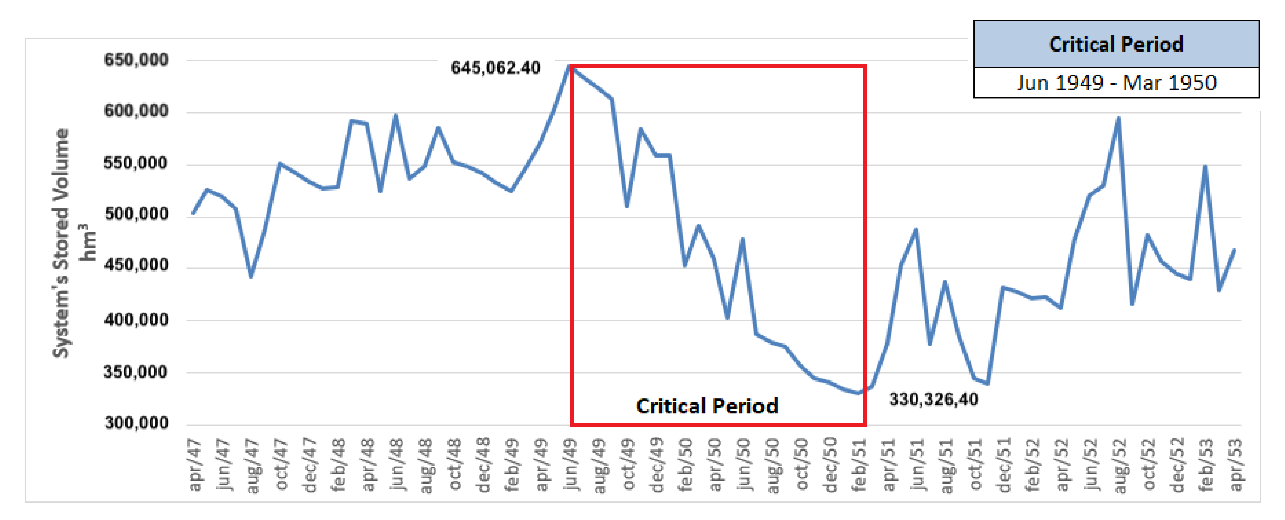
Critical Period: Longer time interval in which the reservoirs of the system’s set of plants are depleted to the maximum. Reservoirs must start full (storage greater than 98% of Maximum Storable Energy) and without intermediate total refills. In addition, the system must be submitted to its firm energy, considering the configuration of its generators, its interconnections and its set of storage reservoirs constant;
Maximum Storable Energy: Defined as the total storage capacity of all reservoirs that compose the system. It can be evaluated as being all the energy produced when the reservoirs of the system are completely depleted (from maximum to minimum storage);
Assured Energy: Defined as the maximum energy production that can be maintained almost continuously by hydropower plants over the years. Therefore, the occurrence of each one of the thousands of possibilities of flow sequences statistically created is simulated, and a certain risk of not meeting the load is admitted, i.e., in a certain percentage of the simulated years, rationing is allowed within a limit considered acceptable by the system. In the current regulation, this risk is 5%. The Assured Energy of a hydropower plant is the fraction allocated to it of the system’s assured energy.
Energy Reallocation Mechanism (MRE): Financial mechanism that aims to share the hydrological risks that affect generators, in the quest to guarantee the optimization of the system’s hydroelectric resources. The purpose is to ensure that all participating generators sell the assured energy that has been allocated to them. Regardless of their actual energy production, as long as the MRE plants, as a whole, have generated enough energy to do so.
The individualized firm energy of hydropower plants is used as a factor to apportion the overall assured energy of a system to the hydropower plants that comprise it. Therefore, we must measure the individual firm energy of a plant, since it directly influences the determination of its assured energy, which is used to establish contracts between distributors, free consumers and traders.
1.2. The Study Place: Itapebi Hydropower Plant
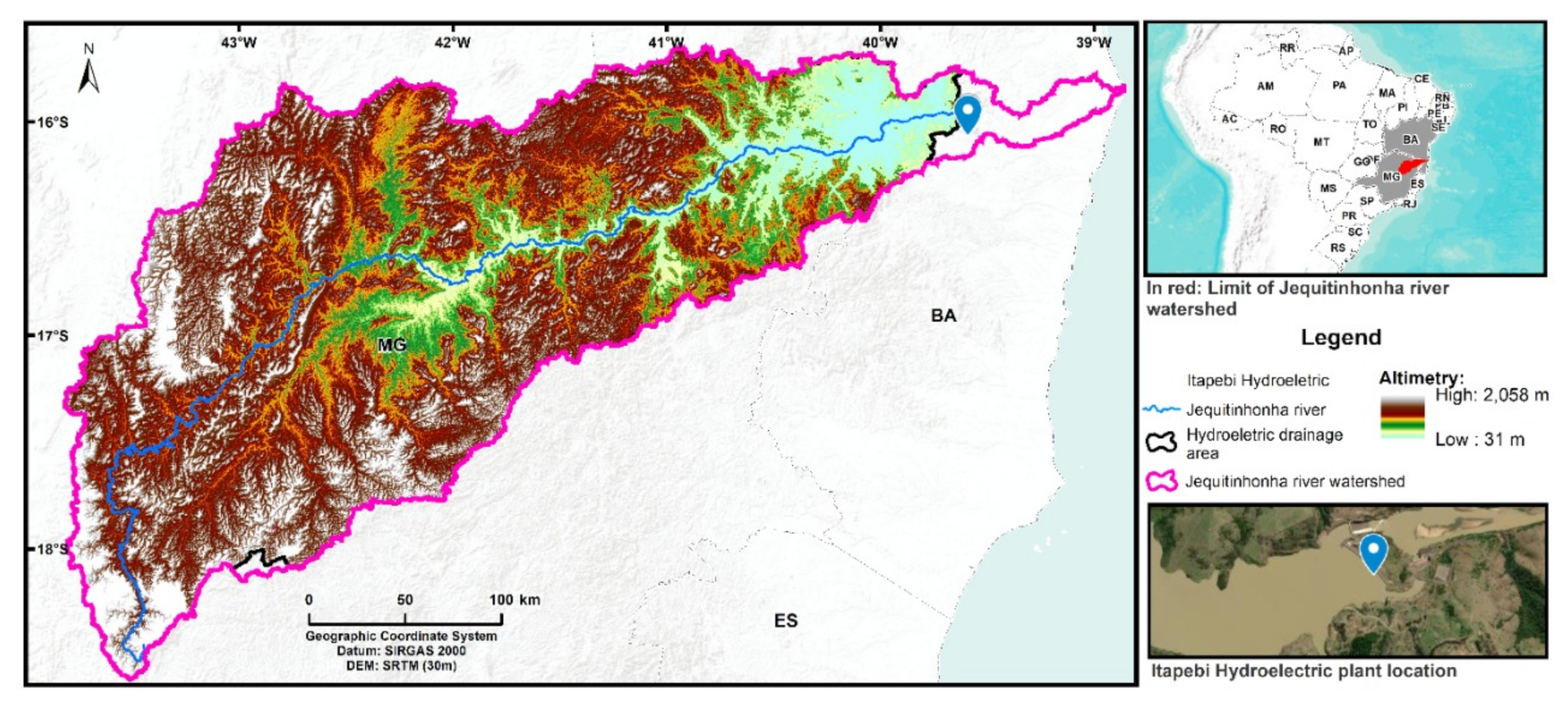
The Itapebi hydropower plant is located in the municipality of Itapebi-BA and belongs to the Jequitinhonha River basin, which has a drainage area of approximately 70,315 km
, 93% of which is within the limits of the State of Minas Gerais (MG) and the rest in southeastern Bahia. The Jequitinhonha River rises in the Serra do Espinhaço, in the municipality of Serro/MG, at an altitude of approximately 1267 m and, after covering about 918 km in length, reaches the dam site of the Itapebi hydropower plant at an altitude of 31 m. The main tributaries of the Jequitinhonha River are the Itacambiruçu, Salinas, São Pedro, and São Francisco rivers on the left bank, and Araçuaí, Piauí and São Miguel, on the right bank, as shown in
Figure 2.
1.3. The Study Contributions
To validate the importance of an accurate measurement of inflow values, this work has two main objectives:
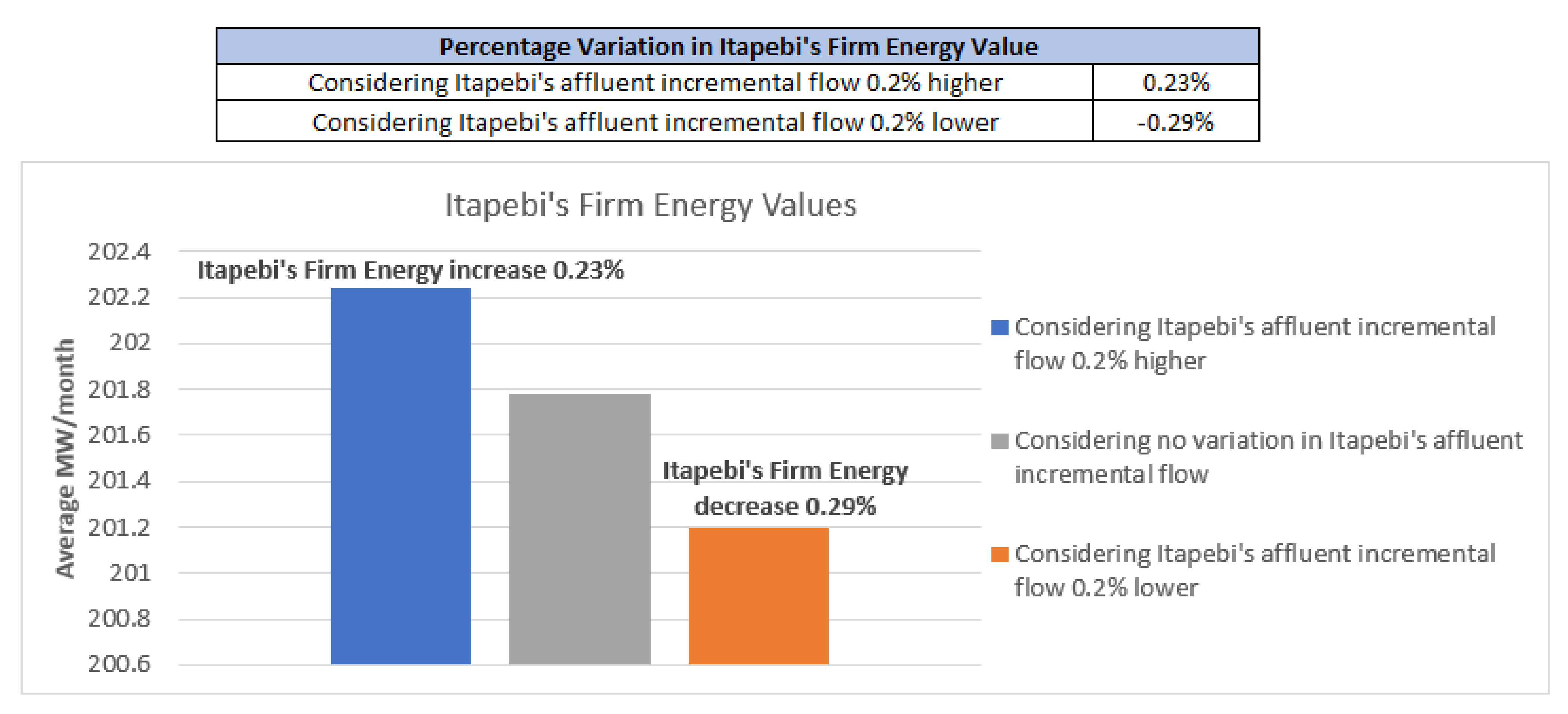
To evaluate the impact on the calculation of firm energy of a hydropower plant caused by a possible measurement error in the plant’s affluent incremental flow;
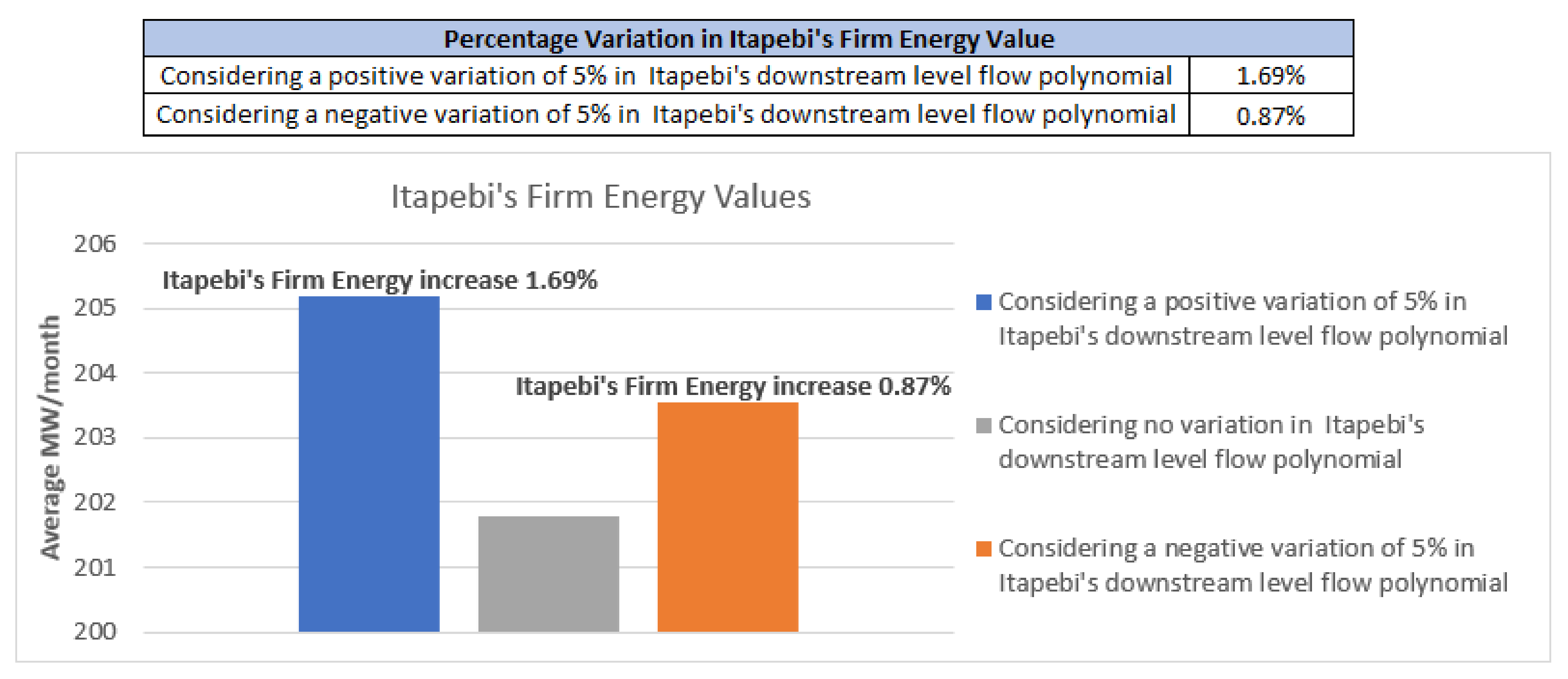
To evaluate the impact in the calculation of firm energy of a hydropower plant caused by a possible change in parameters of the plant’s downstream level flow polynomial.
As secondary contributions of this work, we can highlight:
Application of Dual Deterministic Dynamic Programming for the calculation of firm energy;
Application of the linear approach by parts of the hydroelectric generation in the calculation of firm energy;
Real case study in a large Brazilian hydropower plant.
2. Materials and Methods
The calculation of firm energy is a complex problem due to its size and the interconnection of cascading plants in the same hydrographic basin. This section presents the methodology used to model and solve this problem to calculate firm energy value from a plant in the Brazilian system.
As described in
Section 1.1, the firm energy of a hydropower plant corresponds to the maximum demand that can be met continuously in the event of recorded historical flows. In this section, a linear optimization model based on dynamic programming is presented to calculate the firm energy of the system and individualized hydropower plants as in [
21]. The mathematical formulation of the Linear Problem (LP) objective function and constraints of a given stage (t) is in
Section 2.2,
Section 2.3,
Section 2.4,
Section 2.5,
Section 2.6 and
Section 2.7. Each stage (t) is related to a time t with a corresponding LP. The input parameters of this subproblem are the so-called state variables, which for calculation, the firm energy are stored in the reservoirs at the beginning of the scenario and the deficit is found in the previous stage.
Due to the Brazilian system size and the study in terms of the operation problem, the linear optimization model presented does not include all of the system’s hydropower pants operational restrictions. Also, because of the elevated computational effort to solve this problem as a single linear problem, dynamic programming was chosen. Therefore, Dual Deterministic Dynamic Programming (DDDP) will be used to solve the problem. The description of DDDP is in
Section 2.1.
All performed simulations considered a full configuration of hydropower plants in the Brazilian power system. All necessary data are available from Monthly Energy Operation Program (PMO) of January 2021 [
20]. Monthly, the National System Operator (ONS)—the Brazilian Independent System Operator (ISO)—prepares and publishes the PMO with collaboration of all agents of the Brazilian power system. After that, the ONS provides all operation dispatch for the hydropower plants. To demonstrate hydropower’s firm energy behaviour, we will discuss the impact on the hydropower plant, as shown in
Section 1.2. It is essential to mention that all simulations time horizon started in January 1938 and ended in December 2018 with month periodicity. Moreover, the incremental flows were considered equal to the flows recorded in this period by the PMO [
20]. All the results of these simulations are presented in
Section 3.
2.1. Dual Deterministic Dynamic Programming
Dual Deterministic Dynamic Programming (DDDP) uses Benders Decomposition, which consists of dividing the problem into several stages. Each stage depends on the subsequent stage and, it is not necessary to discretize the entire state space of the problem. Thus, information obtained in the current period goes on to later periods allowing influences and interferences between them. For the problem solved in this article, each stage represents a period of time of the simulation period.
The objective is to obtain a possible solution to each stage’s subproblem by iteration and to build a linear approximation corresponding to the future impact function linked to the state variables related to these solutions. As the iterative process evolves and several points are visited, the model of future impact functions is progressively constructed.
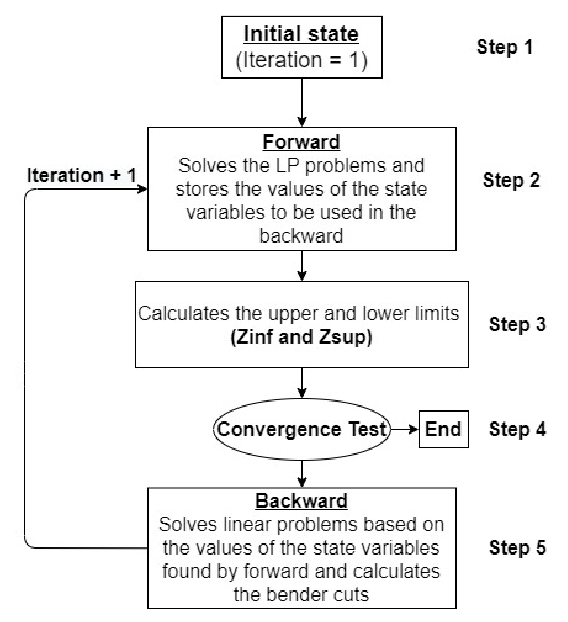
The solution through an iteration of DDDP is composed of two processes, forward and backward. The forward process starts at the first stage and ends at the last stage. In this process, there is a direct recursion which is solved through linear programming techniques without including information about the future impact.
In the backward process, the opposite path is followed. Starting at the last stage and ending at first. At each new stage, a constraint is generated for the future impact of the decision taken in the present concerning the previous stage, constructed through cuts from Benders (
1). This restriction will bring important information about the future impact of the decision taken at the present stage and, consequently, optmize the problem. The
Figure 3 shows the PDD flowchart.
where:
is the future impact of the decision taken in the present concerning the previous stage, constructed through cuts from Benders
is the Lagrange multiplier
is the derivative of the problem constraint, which has the state variable, in the state variable
is the value of the objective function found in stage t + 1
is the value found for the state variable in stage t for scenario u
In Step 3, presented in
Figure 3, the value of the lower limit (Zinf) and upper limit (Zsup) is calculated. The lower limit of the DDDP in an iteration k (
) is given by the optimal value found in the solution of the first stage of this iteration, Equation (
2). The Zsup of the forward solution
in an iteration
is given by Equation (
3).
Also, in
Figure 3, in Step 4, it is verified if the absolute difference between the upper and lower limits is less than a predetermined tolerance, Equation (
4). Therefore, this solution’s set is optimal and achieves algorithm convergence. Otherwise, the backward process begins, which will create a Benders cut for each previous recursive stage. Step 5 corresponds to the backward process, in which the restrictions for the following stages are formed based on the optimal solutions obtained by the forward process (Step 2).
where:
is the the tolerance limit adopted
is the number of a given iteration
is the upper limit of iteration k
is the lower limit of iteration iter
The next step is a new iteration, returning to the forward process in Step 2. However, now the Bender cuts created will be included. They will be restrictions on the problem. After this forward process has been finalized, a new optimal solution is found for the decision variables. Moreover, however, this iterative process continues.
As the iterative process evolves, the modelling of future impact functions is progressively improved by accumulating Bender cuts. Until the difference between the lower limit (Zinf) and the upper limit (Zsup) is equal to the tolerance adopted. This point corresponds to the convergence of the process. The next subsections present the modelling of each stage’s linear problems to be solved by the DDDP.
2.2. Objective Function
The objective function of each Linear Problem (LP) comprises the monthly energy deficit, the hydropower plant’s spillage, and an estimate of the future impact of the decision made. This estimate comes from the Benders cuts by solving the Dual Deterministic Dynamic Programming (DDDP) problem. Equation (
5) shows the complete objective function.
where:
is the number of hydropower plants in the system under study
t is the period of time
is the energy deficit value in period t
is the value of the slack variable in period t
is the penalty constant for the slack variable
is the constant penalty of spilled flow
is the spilled flow from plant j in time period t
is the estimated future impact for time period t + 1
In addition to the point above, the variable
decision variable accompanied by its penalty
must be inside the objective function. This variable, together with
, allows the problem to be decoupled into several subproblems. They must respect the constraint presented by Equation (
6).
is the energy deficit value in period t
is the energy deficit value in period t−1
is the value of the slack variable in period t
Since the variable
is highly penalized in the objective function, it is expected that its optimal value is equal to zero for all
t. As a result, the deficit for all stages will be equal to the deficit that occurred in the first month. Which does not have the restriction of Equation (
6). Since
is in the objective function, it will be minimized. In this way, the calculation of the firm energy of the system will be done as presented by Equation (
7).
where:
is the firm energy of the system
is the constant equal to the upper limit for firm energy. In this study, it was considered to be the sum of the installed powers of all hydropower plants in the system.
is the energy deficit value in period t = 1
With the optimal solution of the system’s firm energy defined, the values found for the system’s stored volume can be used to find the critical period. As described in
Section 1.1, it is the most prolonged time interval in which the reservoirs of the system’s set of plants start full and end empty without refilling. After defining this critical period, the firm energy of a hydropower plant can be calculated. It will be the average between the power generations of this plant during this period, as shown in Equation (
8).
where:
is the firm energy of hydropower plant j
is the hydroelectric generation of plant j during the critical period
is the number of stages of the critical period
2.3. Future Impact
The linear approximation by parts of the future impact estimate of the decision taken (Benders cut) of stage t is presented in Equation (
9). The Benders cut is formed by the set of (hyper) linear planes that provide a convex region of solution.
where:
is the number of hydropower plants in the system under study
t is the period of time
K is the set with all cuts
is the estimated future impact for time period t
is the coefficient of cut k that multiplies the stored volume of hydropower plant j, given by the Lagrange multiplier of the water balance equation of plant i in time period t + 1
is the coefficient of cut k that multiplies the energy deficit of period t + 1, given by the Lagrange multiplier of the equation to meet demand in time period t + 1
is the stored volume of plant j at the end of time period t
is the energy deficit value in the period at the end of the time period t + 1
is the independent coefficient of cut k at stage t+ 1
2.4. Energy Balance
Equation (
10) presents the restriction of meeting the system’s demand or energy balance. The sum between the hydroelectric energy generated and a possible energy deficit must be equal to the upper limit of the system’s firm energy, which will be considered to be the sum of the installed powers of all hydropower plants in the system.
where:
is the number of hydropower plants in the system under study
t is the period of time
is the hydroelectric generation of plant j in time period t
is the energy deficit value in period t
is the constant equal to the upper limit for firm energy. In this study, it was considered to be the sum of the installed powers of all hydropower plants in the system.
2.5. Water Balance
For each plant in the system, the plant volume stored at the end of stage t must be equal to the sum of its initial volume with the affluent incremental volume and the outflow volume of the upstream plants minus the outflow volume of the plant in question. The affluent incremental volume comes from the lateral volume between the plant and its upstream plants. In addition, the outflow volume is given by the sum between the turbined and spillage volumes. For the first stage,
t = 1, all stored volumes are considered equal to the plants’ maximum storage volume. In addition, the affluent incremental volume will be equal to the historical flows of the plant. The formulation of this water balance is presented in Equation (
11).
where:
J is the set of all hydropower plants in the system
C is the unit conversion constant, from m/s to hm , with a value of 2.592
is the stored volume of plant i at the end of time period t
is the stored volume of plant i at the beginning of time period t
is the affluent incremental flow of plant j in time period t
is the set of all hydropower plants upstream of plant j
is the flow turbined by plant m upstream of plant j in time period t
is the spilled flow by plant m upstream of plant j in time period t
is the flow turbined by plant j in time period t
is the spilled flow from plant j in time period t
2.6. Hydraulic Production Function
The generation of a hydropower plant is proportional to the difference between the upstream and downstream quotas. The upstream quota is given by a fourth-degree polynomial depending on the volume stored in the reservoir. The downstream quota is also given by a polynomial of the fourth degree, however, depending on the outflow of the plant (turbined flow plus spilled flow). In this context, study [
22] evaluates techniques of fitting a hydraulic turbine efficiency curve. In addition, studies in [
23,
24] evaluate techniques for predicting and prevent undesired spillage.
In the Brazilian system, the polynomials that define the upward and downward elevation were obtained in the past by adjusting a fourth-degree polynomial from values measured at each plant. For non-existing plants, these polynomials are estimated. Therefore, the hydroelectric generation of the plant can be calculated by a function that can be modelled by fourth-degree polynomials depending on the plant’s storage, turbination, and spilling.
However, with this representation, the optimization problem would become non-linear due to the introduction of the higher degree polynomial in the problem. As non-linear problems are more complex to be solved, Diniz and Maceira [
25] proposed an approximation of hydroelectric generation called the Approximate Hydraulic Production Function (AHPF). The objective is to perform a linear approximation by parts of the non-linear hydroelectric generation function, ensuring the convexity of the viable region defined by the function and maintaining the modeling of the problem as linear.
For the study, the linear approach by parts of the hydroelectric generation adopted was the strategy of discretizing the state space presented in [
26]. The discrete values of the volume stored in the reservoir, the turbine flow and the spilled flow are determined. In addition, the storage volume is discretized in
values between the maximum and minimum stored volume, the turbine flow in
values between the maximum and minimum turbine flow and the spilled flow in
values between zero and the maximum spilled flow. You get
discretized points and each n point (
) determines a value hydroelectric generation (
), given by Equation (
12).
With this, N points (
) are determined and from these points through a Convex Hull algorithm a convex surface bounded by the points is constructed. In the work [
27], the Qhull library [
28] that performs this procedure in an optimized way was used. Obtaining a set of P hyperplanes that represent the points discretized as a convex region. The Equation (
13) presents the restriction of hydroelectric generation.
where:
J is the set of all hydropower plants in the system
is the set of all hyperplanes obtained for plant j
is the stored volume of plant i at the end of time period t
is the flow turbined by plant j in time period t
is the flow spilled from plant j in time period t
is the constant parameter of hyperplane p for plant j
is the hyperplane parameter p associated with the stored volume of plant j
is the hyperplane parameter p associated with the turbine flow of plant j
is the parameter of the hyperplane p associated with the spilled flow of the plant j
Finally, a constant (
) is calculated to multiply the coefficients found for the AHPF. This constant is determined by minimizing the sum of the mean square error, as presented in [
25]. The objective is to reduce the error made by the convexification of the HPF. Thus, the final formulation used was that presented in Equation (
14).
2.7. Operating Limits of Variables
Finally, Equation (
15), Equation (
16), Equation (
17), Equation (
18), Equation (
19) and Equation (
20) show the operational limits of the problem variables.
where:
is the minimum storage volume of plant j
is the maximum storage volume of plant j
is the maximum flow that can be turbined by plant j
is the maximum flow that can be spilled by plant j
2.8. Applied Dual Deterministic Dynamic Programming
As presented in the previous sections, the calculation of firm energy can be formulated as an optimization problem represented by Equations (
5)–(
20). To solve this problem the technique of Dual Deterministic Dynamic Programming presented in
Section 2.1 is used. For a better understanding on how the iterative process of DDDP solves the optimization problem represented by Equations (
5)–(
20);
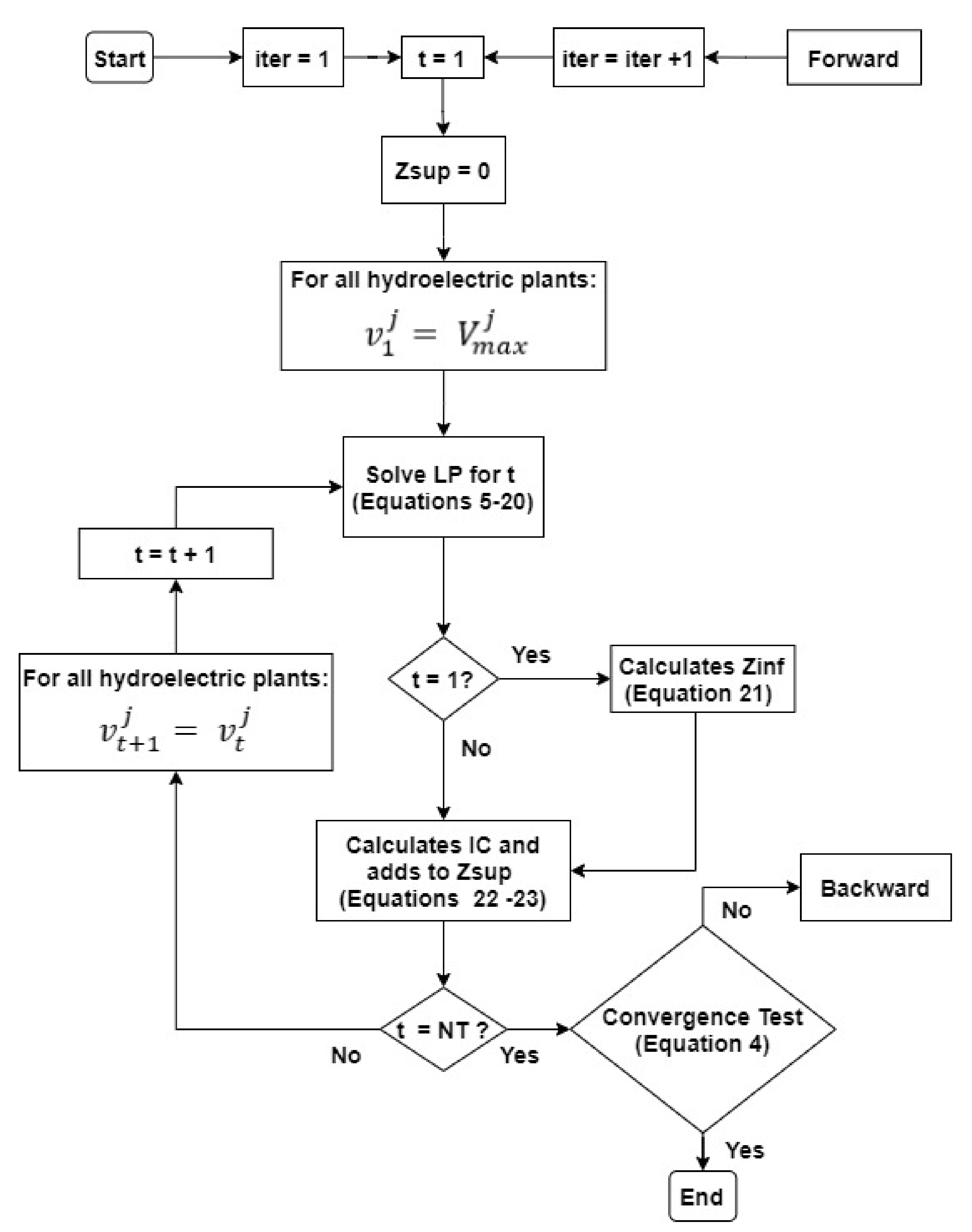
Figure 4 describes the forward process of DDDP.
When the algorithm starts the parameter that represents the number of iterations (
) is set equal to one. In the first stage (
), all the stored volume of the hydropower plants (
) is set equal to the maximum storage volume of the respective plant (
). After solving the first stage of the problem, the value of the lower limit
is calculated according to Equation (
21). For each stage after the first, the initial volume of each reservoir is equal to the final volume calculated in the previous stage. At the end of each stage, the variable
(upper limit) is increased by the value corresponding to the immediate cost, Equation (
22). Moreover, at the end of the forward process
will be equal to the sum of the immediate costs, Equation (
23).
where:
is the lower limit of iteration iter
is the immediate cost in period t of iteration iter
is the upper limit of iteration iter
is the total number of stages in the problem
is the number of hydropower plants in the system under study
t is the period of time
is the number of a given iteration
is the energy deficit value in period t
is the value of the slack variable in period t
is the penalty constant for the slack variable
is the constant penalty of spilled flow
is the spilled flow from plant j in time period t
is the estimated future impact for time period t + 1
After the last stage, if the absolute difference between
and
is less than a predetermined tolerance, Equation (
4), the algorithm converges and the iteration process ends. Otherwise, the backward algorithm in
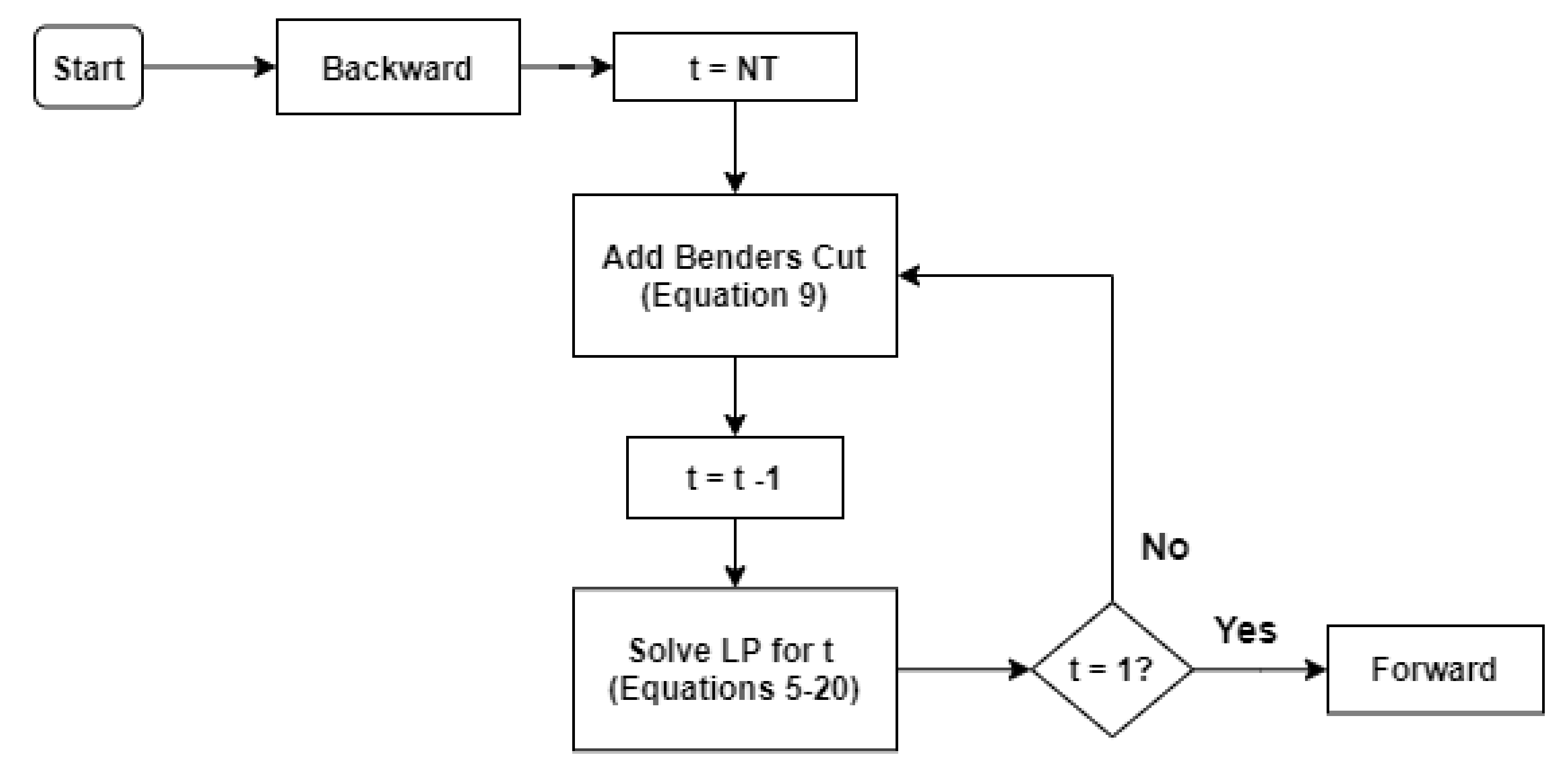
Figure 5 is invoked. At the end of the backward process, the forward process will be invoked again, starting a new iteration.
Figure 5 details the backward process, which is responsible for adding the restrictions given by Equation (
9) in the LP. It is noteworthy that at the beginning of the backward process the parameter that represents the time (
t) is equal to the last stage (
). Therefore, the coefficient
is given by the Lagrange multiplier of water balance equation of plant j (
11), and the coefficient
is given by the Lagrange multiplier of energy balance (
10). Finally, the independent coefficient
is given by Equation (
24).
where:
is the number of hydropower plants in the system under study
t is the period of time
is the coefficient of cut k that multiplies the stored volume of hydropower plant j
is the coefficient of cut k that multiplies the energy deficit of period t
is the stored volume of plant j at the end of time period t
is the energy deficit value in the period at the end of the time period t + 1
is the independent coefficient of cut k at stage t


 ,
, 


