
Optimal Pressure Management in Water Distribution Systems Using an Accurate Pressure Reducing Valve Model Based Complementarity Constraints


Abstract
1. Introduction
2. Existing Mathematical Model of PRV and the Newly Proposed PRV Model
2.1. Existing Model of Pressure Reducing Valves
2.2. An Accurate PRV Model Based Complementarity Constraints
3. Problem Formulation for Optimal Pressure Management
3.1. Objective Function
3.2. Constraints
3.2.1. The Continuity Equation at Node i
3.2.2. The Energy Equation for the Pipe Connecting Node i to Node j
3.2.3. Model Constraints for PRVs
3.2.4. Bound Constraints for Flows and Heads
3.2.5. The Reservoir Water Levels
4. Case Studies
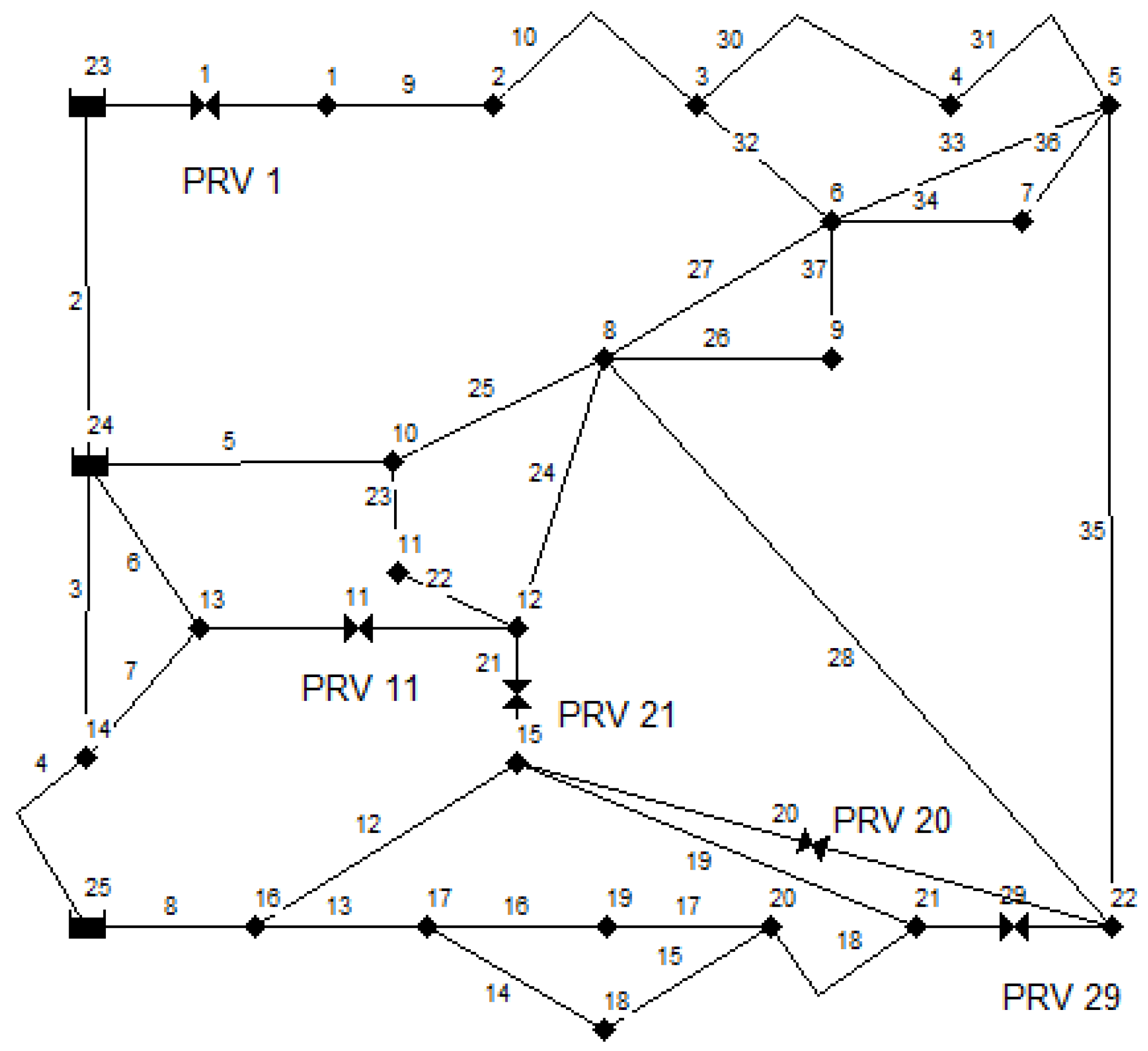
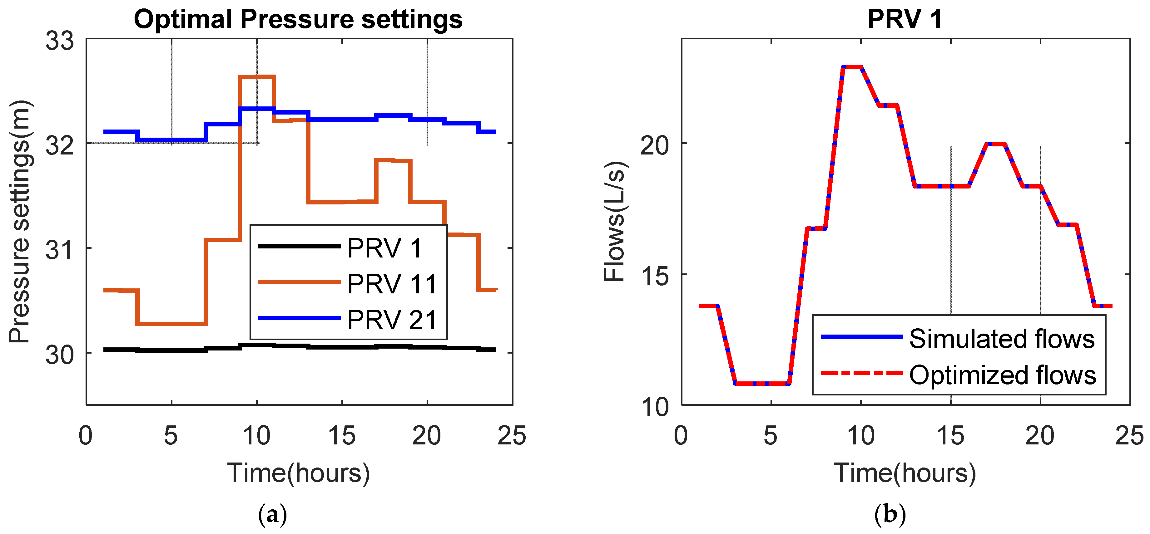
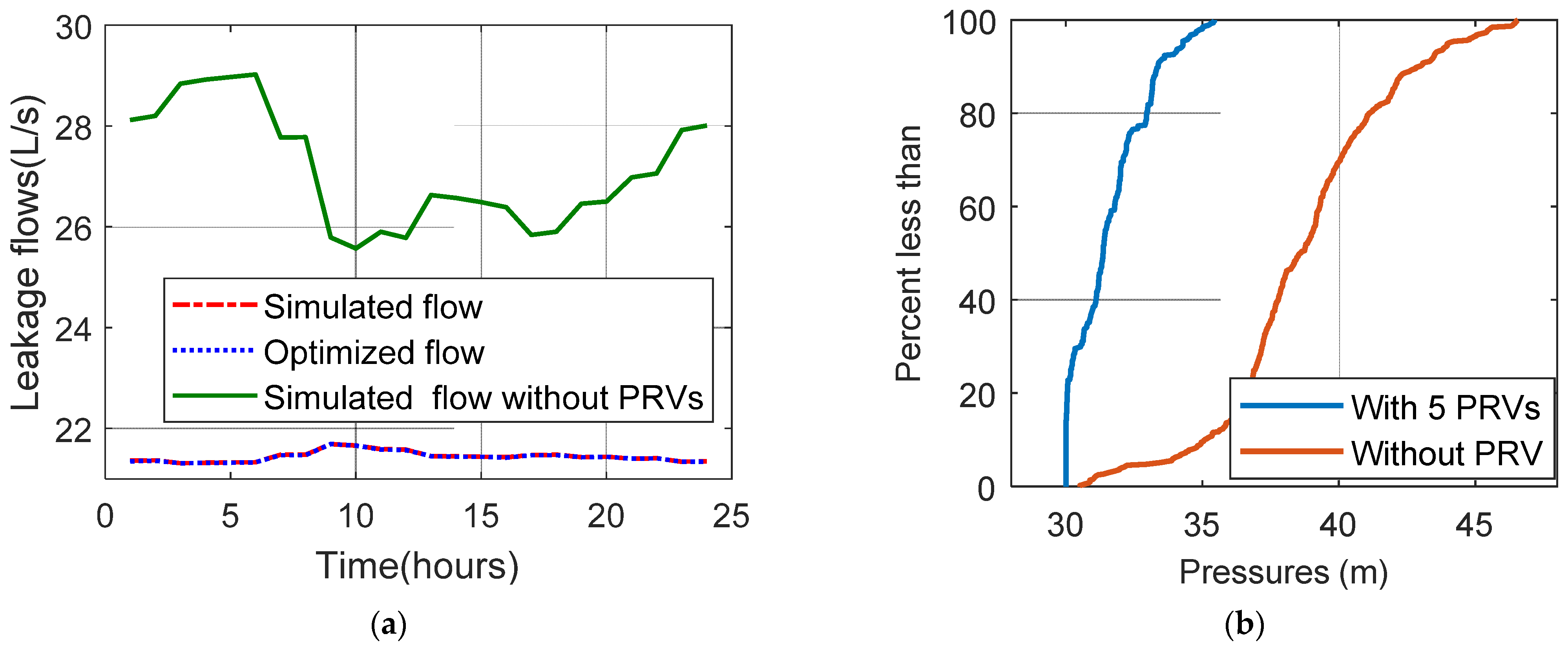
4.1. Case Study 1: Optimal Pressure Management for an Illustrative Water Distribution System with Multi Reservoirs
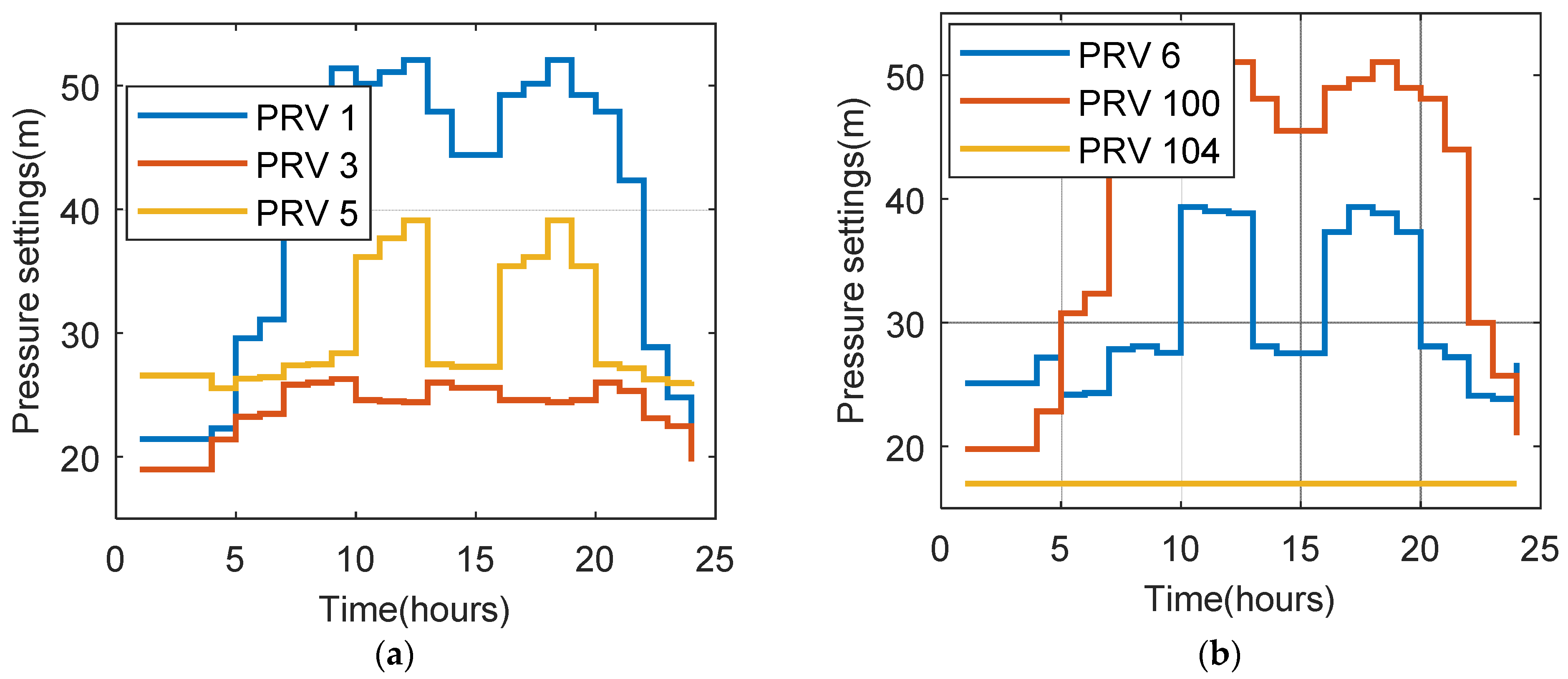
4.2. Optimal Pressure Management for a Benchmark Water Distribution System
4.3. Optimal Pressure Management for a Large Scale Water Distribution System in Vietnam
5. Conclusions
Supplementary Materials
Funding
Institutional Review Board Statement
Informed Consent Statement
Data Availability Statement
Conflicts of Interest
Nomenclature
| Hazen–William coefficient | |
| discharge coefficient of the orifice | |
| diameter and Hazen–William coefficient (m) | |
| demand at node i at time interval k (m3/s) | |
| nodal head at node i at time interval k (m) | |
| head loss across the link i, j at time interval k (m) | |
| index of time interval | |
| leakage at node i at time interval k (m3/s) | |
| length of link ij (m) | |
| static pressure at node i at time interval k (m) | |
| upper bounds of flows through links (m3/s) | |
| lower bounds of flows through links (m3/s) | |
| flow variables at time interval k (m3/s) | |
| leakage exponent | |
| variables in PRV model | |
| regularized parameter | |
| vector of variables for developing PRV model | |
| piecewise affine function (PWA) | |
| number of reservoirs | |
| number of links | |
| number of nodes |
References
- Giudicianni, C.; Herrera, M.; Nardo, A.D.; Adeyeye, K.; Ramos, H.M. Overview of Energy Management and Leakage Control Systems for Smart Water Grids and Digital Water. Modelling 2020, 1, 134–155. [Google Scholar] [CrossRef]
- Lambert, A.O. International report: Water losses management and techniques. Water Sci. Technol. Water Supply 2002, 2, 1–20. [Google Scholar] [CrossRef]
- Puust, R.; Kapelan, Z.; Savic, D.A.; Koppel, T. A review of methods for leakage management in pipe networks. Urban Water J. 2010, 7, 25–45. [Google Scholar] [CrossRef]
- Kouchi, D.H.; Esmaili, K.; Faridhosseini, A.; Sanaeinejad, S.H.; Khalili, D.; Abbaspour, K.C. Sensitivity of Calibrated Parameters and Water Resource Estimates on Different Objective Functions and Optimization Algorithms. Water 2017, 9, 384. [Google Scholar] [CrossRef]
- Taha, A.W.; Sharma, S.; Lupoja, R.; Fadhl, A.N.; Haidera, M.; Kennedy, M. Assessment of water losses in distribution networks: Methods, applications, uncertainties, and implications in intermittent supply. Resour. Conserv. Recycl. 2020, 152, 104515. [Google Scholar]
- Gupta, A.; Kulat, K.D. A selective literature review on leak management techniques for water distribution system. Water Resour. Manag. 2018, 32, 3247–3269. [Google Scholar] [CrossRef]
- Vicente, D.J.; Garrote, L.; Sánchez, R.; Santillán, D. Pressure management in water distribution systems: Current status, proposals, and future trends. J. Water Resour. Plan. Manag. 2016, 142, 04015061. [Google Scholar] [CrossRef]
- Araujo, L.S.; Ramos, H.; Coelho, S.T. Pressure control for leakage minimisation in water distribution systems management. Water Resour. Manag. 2006, 20, 133–149. [Google Scholar] [CrossRef]
- Mosetlhe, T.C.; Hamam, Y.; Du, S.; Monacelli, E.; Yusuff, A.A. Towards Model-Free Pressure Control in Water Distribution Networks. Water 2020, 12, 2697. [Google Scholar] [CrossRef]
- Dai, P.D.; Li, P. Optimal pressure regulation in water distribution systems based on an extended model for pressure reducing valves. Water Resour. Manag. 2016, 30, 1239–1254. [Google Scholar] [CrossRef]
- Skworcow, P.; Ulanicki, B.; AbdelMeguid, H.; Paluszczyszyn, D. Model predictive control for energy and leakage management in water distribution systems. In Proceedings of the UKACC International Conference on Control, Coventry, UK, 7–10 September 2010; pp. 1–6. [Google Scholar]
- Ulanicki, B.; Bounds, P.L.M.; Rance, J.P.; Reynolds, L. Open and closed loop pressure control for leakage reduction. Urban Water 2000, 2, 105–114. [Google Scholar] [CrossRef]
- Ulanicki, B.; AbdelMeguid, H.; Bounds, P.; Patel, R. Pressure control in district metering areas with boundary and internal pressure reducing valves. In Proceedings of the 10th International Water Distribution System Analysis Conference, WDSA2008. The Kruger National Park, Cape Town, South Africa, 17–20 August 2008; pp. 1–13. [Google Scholar]
- Prescott, S.L.; Ulanicki, B. Improved control of pressure reducing valves in water distribution networks. J. Hydraul. Eng. 2008, 134, 56–65. [Google Scholar] [CrossRef]
- Campisano, A.; Creaco, E.; Modica, C. RTC of valves for leakage reduction in water supply networks. J. Water Resour. Plan. Manag. 2010, 136, 138–141. [Google Scholar] [CrossRef]
- Creaco, E.; Franchini, M. A new algorithm for the real time pressure control in water distribution networks. Water Sci. Technol. Water Supply 2013, 13, 875–882. [Google Scholar] [CrossRef]
- Creaco, E. Exploring Numerically the Benefits of Water Discharge Prediction for the Remote RTC of WDNs. Water 2017, 9, 961. [Google Scholar] [CrossRef]
- Fontana, N.; Giugni, M.; Glielmo, L.; Marini, G.; Verrilli, F. Real-time control of a PRV in water distribution networks for pressure regulation: Theoretical framework and laboratory experiments. J. Water Resour. Plan. Manag. 2018, 144, 04017075. [Google Scholar] [CrossRef]
- Galuppini, G.; Creaco, E.; Toffanin, C.; Magni, L. Service pressure regulation in water distribution networks. Control Eng. Pract. 2019, 86, 70–84. [Google Scholar] [CrossRef]
- Galuppini, G.; Creaco, E.; Magni, L. A gain scheduling approach to improve pressure control in water distribution networks. Control Eng. Pract. 2020, 103, 104612. [Google Scholar] [CrossRef]
- Galuppini, G.; Magni, L.; Creaco, E. Stability and robustness of real-time pressure control in water distribution systems. J. Hydraul. Eng. 2020, 146, 04020023. [Google Scholar] [CrossRef]
- Burgschweiger, J.; Gnädig, B.; Steinbach, M.C. Optimization models for operative planning in drinking water networks. Optim. Eng. 2009, 10, 43–73. [Google Scholar] [CrossRef]
- Rossman, L.A. EPANET 2: User’s Manual; Rep. EPA/600/R-00/057; U.S. Environmental Protection Agency: Cincinnati, OH, USA, 2000.
- Savic, D.A.; Walters, G.A. An evolution program for optimal pressure regulation in water distribution networks. Eng. Optim. 1995, 24, 197–219. [Google Scholar] [CrossRef]
- Awad, H.; Kapelan, Z.; Savic, D. Optimal setting of time-modulated pressure reducing valves in water distribution networks using genetic algorithms. Integr. Water Syst. 2009, 13, 31–37. [Google Scholar]
- AbdelMeguid, H.; Ulanicki, B. Pressure and leakage management in water distribution systems via flow modulation PRVs. In Water Distribution Systems Analysis 2010; ASCE: Reston, VA, USA, 2021; pp. 1124–1139. [Google Scholar]
- Nicolini, M.; Zovatto, L. Optimal location and control of pressure reducing valves in water networks. J. Water Resour. Plan. Manag. 2009, 135, 178–187. [Google Scholar] [CrossRef]
- Liberatore, S.; Sechi, G.M. Location and calibration of valves in water distribution networks using a scatter-search meta-heuristic approach. Water Resour. Manag. 2009, 23, 1479–1495. [Google Scholar] [CrossRef]
- Creaco, E.; Pezzinga, G. Multiobjective optimization of pipe replacements and control valve installations for leakage attenuation in water distribution networks. J. Water Resour. Plan. Manag. 2014, 141, 04014059. [Google Scholar] [CrossRef]
- De Paola, F.; Giugni, M.; Portolano, D. Pressure management through optimal location and setting of valves in water distribution networks using a music-inspired approach. Water Resour. Manag. 2017, 31, 1517–1533. [Google Scholar] [CrossRef]
- De Paola, F.; Galdiero, E.; Giugni, M. Location and setting of valves in water distribution networks using a harmony search approach. J. Water Resour. Plan. Manag. 2017, 143, 04017015. [Google Scholar] [CrossRef]
- Mehdi, D.; Asghar, A. Pressure management of large-scale water distribution network using optimal location and valve setting. Water Resour. Manag. 2019, 33, 4701–4713. [Google Scholar] [CrossRef]
- Cao, H.; Hopfgarten, S.; Ostfeld, A.; Salomons, E.; Li, P. Simultaneous Sensor Placement and Pressure Reducing Valve Localization for Pressure Control of Water Distribution Systems. Water 2019, 11, 1352. [Google Scholar] [CrossRef]
- Sterling, M.J.H.; Bargiela, A. Leakage reduction by optimised control of valves in water networks. Trans. Inst. Meas. Control 1984, 6, 293–298. [Google Scholar] [CrossRef]
- Germanopoulos, G.; Jowitt, P. Leakage reduction by excessive pressure minimisation in a water supply system. Proc. Inst. Civ. Eng. 1989, 2, 195–214. [Google Scholar]
- Hindi, K.S.; Hamam, Y.M. Pressure control for leakage minimization in water supply networks: Part 2. Multi-period models. Int. J. Syst. Sci. 1991, 22, 1587–1598. [Google Scholar] [CrossRef]
- Vairavamoorthy, K.; Lumbers, J. Leakage reduction in water distribution systems: Optimal valve control. J. Hydraul. Eng. 1998, 124, 1146–1154. [Google Scholar] [CrossRef]
- Wright, R.; Stoianov, I.; Parpas, P.; Henderson, K.; King, J. Adaptive water distribution networks with dynamically reconfigurable topology. J. Hydroinform. 2014, 16, 1280–1301. [Google Scholar] [CrossRef]
- Ghaddar, B.; Claeys, M.; Mevissen, M.; Eck, B.J. Polynomial optimization for water networks: Global solutions for the valve setting problem. Eur. J. Oper. Res. 2017, 261, 450–459. [Google Scholar] [CrossRef]
- Gopal, V.; Biegler, L.T. Smoothing methods for complementarity problems in process engineering. AIChE J. 1999, 45, 1535–1547. [Google Scholar] [CrossRef]
- Hempel, A.B.; Goulart, P.J.; Lygeros, J. Strong stationarity conditions for optimal control of hybrid systems. IEEE Trans. Autom. Control 2017, 62, 4512–4526. [Google Scholar] [CrossRef]
- Hante, F.M.; Schmidt, M. Complementarity-based nonlinear programming techniques for optimal mixing in gas networks. EURO J. Comput. Optim. 2019, 7, 299–323. [Google Scholar] [CrossRef]
- Wächter, A.; Biegler, L.T. On the implementation of an interior-point filter line-search algorithm for large-scale nonlinear programming. Math. Program. 2006, 106, 25–57. [Google Scholar] [CrossRef]
- Drud, A.S. CONOPT—A large-scale GRG code. ORSA J. Comput. 1994, 6, 207–216. [Google Scholar] [CrossRef]
- Brook, A.; Kendrick, D.; Meeraus, A. GAMS, a user’s guide. ACM Signum Newsl. 1988, 23, 10–11. [Google Scholar] [CrossRef]
- Nguyen, K.D.; Duc Dai, P.; Quoc Vu, D.; Cuong, B.M.; Tuyen, V.P.; Li, P. A MINLP Model for Optimal Localization of Pumps as Turbines in Water Distribution Systems Considering Power Generation Constraints. Water 2020, 12, 1979. [Google Scholar] [CrossRef]


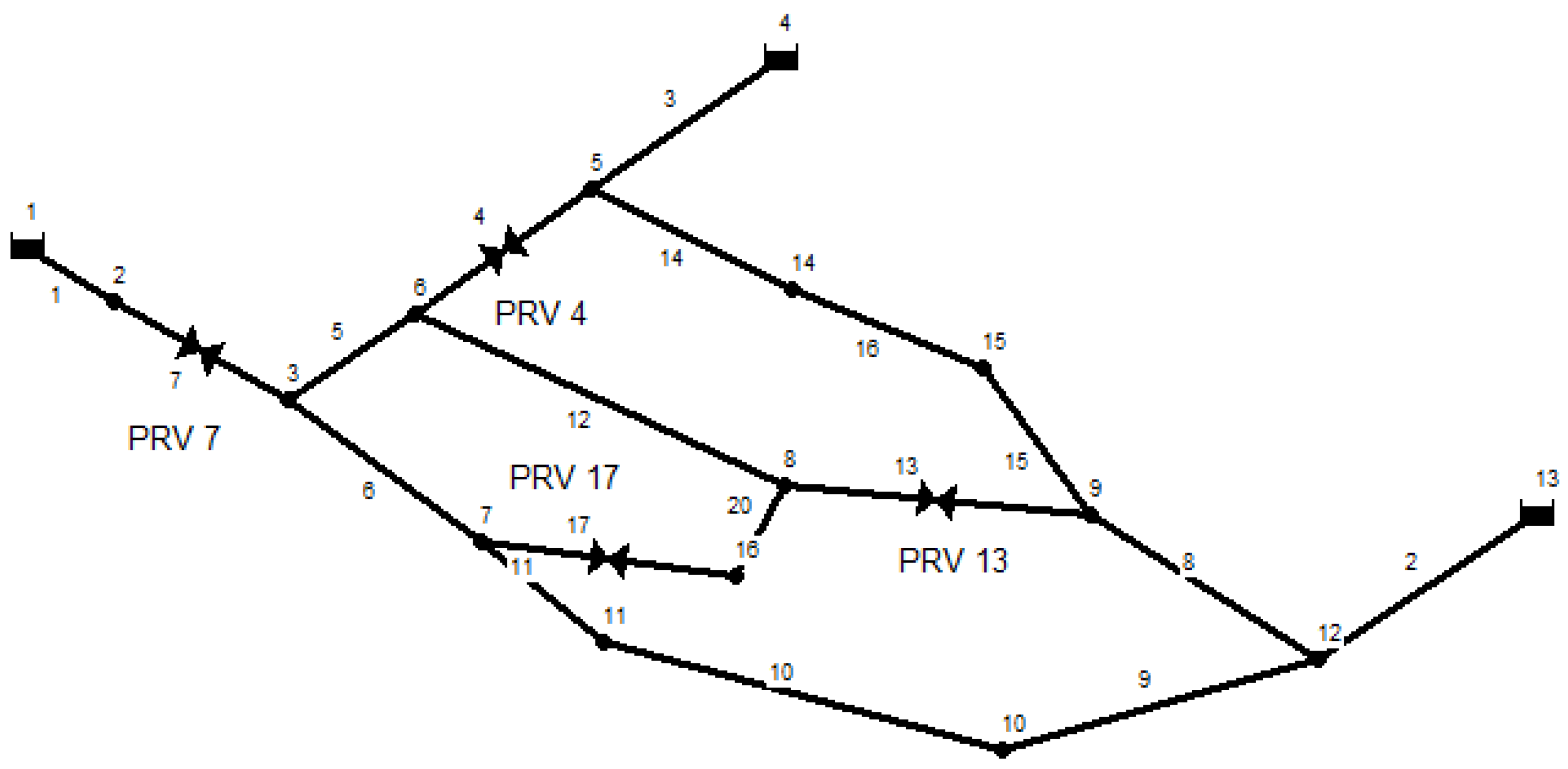
| Pipe ID | Start Node | End Node | Length (m) | Diameter (mm) | Node ID | Demand (L/s) |
|---|---|---|---|---|---|---|
| 1 | 1 | 2 | 100 | 300 | 2 | 100 |
| 2 | 13 | 12 | 100 | 350 | 3 | 0 |
| 3 | 4 | 5 | 150 | 200 | 5 | 0 |
| 4 | 5 | 6 | 500 | 200 | 6 | 300 |
| 5 | 6 | 3 | 0.01 | 200 | 7 | 300 |
| 6 | 3 | 7 | 200 | 300 | 8 | 100 |
| 7 | 2 | 3 | 150 | 300 | 9 | 50 |
| 8 | 12 | 9 | 100 | 300 | 10 | 50 |
| 9 | 12 | 10 | 200 | 300 | 11 | 30 |
| 10 | 10 | 11 | 100 | 300 | 12 | 50 |
| 11 | 11 | 7 | 50 | 300 | 14 | 20 |
| 12 | 6 | 8 | 300 | 400 | 15 | 10 |
| 13 | 9 | 8 | 150 | 300 | 1 | Source node with total head of 120.00 m |
| 14 | 14 | 5 | 50 | 300 | 4 | Source node with total head of 100.00 m |
| 15 | 15 | 9 | 50 | 300 | 13 | Source node with total head of 120.00 m |
| 16 | 14 | 15 | 500 | 300 | ||
| 17 | 16 | 7 | 250 | 300 |
| Time (Hours) | Demand Pattern | Time (Hours) | Demand Pattern |
|---|---|---|---|
| 1 | 0.61 | 13 | 0.92 |
| 2 | 0.61 | 14 | 0.92 |
| 3 | 0.41 | 15 | 0.92 |
| 4 | 0.41 | 16 | 0.92 |
| 5 | 0.41 | 17 | 1.03 |
| 6 | 0.41 | 18 | 1.03 |
| 7 | 0.81 | 19 | 0.92 |
| 8 | 0.81 | 20 | 0.920 |
| 9 | 1.23 | 21 | 0.82 |
| 10 | 1.23 | 22 | 0.82 |
| 11 | 1.13 | 23 | 0.61 |
| 12 | 1.13 | 24 | 0.61 |
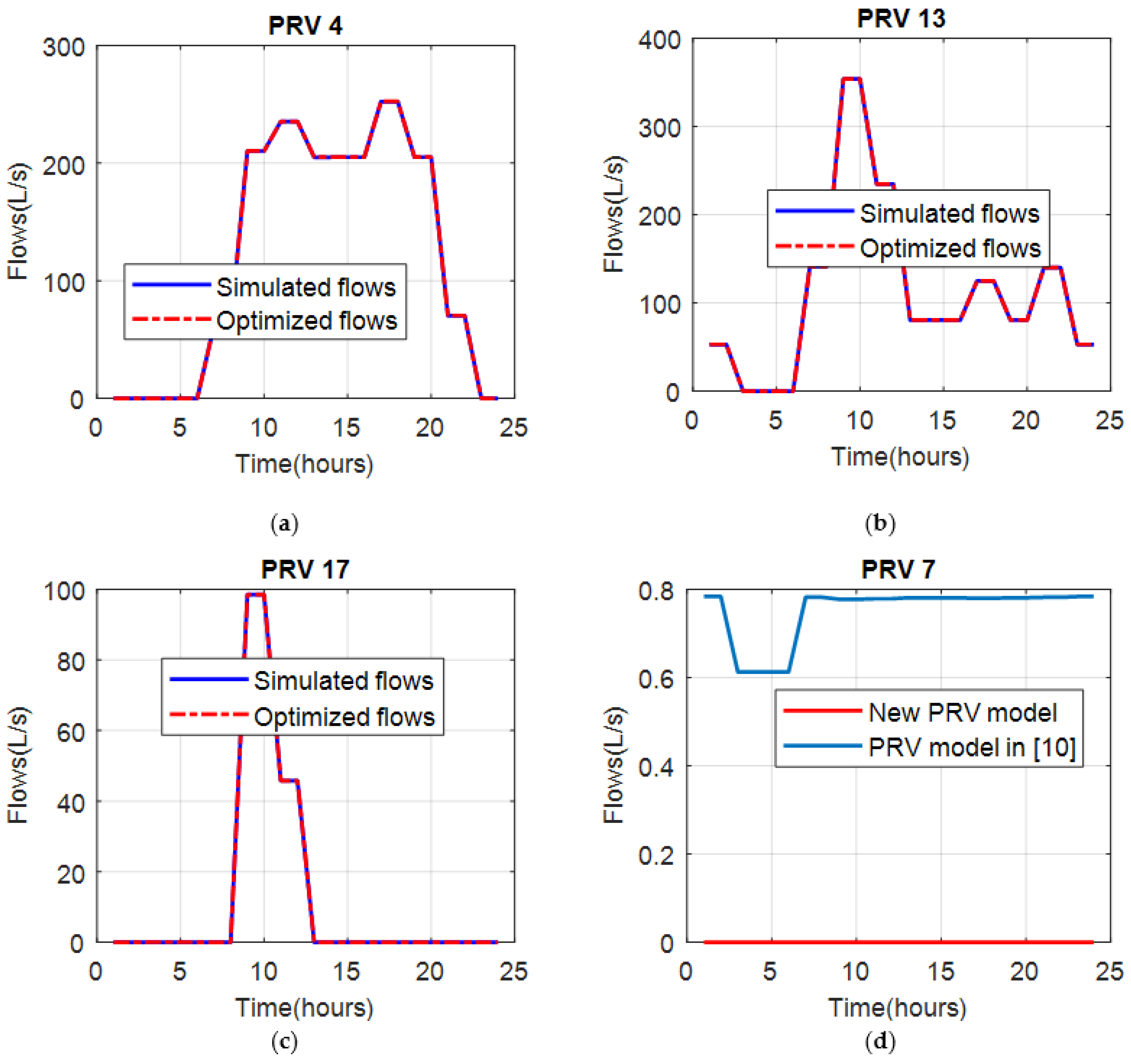
| Time (Hours) | PRV 4 | PRV 13 | PRV 17 | Time (Hours) | PRV 4 | PRV 13 | PRV 17 |
|---|---|---|---|---|---|---|---|
| 1 | Closed | 30.00 | Closed | 13 | 30.01 | 30.00 | Closed |
| 2 | Closed | 30.00 | Closed | 14 | 30.01 | 30.00 | Closed |
| 3 | Closed | Closed | Closed | 15 | 30.01 | 30.00 | Closed |
| 4 | Closed | Closed | Closed | 16 | 30.01 | 30.00 | Closed |
| 5 | Closed | Closed | Closed | 17 | 30.00 | 30.05 | Closed |
| 6 | Closed | Closed | Closed | 18 | 30.00 | 30.05 | Closed |
| 7 | 30.00 | 30.30 | Closed | 19 | 30.01 | 30.00 | Closed |
| 8 | 30.00 | 30.30 | Closed | 20 | 30.01 | 30.00 | Closed |
| 9 | 30.00 | 31.30 | 30.18 | 21 | 30.00 | 30.28 | Closed |
| 10 | 30.00 | 31.30 | 30.18 | 22 | 30.00 | 30.28 | Closed |
| 11 | 30.00 | 30.46 | 30.19 | 23 | Closed | 30.00 | Closed |
| 12 | 30.00 | 30.46 | 30.19 | 24 | Closed | 30.00 | Closed |
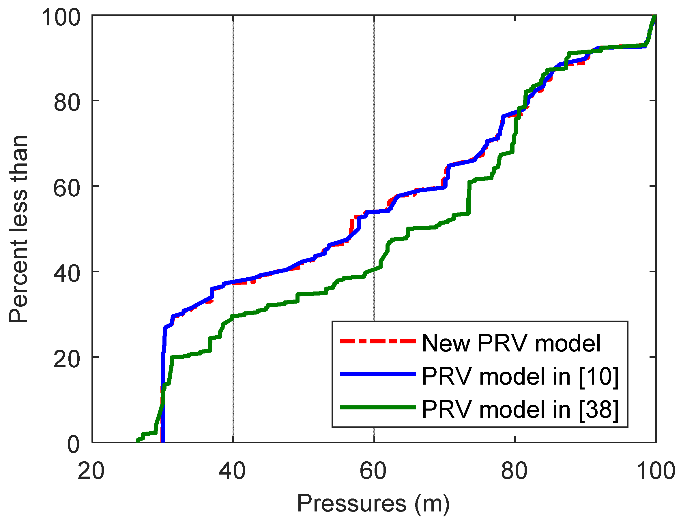
| PRV Model in [10] | PRV Model in [38] | PRV Model Based Complementarity Constraints | |
|---|---|---|---|
| Objective Function Values (m) | Objective Function Value (m) | Objective Function Value (m) | |
| 1 × 10⁻⁶ | 8731.49 | 10,118.95 * | 8694.83 |
| 1 × 10⁻⁷ | 8704.98 |
| PRV Model in [10] | PRV Model in [38] | PRV Model Based Complementarity Constraints | |
|---|---|---|---|
| Objective Function Values (m) | Objective Function Value (m) | Objective Function Value (m) | |
| 1 × 10⁻⁶ | 834.10 | 830.99 | 830.99 |
| 1 × 10⁻⁷ | 832.66 |
| Time (Hours) | Demand Pattern Factors | Time (Hours) | Demand Pattern Factors |
|---|---|---|---|
| 1 | 0.36 | 13 | 1.20 |
| 2 | 0.36 | 14 | 1.15 |
| 3 | 0.36 | 15 | 1.15 |
| 4 | 0.58 | 16 | 1.28 |
| 5 | 0.82 | 17 | 1.30 |
| 6 | 0.86 | 18 | 1.34 |
| 7 | 1.18 | 19 | 1.28 |
| 8 | 1.20 | 20 | 1.20 |
| 9 | 1.25 | 21 | 1.12 |
| 10 | 1.30 | 22 | 0.80 |
| 11 | 1.32 | 23 | 0.68 |
| 12 | 1.34 | 24 | 0.46 |
Publisher’s Note: MDPI stays neutral with regard to jurisdictional claims in published maps and institutional affiliations. |
© 2021 by the author. Licensee MDPI, Basel, Switzerland. This article is an open access article distributed under the terms and conditions of the Creative Commons Attribution (CC BY) license (http://creativecommons.org/licenses/by/4.0/).
Share and Cite
Dai, P.D. Optimal Pressure Management in Water Distribution Systems Using an Accurate Pressure Reducing Valve Model Based Complementarity Constraints. Water 2021, 13, 825. https://doi.org/10.3390/w13060825
Dai PD. Optimal Pressure Management in Water Distribution Systems Using an Accurate Pressure Reducing Valve Model Based Complementarity Constraints. Water. 2021; 13(6):825. https://doi.org/10.3390/w13060825
Chicago/Turabian StyleDai, Pham Duc. 2021. "Optimal Pressure Management in Water Distribution Systems Using an Accurate Pressure Reducing Valve Model Based Complementarity Constraints" Water 13, no. 6: 825. https://doi.org/10.3390/w13060825
APA StyleDai, P. D. (2021). Optimal Pressure Management in Water Distribution Systems Using an Accurate Pressure Reducing Valve Model Based Complementarity Constraints. Water, 13(6), 825. https://doi.org/10.3390/w13060825