The MATLAB HEC-RAS interface is tested first on an academical example, a rectangular canal, and then on a model of Beaver Creek to set up a control rule in the spirit of the work in [
22]. The first goal is to show that the automated start and stop simulations performed thanks to the designed interface lead to the same results as a manual simulation without restart. The second objective is that of defining closed-loop control rules for gates using the automated start and stop simulation to validate the approach. Moreover, the one-step simulations are performed by assuming that all hydrographs and control operations of gates are known beforehand for the whole simulation. Furthermore, note that no sudden modification of the input/output flows occurs during the one-step simulations. Likewise, the gate opening values do not change abruptly between two consecutive sampling instants. Indeed, HEC-RAS performs linear interpolation between the two values. Consequently, the resulting control strategies are faithful to reality, and are implemented in the custom user scripts.
4.1. First Case Study: The Rectangular Canal
The considered canal is 20,000 m long, with a width of 20 m and a normal depth of 9 m, while Manning’s roughness coefficient is equal to 0.04 for the whole canal. A cross section XS is considered every 10 m, except for the last one, and the geometry of all cross sections are exactly the same. This information is summarized in
Figure 4. There is one measurement station located at XS 700. Moreover, it is possible to simulate an offtake flow at XS 500. The input flow of the canal is controlled upstream, at XS 1000.
The evolution of the system is simulated for ten hours, with a control sampling time of one hour. The rationale behind this choice is motivated by the fact that the available data were sampled every thirty minutes, with some missing data. Therefore, re-sampling these data every hour allows to bypass this issue and fill in the missing data with average values. Nevertheless, the interface allows to consider the desired sampling time. Moreover, and while MATLAB scripts are executed every hour, the computation interval in HEC-RAS is equal to ten minutes. This means that the HEC-RAS process is executed six times per one MATLAB execution.
The initial condition considered downstream, i.e., XS 0, is given in
Table 3 as a stage hydrograph. The simulated upstream hydrographs, i.e., XS 1000, are defined according to two scenarios. The first one, labeled as
scenario1, is defined based on the pattern given in
Table 3. At the initial time, the upstream flow is equal to zero during ten minutes, then it is equal to 10 m
3/s for the next ten minutes, and so on. The second scenario, labeled as
scenario2, corresponds to a constant upstream inflow of 25 m
3/s, which can only cause the water level to increase. To mitigate this, the offtake flow located at XS 500 is controlled to withdraw water from the canal, thus avoiding overflow. The control rule described by Algorithm 1 consists in withdrawing water from the canal when the WSE at XS 700 exceeds 9.3 m. Note that a negative flow implies that HEC-RAS diminishes the canal flow, following the sign convention in [
22].
| Algorithm 1 Control rule for the rectangular canal |
if WSE at XS 700 is higher than 9.3 then set next value of lateral inflow hydrograph at XS 500 equal to 1−100 m3/s else set next value of lateral inflow hydrograph at XS 500 equal to 0 end if
|
In this first case study, and for both scenarios, the user must define the settings.ini file as indicated in Listing 2. Note that the starred values for XS 2, XS 3, and XS 4 denote interpolated cross sections.
 |
| Listing 2: Definition of settings.ini for the rectangular canal. |
Figure 5 shows the water level at XS 700 for
scenario1. The level increases and decreases according to the predefined upstream flow. The HEC-RAS results with automated start and stop simulations are depicted in dashed red, while the results without restart correspond to the continuous blue line. Note that the results obtained are identical for both methods, confirming that the MATLAB HEC-RAS interface approach performs as desired.
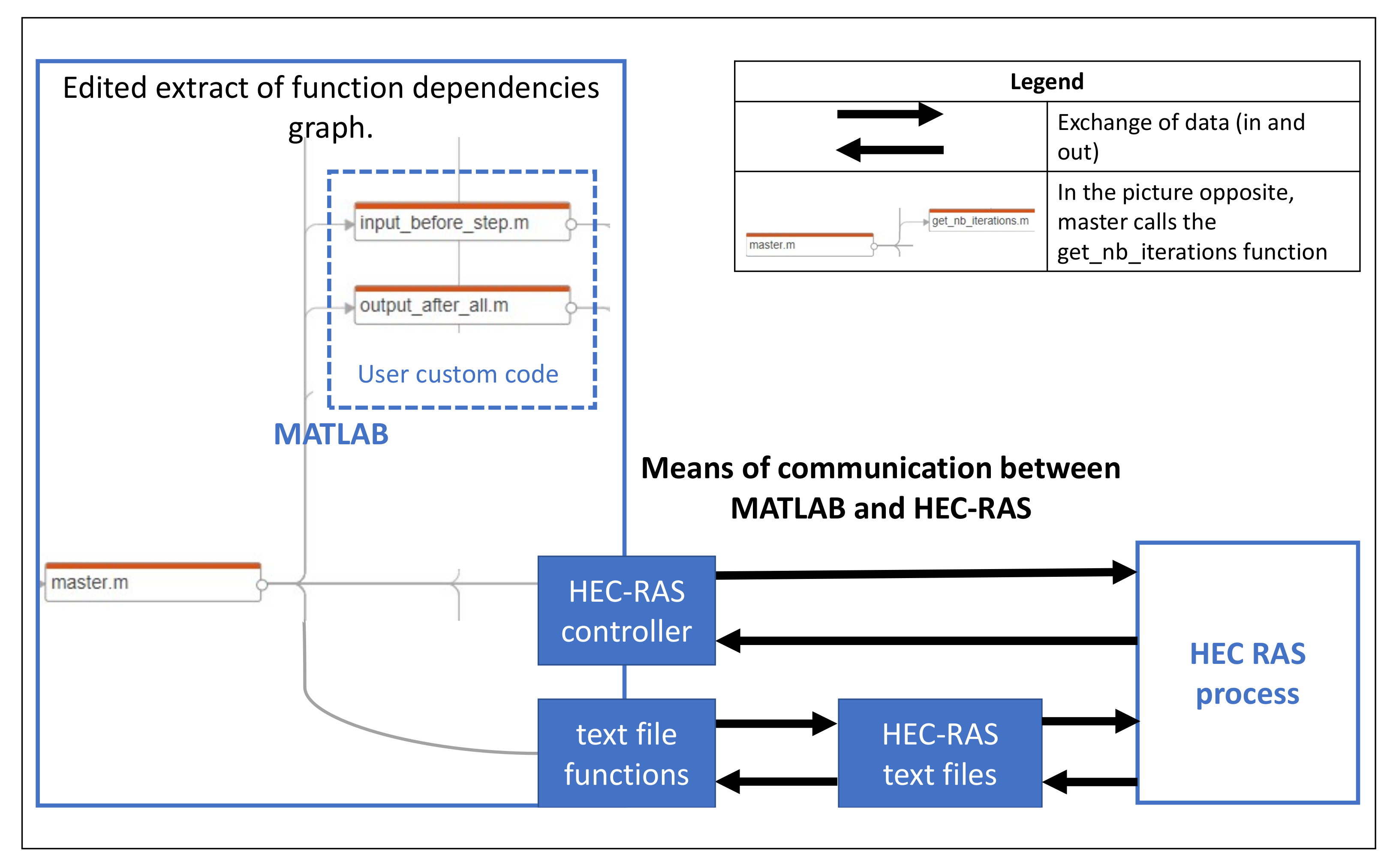
Regarding the second scenario, i.e., scenario2, the gate control rule is implemented in input_before_step.m as shown in Listing 3. This script is executed every hour, in accordance with the defined sampling time. Note that the variable ws_elev is assigned the current WSE (read from HEC-RAS), and xs{3} corresponds to an offtake flow, which is applied at the next steps of HEC-RAS.
On the other hand, Listing 4 shows how to access the WSE information from HEC-RAS using output_after_step.m.
 |
| Listing 3: Definition of input_before_step.m for the rectangular canal. |
 |
| Listing 4: Definition of output_after_step.m the for rectangular canal. |
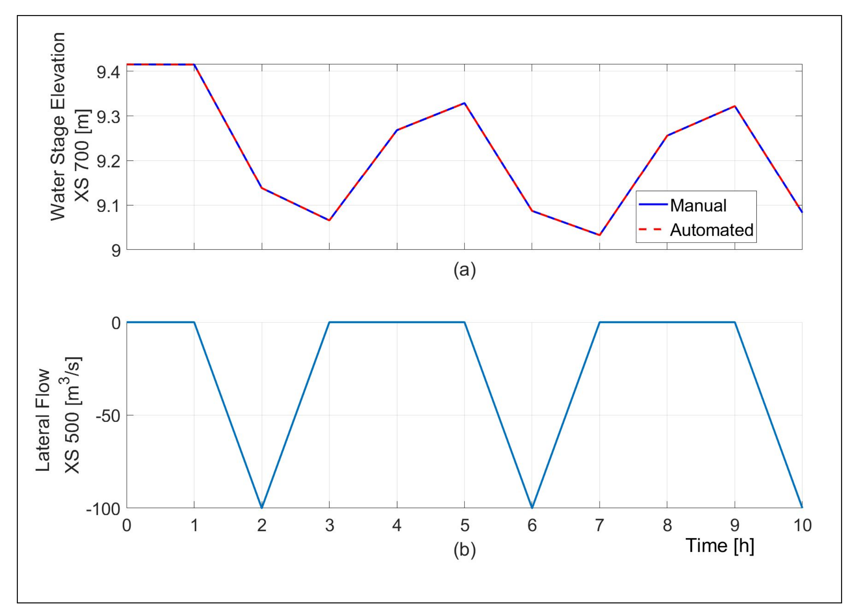
Figure 6a depicts the level at XS 700 for
scenario2, when the control rule is implemented. This rule requires to withdraw water from the canal whenever the level exceeds a height of 9.3 m. The lateral inflow hydrograph applied by the control rule to the offtake gate at XS 500 is presented in
Figure 6b. Note again that both approaches yield the same results. Thus,
scenario2 demonstrates the effectiveness of the control approach defined in MATLAB and its application in HEC-RAS thanks to the interface.
The most interesting feature of the first case study is that it allows to demonstrate the coordination possibilities between MATLAB and HEC-RAS. Moreover, advanced control algorithms can be easily implemented instead of the simple control rules, which only requires replacing the latter with the algorithm of choice. Indeed, this first case study depicts the basic functioning of the interface. In contrast, the following case study is closer to a real scenario.
4.2. Second Case Study: Beaver Creek
The Beaver Creek case study was proposed in [
22] (p. 116), and is based on the Bridge Hydraulics project, available for download on HEC-RAS website [
21]. Further information on how to set up and run this case study can be found on the MATLAB HEC-RAS interface documentation ([
27], Tutorial 1: simple automation example), which provides a step-by-step explanation to build a simplified version of this project.
Figure 7 presents the Beaver Creek HEC-RAS model with the cross sections and the locations of the measurement stations and the two gates, i.e., XS 5.61 and XS 5.44. The offtake gate located at XS 5.61 is used to withdraw water from the canal. Conversely, the inflow gate located at XS 5.44 is used to supply the canal with water. The initial and boundary conditions are summarized in
Table 4, and consist of a constant stage downstream hydrograph at XS 5.0 and a modification over time of the upstream flow at XS 5.99. Initially, the upstream flow is equal to zero, then it increases to 50 m
3/s for the next period, and so on. The sampling time for the HEC-RAS project and MATLAB are equal to twelve hours and one day, respectively.
The user must define, in settings.ini, the control points XS1 and XS2 that correspond to the cross sections XS 5.61 and XS 5.44, respectively. This is shown in Listing 5.
A new scenario is defined for the Beaver Creek case study, i.e., scenario3, which modifies the upstream hydrograph and implements a control rule in MATLAB. The rule controls the two gates based on conditions on the WSE value at XS 5.61. When this value exceeds a height of 65 m, the offtake gate located also at XS 5.61 opens, withdrawing 100 m3/s. As soon as the WSE is lower than 65 m, this gate is closed. On the other hand, when the WSE is lower than 64.5 m, the inflow gate opens to supply the canal with 20 m3/s. These control rules are summarized in Algorithm 2. Moreover, the file input_before_step.m is used to implement Algorithm 2, as shown in Listing 6.
| Algorithm 2 Control rule for the Beaver Creek case study |
if WSE in XS 5.61 is higher than 65 m then set next value of lateral inflow hydrograph at XS 5.61 equal to −100 m3/s and XS 5.44 to zero else if WSE in XS 5.61 is lower than 64.5 m then set next value of lateral inflow hydrograph in XS 5.44 equal to 20 m3/s and XS 5.61 to zero else set next value of lateral inflow hydrograph at both XS 5.61 and XS 5.44 equal to zero end if
|
 |
| Listing 5: Definition of settings.ini for the Beaver Creek case study. |
 |
| Listing 6: Definition of input_before_step.m for the Beaver Creek case study. |
Then, the WSE values can be obtained from HEC-RAS by conveniently modifying the output_after_step.m file, as shown in Listing 7.
 |
| Listing 7: Definition of output_after_step.m for the Beaver Creek case study. |
Figure 8a shows the automated start and stop results in dashed red, and the results without restart using a continuous blue line. Moreover,
Figure 8b,c depicts the lateral inflow hydrographs applied at XS 5.61 (offtake gate) and XS 5.44 (inflow gate), respectively.
scenario3 shows that the upstream flow modification and the control of the several gates based on one or several measurements of WSE are enabled by the MATLAB HEC-RAS interface. This approach can be easily extended to deal with advanced control algorithms for more complex systems, benefiting from the multiple functionalities offered by MATLAB and HEC-RAS.


