Nonlinear Water Quality Response to Numerical Simulation of In Situ Phosphorus Control Approaches

Abstract

The nonlinear and heterogeneous responses of nutrients to eutrophication control measures are a major challenge for in situ treatment engineering design, especially for large water bodies. Tackling the problem calls for a full understanding of potential water quality responses to various treatment schemes, which cannot be fulfilled by empirical-based methods or small-scale tests. This paper presents a methodology for Phoslock application based on the idea of object-oriented intelligent engineering design (OOID), which includes numerical simulation to explore the features of responses to numerous assumed schemes. A large plateau lake in Southwestern China was employed as a case study to illustrate the characteristics of the water quality response and demonstrate the applicability of this new approach. It was shown by the simulation and scenario analysis that the water quality response to Phoslock application always reflected nonlinearity and spatiotemporal heterogeneity, and always varied with objects, boundary conditions, and engineering design parameters. It was also found that some design parameters, like release position, had a significant impact on efficiency. Thus, a remarkable improvement could be obtained by cost-effective analysis based on scenarios using combinations of design parameters.

1. Introduction

Water eutrophication is one of the most serious problems in global water resource management [1]. The United Nations Environment Programme (UNEP) has investigated the phenomenon of water eutrophication around the world. The results show that about 30–40% of lakes and reservoirs are affected by eutrophication [2]. In 2019, the Chinese Ministry of Ecology and Environment monitored the nutritional status of 110 important lakes or reservoirs in China. The results showed that the proportion of lakes or reservoirs in a mesotrophic state was 62.6%, which is an increase of 0.9% over the previous year, including 25 lightly eutrophicated and six moderately eutrophicated water bodies [3]. At present, the aim of eutrophic water treatment is to remove nitrogen, phosphorus, and algae [4,5,6]. Many technologies for eutrophication control have been developed recently, such as phosphorus recovery [7], algae flocculation [8,9], oxygen nanobubble technology [10], and so on. Generally, these measures can be categorized in terms of external nutrient source reduction or in-lake restoration [11,12,13,14,15]. A great many modelling tools have been used to develop reasonable and effective schemes of external nutrient source reduction, such as Total Maximum Daily Loads (TMDLs) [16,17]. However, the same approaches are seldom applied to design in-lake measures, except for a few cases [15,18,19]. Most of those technologies designed with the intention of removing endogenous pollutants are based on pilot-scale trials or experience [20,21,22,23].

One of the endogenous control technologies, which is called phosphate binding, removes excess phosphate from water by adsorbing and inactivating phosphate and forming a new inert mineral called rhabdophane. The new mineral becomes part of natural lake sediments. Phoslock, which is the phosphate binder studied in this paper, was developed by the Commonwealth Scientific and Industrial Research Organization (CSIRO) in Australia in the 1990s and is made from lanthanum oxide and bentonite [24]. Phoslock has been widely used as a phosphorus adsorbent and an in situ sediment inactivation agent [25,26], but the size of receiving water bodies so far has been basically less than 2 km², according to the manufacturer’s website (www.phoslock.com.au, accessed on 16 February 2021). The application scheme for Phoslock is determined by pilot testing and experience [27,28], including position, frequency, and dose for spraying. It might be a reasonable approach for small-scale application, as the diffusion process often takes place relatively fast. However, each individual lake is an open complex system, and there are intricate nonlinear relationships between subsystems or various factors that make the response of nutrient concentration to treatment show nonlinearity and spatiotemporal heterogeneity [29,30]. For a large water body, like a lake with a surface area of several tens or even hundreds of square kilometers, empirical-based methods have difficulty dealing with such a complicated nonlinear system, and small-scale testing is not helpful. Therefore, a Phoslock application scheme determined by experience cannot achieve the expected effect for a large lake, and may result in huge waste. Apparently, from the perspective of cost-effectiveness, more precise and defensible methods are needed to guide the application of Phoslock for large projects.

The drawback of conventional engineering design for Phoslock application is a lack of quantitative analysis between numerous alternative schemes and potential outcomes. Thus, it cannot provide the information required by cost-effectiveness and non-compliance risk analysis, which are both concerns of decision-makers. This study presents a new methodology for Phoslock application based on the idea of object-oriented intelligent engineering design (OOID) [31], which might offer a possible solution to deal with the problem. Rather than overly relying on experience and assumptions, OOID focuses on predicting the water quality response for specific application modes through mechanistic models. In order to illustrate the methodology more clearly, this study explored the response of a large eutrophic lake to various scenarios of Phoslock application and analyzed the cost-effectiveness from different aspects. Based on the solid numerical simulation work, the methodology shown here could give a convincing argument when judging the pros and cons of scenarios or analyzing the doses required for different non-compliance risk levels caused by uncertainty. Due to the complexity and management implications of the OOID approach, it brings up a host of questions for research, and this study is only the beginning. All of the work and discussion in this paper do not aim to find an optimal scheme or develop a complete OOID process in practice, but are just an attempt to apply the idea to Phoslock projects in order to explore the nonlinear relationships between factors, generate insights, and provide a basis for future research.

2. Materials and Methods

2.1. Materials

Phoslock is a modified clay product that was developed to remove phosphorus from water bodies and eliminate the incidence of blue-green algal blooms. Phoslock, with its active ingredient lanthanum, is an emerging effective P-inactivation and blue-green algae management tool. The raw materials of Phoslock consist of an inactive clay-based carrier (bentonite), which comprises 95% of the product by weight, and the active ingredient lanthanum, which makes up 5% by weight. It is produced through an ion exchange process whereby lanthanum ions are exchanged with sodium ions from within the bentonite matrix. The lanthanum is bound to the surface of the clay, where it retains its ability to react with phosphate. Lanthanum is a strong binder of oxyanions such as phosphate. Binding with phosphate forms a mineral called rhabdophane (LaPO₄·nH₂O), which is highly insoluble and stable across a wide range of pH and redox conditions [24], such as those found in lake water and sediment. This property makes it ideal as a phosphorus binding agent, which can be put to use in lake restoration.

2.2. Methodology

2.2.1. Description of OOID

Instead of the inward perspective of traditional design approaches, OOID focuses on the objects to be protected, is concerned with the overall situation, accounts for the performance of single treating technology and its causal response relationship with environmental objects, and sets up multiple or single technologies at the right position, time, and scale in order to efficiently achieve the goal of environmental objects [31].

OOID makes judgments in advance based on relevant information, and then conducts in-depth analysis on the selection of various technologies, the collocation of position–scale–time, cost-effectiveness, optimal efficiency, and other issues, and produces various possible results. After that, the treatment scheme is finally determined, according to total cost, feasibility, and robustness. The OOID approach is more customizable and adaptable than conventional methods, and it gets away from arbitrary, disorganized, and abusive practices and some oversimplified assumptions and impractical hypotheses, which makes the effect more predictable and stable.

The OOID approach can be described step-by-step as follows [31].

• Compute the water quality response when applied to one single treating facility, expressed as the following equation.

  $$F\left(i\right)=f_i\left(X{1}_i,X{2}_i,X{3}_i\cdots ,X{n}_i\right)$$

  (1)

  where F denotes the quantification of response, derived from a set of parameters that characterize the facility and the circumstances, represented as $\left(X{1}_i,X{2}_i,X{3}_i\cdots ,X{n}_i\right)$. The functions are too complicated to express as analytical formulas, and researchers often compute them based on hydrodynamics and water quality modeling. Well-designed software is available. As such, the user does not need to code it from the beginning, but will likely have to modify the model in order to embed the treatment process within it.
• Compute the water quality response when applied to multiple facilities, expressed as the following equation:

  $$G\left(i\right)=g_i\left[m_i,f_i\left(X{1}_i,X{2}_i,X{3}_i\cdots ,X{n}_i\right)\right]$$

  (2)

  where G denotes the quantification of response and mi represents the scale factor. Due to the nonlinear process, when several facilities are deployed, and especially when they are located in different places, the comprehensive effect is not simply equal when adding it up. To obtain the answer, the model operations are still essential.
• Compute the water quality response when applied to multiple treatment technologies, expressed as the following equation:

  $$G\left(i\right)={\displaystyle \int }{g}_i\left[m_i,f_i\left(X{1}_i,X{2}_i,X{3}_i\cdots ,X{n}_i\right)\right].$$

  (3)

  Each technology and its object response, as well as the temporal and spatial optimization among various technologies, are not independent, but integrated into a causal system through intelligent design. ∫ represents the integration of all of those parameters at the object level. As discussed before, model computations are needed to analyze the comprehensive effect.
• Compute the object-oriented intelligent design.

  $$\left[m_i, X{1}_i,X{2}_i,X{3}_i\cdots ,X{n}_i\right]=\mathrm{lnv}G()$$

  (4)

  where InvG() denotes the reverse model of G. Based on the previous steps, the scale level and engineering design parameters that can achieve the goal of pollution control can be obtained by reverse computing.

2.2.2. Technical Framework of OOID-Phoslock

As discussed above, the OOID approach can generally be expressed from simple to complex in four steps. However, this study only focuses on developing the OOID approach on a Phoslock project (OOID-Phoslock). Therefore, computing the compounding effect of different technologies goes beyond the scope and step 3 is skipped. Steps 1 and 2 are merged in the modeling process, and, for cost-effective analysis, many scenarios as representative samples need to be created and simulated. Step 4 is mainly used to determine an operational plan constrained by the goal, which can be regarded as further work based on this study, but is not included here. The specific technical framework of OOID-Phoslock is shown in Figure 1.

Position, dose, application season, and frequency are the main variables in scenario generation, but they are not enough for a comprehensive evaluation. Since the lake is a highly dynamic system, its external boundaries, such as inflow and meteorological conditions, constantly vary and impact the hydrodynamic characteristics and water quality both directly and indirectly. These uncertainty factors may affect the response of water quality to Phoslock. Thus, these factors could make the simulated results deviate from the real situation, and the deviation would lead to inaccurate decisions and cause problems, such as failing, to meet the goals or use an excessive dosage. Therefore, it is necessary to take the boundary conditions as disturbance variables.

To assess the water quality response to Phoslock application, this study uses an entire watershed and lake modeling system. As shown in Figure 2, the system consists of six components, and can be classified into two main parts. One part is the watershed model (hydrological and pollutant loading model), and the rest is the lake model. The watershed model parameterizes the watershed and outputs time series, such as flow and pollutant flux, which are required by the lake model as boundary conditions. Packages like the Hydrologic Simulation Program–FORTRAN (HSPF) [32], Soil and Water Assessment Tool (SWAT) [33], Loading Simulation Program C (LSPC) [34], MIKE SHE (coupled with MIKE ECO-Lab) [35,36], or other similar software can simulate the watershed as required. The lake model simulates the behavior of contaminants in water, organisms, and sediment under boundary conditions. The data output feed all the analyses of this study. Software like EFDC [37], Delft 3D [38,39], MIKE3 (coupled with MIKE ECO-Lab) [36,40], and the like can produce simulations of the hydrodynamics and water quality in lakes. Since the study needed to simulate water quality when applying Phoslock, the action of Phoslock in the lake had to be expressed in the modelling system. However, no existing software has such a module. This part had to be created and embedded in the lake model. The required capability of models is shown in Figure 2 and the available competent software is listed in

Table 1. Models in the simulation system and available software.

Domain	Description	Output	Software Available
Basin	Distributed or semi-distributed hydrological model	Flow time series	HSPF, SWAT, LSPC, MIKE SHE+MIKE ECO-Lab, etc.
	Watershed-scale water quality and nonpoint source (NPS) pollution model	Pollutant flux time series
Lake	Hydrodynamic simulation	Water level and flow direction time series	EFDC, Delft 3D, MIKE3+MIKE ECO-Lab, etc.
	Heat exchange simulation	Water temperature time series
	Nutrient transport and transformation simulation	Water quality time series
	Endogenous dynamic simulation
	Simulate dissolution, binding (with phosphate), precipitation process of Phoslock in the lake		_

. The whole simulation system is continuous and dynamic, and can provide feedback on any change of boundary conditions.

2.3. Case Study

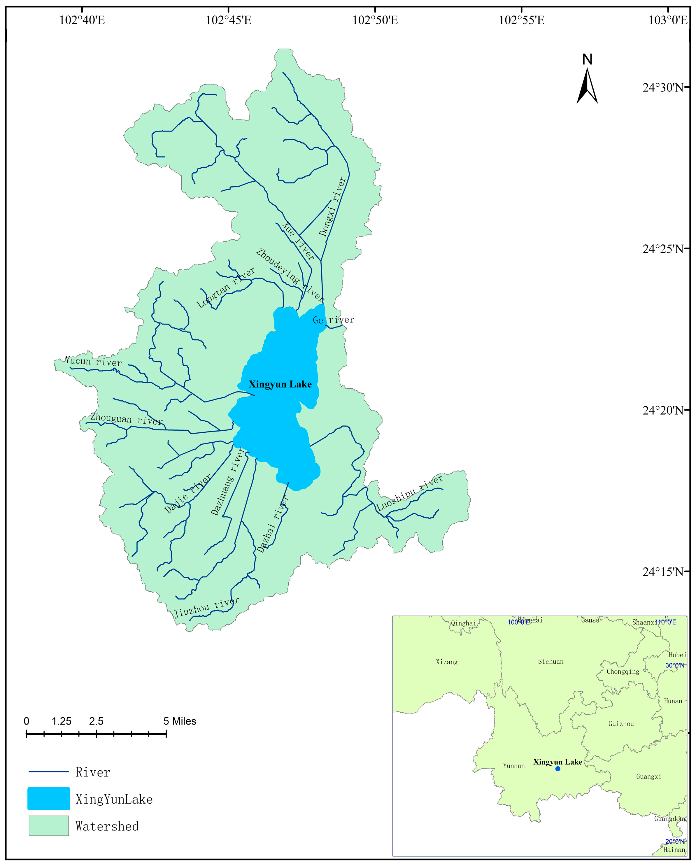
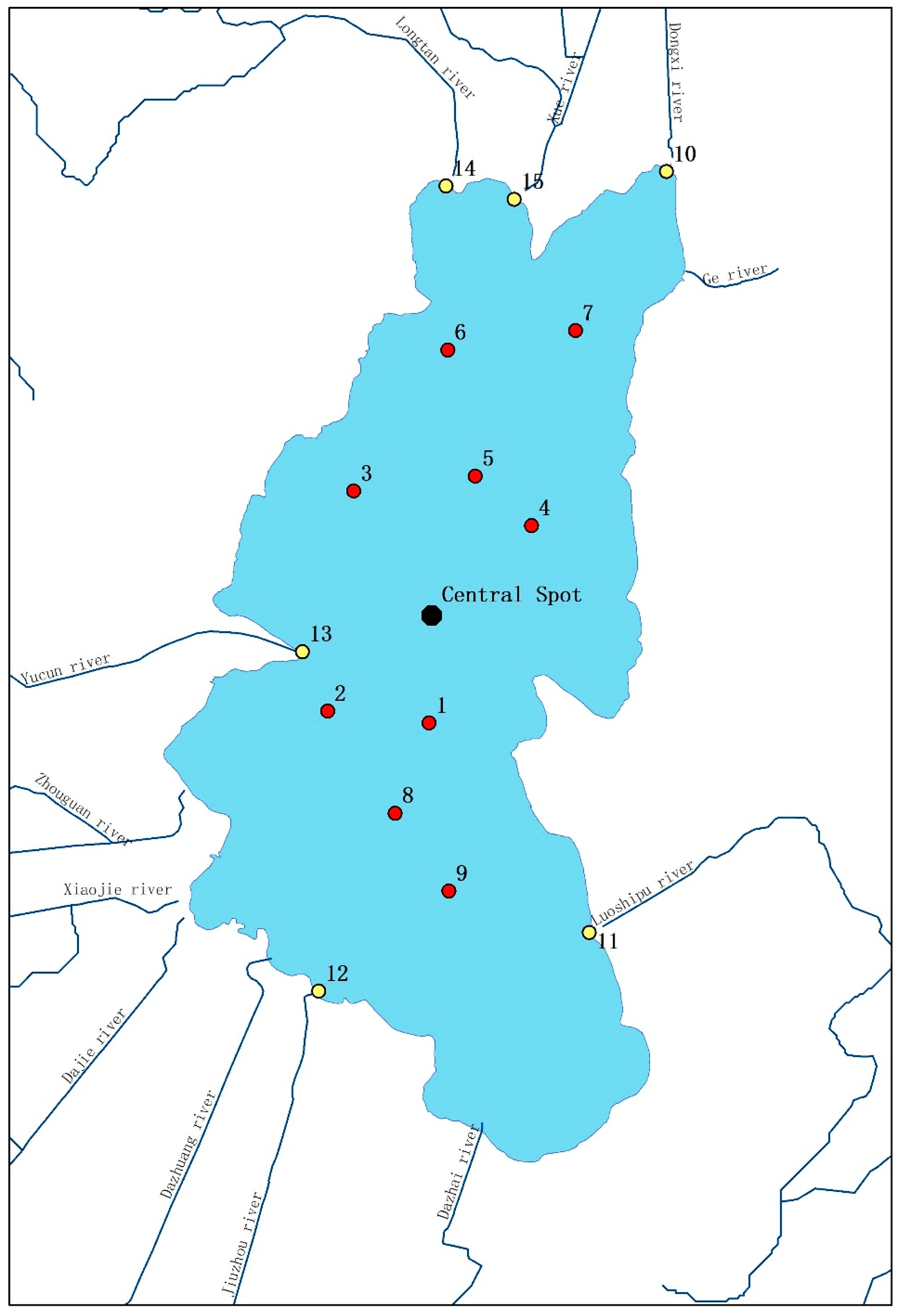
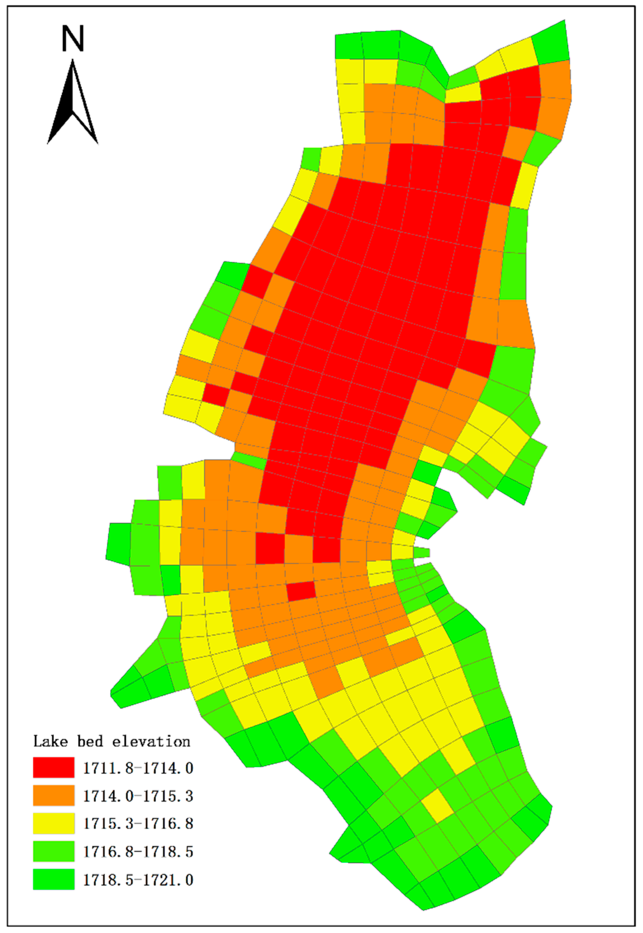
2.3.1. Study Area

Lake Xingyun is one of the nine largest plateau lakes in Yunnan Province, Southwestern China (Figure 3). It has a normal elevation of 1722 m [41], an average lake depth of 7 m, and a maximum depth of 10 m. The total area of the watershed is 358 km², and the lake surface area is 34.7 km² with a volume of 1.84 × 10⁸ m³ [42,43]. It is hydrologically recharged by precipitation and seasonal inflows from more than 12 small, intermittent rivers. The mean annual water inflow is about 6.2 × 10⁷ m³ [44].

Historical water quality data shows that the water quality of Xingyun Lake has been deteriorating since 1998. The lake met the standards set for drinking water sources (environmental quality standards for surface water, grades I–III) before 1998, and then met a lower standards (grade IV) set for general water use in industry and recreation or agriculture between 1999–2001. After that, the water was only suitable for agricultural use (grade V), the lowest level in Chinese water quality standards, and has even turned worse over recent years. From 2015 to 2017, according to the monitoring data, six conventional water quality indicators exceeded the limits of grade V, and the worst was total phosphorus (TP). In addition, Microcystis aeruginosa, a species of freshwater cyanobacteria that can form harmful algal blooms, has become the dominant species in the lake all year round, and the water ecosystem has been severely impaired by eutrophication and cyanobacteria blooms.

In order to reverse the degradation of the water quality and ecology of Xingyun Lake, the local government has made great efforts to reduce the pollutant flux discharged from the land surface into the lake. However, due to the serious pollution and high phosphorus level, improving the water quality significantly lags behind all these measures, which calls for the assistance of in situ remediation treatment of the lake, most urgently to get rid of the excess phosphorus and control the outbreak of cyanobacteria. Consequently, several projects aiming to remove or inactivate the endogenous pollutants in Xingyun Lake have been put on the agenda, including the release of Phoslock.

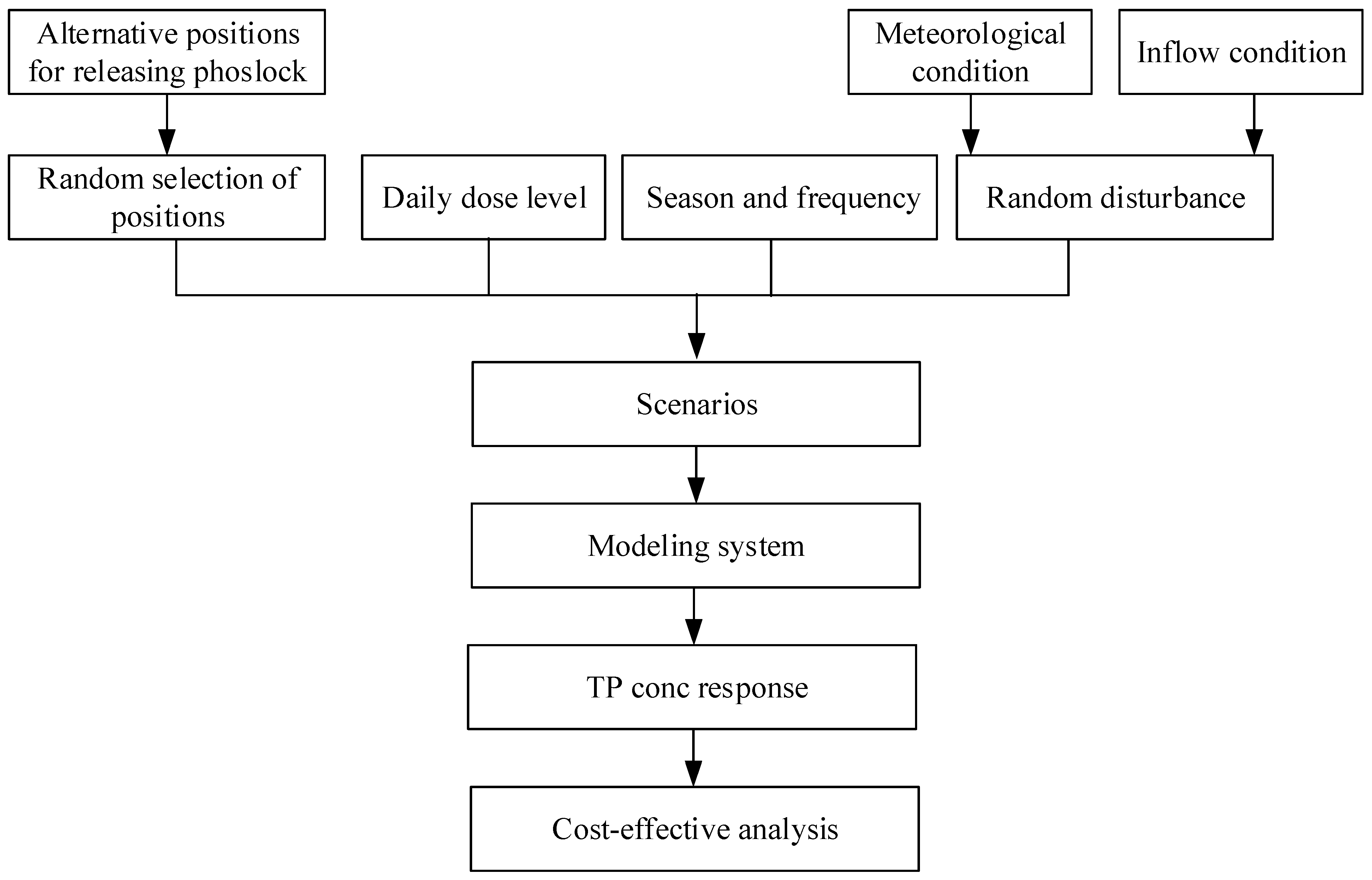
2.3.2. Scenario Generation

A total of 1944 scenarios were finally generated by the scenario generation program, according to the steps shown in Figure 1. The variables were position, dose, season, and uncertainty factors, but the frequency and applying mode were unchanged. All the positions in one scenario had an equal dose, in case too many scenarios were created. The simulation period was properly set based on the research. The combination of design parameters is shown in

Table 2. Permutations and combinations of design parameters.

Season	Sets of Positions	Number of Dose Ranks	Uncertainty Classification	Count
First (T1)	8 (artificial)	9 (10–300 t/d)	3 (base 0~base 2)	216
	10 (random)	9 (10–300 t/d)	3 (base 0~base 2)	270
Second (T2)	8 (artificial)	9 (10–300 t/d)	3 (base 0~base 2)	216
	10 (random)	9 (10–300 t/d)	3 (base 0~base 2)	270
Third (T3)	8 (artificial)	9 (10–300 t/d)	3 (base 0~base 2)	216
	10 (random)	9 (10–300 t/d)	3 (base 0~base 2)	270
Fourth (T4)	8 (artificial)	9 (10–300 t/d)	3 (base 0~base 2)	216
	10 (random)	9 (10–300 t/d)	3 (base 0~base 2)	270

, and the details are explained as follows.

● Position

Two positions for spraying Phoslock were considered: river estuaries and internal sites of the lake. Six estuarine sites and nine typical internal sites were assigned as the optional positions, so there were 15 positions available to select, and each scenario had five positions to release Phoslock. First, eight sets of positions were artificially selected for different seasons (discussed in the next section) in order to explore the temporal variability of the water quality response and the average response over seasons for the same positions. Second, for each season, 10 sets of positions were randomly selected from 15 places, and these 40 (4 × 10) sets of positions were expected to be different from each other. At the end, each season had 18 sets of positions, with eight of them identical for four seasons, and the other 10 sets were distinct. As shown in Table 2, there were 864 (216 × 4) scenarios with artificially selected positions and 1080 scenarios with randomly selected positions. All the positions were numbered, as shown in Figure 4, and the artificial sets are presented in

Table 3. Artificial sets of release positions.

Code Name	Position Numbers
A0	1, 2, 3, 4, 5
A1	1, 2, 3, 4, 13
A2	10, 11, 12, 14, 15
A3	1, 2, 5, 6, 7
A4	2, 3, 4, 5, 13
A5	1, 2, 10, 14, 15
A6	3, 4, 5, 11, 12
A7	1, 2, 10, 13, 15

.

● Dose and application mode

The daily dose was ranked in nine levels: 10, 20, 30, 40, 60, 90, 120, 180, and 300 tons per day (t/d). The application mode for all scenarios was identical, with five positions rotated to release Phoslock by day, and the operation was arranged daily from 09:00 to 17:00.

The Phoslock release period was set during each season and continued without interruption for 30 days in every period, and the start date of the periods was set on the 63rd day (T1), 142nd day (T2), 246th day (T3), and 342nd day (T4) in a year.

● Uncertainty factors

To make the results more reliable, based on sensitivity and uncertainty analysis of parameters, two types of adjustment coefficient of inflow, TP concentration, wind direction, and wind speed are set. One is a fixed coefficient to determine the overall change of each factor, and the other is a random disturbance coefficient to express the uncertainty of each factor in the time series. Three baseline scenarios (base0, base1, and base2) for uncertainty conditions are generated for each release.

● Simulation period

All scenarios produced following the above method were simulated by the modeling system (which will be covered in the next section) and output the response of TP concentration in Xingyun Lake for each scenario. Before the formal simulation, two scenarios with a release period of 30 days and a simulation period of 550 days, and two dosages of 10 and 300 t/d were simulated as an experiment to determine a reasonable simulation period. According to an analysis of the results, the cumulative value of TP concentration improvement accounted for more than 70% of the whole simulation period of 550 days when the simulation time was 200 days. To save time, the simulation period for all scenarios was set as 200 days.

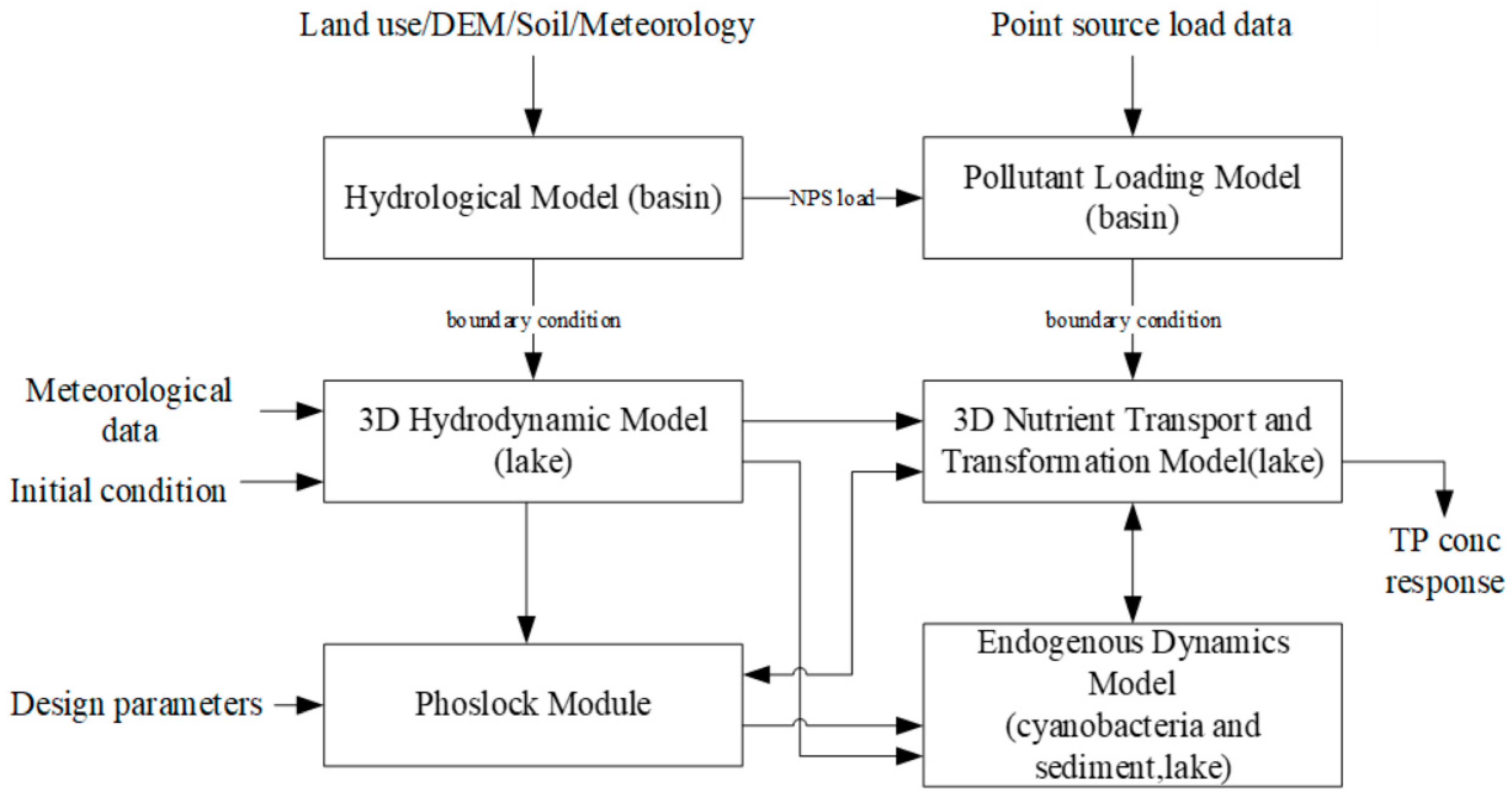
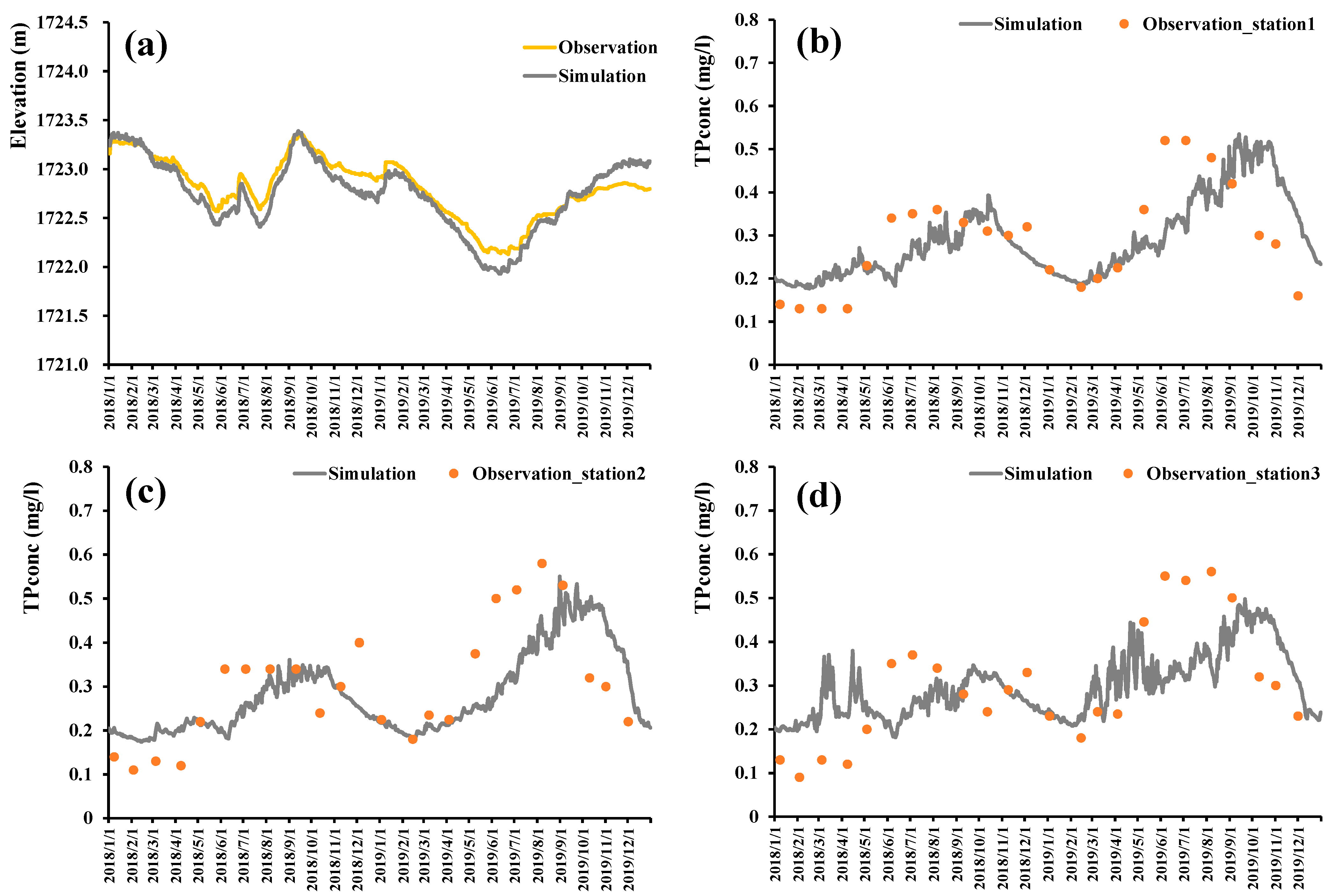
2.3.3. Modeling Process

In this case, LSPC and EFDC were adopted as the watershed and lake models, respectively. The hydrological and pollutant loading process in Xingyun Lake Basin from 1 January 2016 to 31 December 2019 was simulated by LSPC. Accordingly, the time series of streamflow and flux of nutrients that discharged into the lake were acquired and used to drive the EFDC model. The EFDC model and the Phoslock module simulated the hydrodynamics and water quality under the action of Phoslock. The principles of the EFDC model and the Phoslock module are introduced in Supplementary Materials. Below is a description of the Xingyun Lake model.

● Model grids

The curvilinear grid method (instead of a Cartesian grid) was used in the model, as the curvilinear grid matched the boundary shape of the lake better without dividing it into too many grids, which improves the computational efficiency while ensuring spatial accuracy. First, the horizontal section curve was generated to discretize the water body, and then the depth of each grid was specified by the underwater terrain data of the lake. The grid representing the topography of Xingyun Lake is shown in Figure 5. The entire lake was divided into 362 grids with an average size of 0.09 km². The smallest grid is about 0.016 km² and the largest is about 0.23 km². The average depth is about 6.8 m, the minimum depth is 2.7 m, and the maximum depth is 9.79 m. In addition, the water surface elevation is 1722.5 m. In order to accurately represent the effects of light and nutrients on phytoplankton dynamics, it was necessary to characterize the vertical variation of light and nutrient utilization in three-dimensional spatial resolution. Therefore, in this model, the horizontal grid was further divided into four layers, and a total of 1448 computational grids were generated from top to bottom to represent the entire lake.

● Meteorological boundary conditions

The meteorological boundary of the three-dimensional water quality hydrodynamic model of Xingyun Lake includes nine elements: atmospheric pressure, temperature, relative humidity, precipitation, evaporation, radiation, cloud cover, wind speed, and wind direction. Evaporation is calculated by the algorithm built in the model, and the other elements are derived from measured data. The hourly observation data of the Jiangchuan station from 2016 to 2017 were used as the meteorological boundary conditions of the model after processing into the required format.

● Initial condition

The initial condition was the starting point of the model simulation. In this study, during the simulation period from 1 January 2016 to 31 December 2017, data related to the inflow nutrient load and water quality of the lake were collected. Therefore, the initial conditions were determined based on the data at the beginning of 2016. First, the altitude (water surface elevation) observed on 1 January 2016 was determined as the initial altitude. The spatial interpolation results of water temperature and water quality data obtained on that date were selected as the initial condition of water quality. The three velocity vectors were conventionally initialized to 0.0 m/s.

● Calibration

After setting the simulation period and time step, the hydrodynamic and water quality model of Xingyun Lake is run and tested. On the basis of an inflow boundary calculated by the watershed model, combined with the water quality monitoring data, parameters calibration is carried out repeatedly.

● Validation

Apart from the calibration period (1 January 2016 to 31 December 2017), the validation period was from 1 January 2018 to 31 December 2019. The data used to validate the lake model included the observation data of the water level and water quality, which were obtained from three monitoring stations and one gauging station in the Xingyun Lake. The Nash–Sutcliffe efficiency (NSE) coefficient, coefficient of determination (R²), and root-mean-squared error (RMSE) between simulated and measured water levels were 0.81, 0.90, and 0.13 m, respectively. The RMSE between simulated and measured TP concentration was 0.10, 0.11, and 0.12 mg/L, respectively. Figure 6 plots the model simulated data against the observed data.

Depending on the calibrated hydrodynamic and water quality model and the specially developed Phoslock module, the effect of Phoslock on the reduction of TP concentration in any grid cell in part of or the whole lake could be explored. This study focuses on the response of TP concentration at the center of the Xingyun Lake for Phoslock application, but it should be noted that spatial heterogeneity will change the results, according to the location of the point of interest. From this, the point is an important attribute of the “object” in OOID.

3. Results

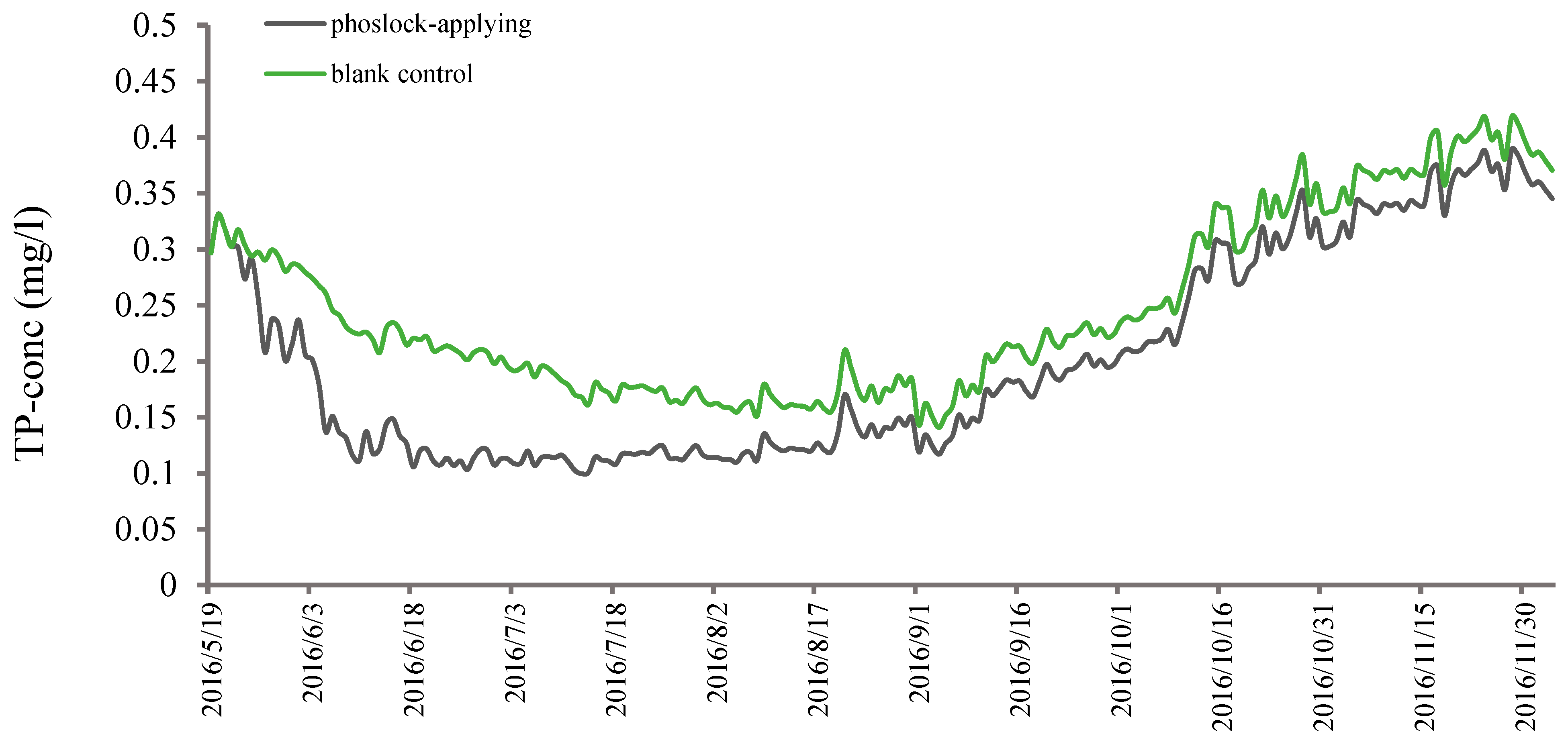
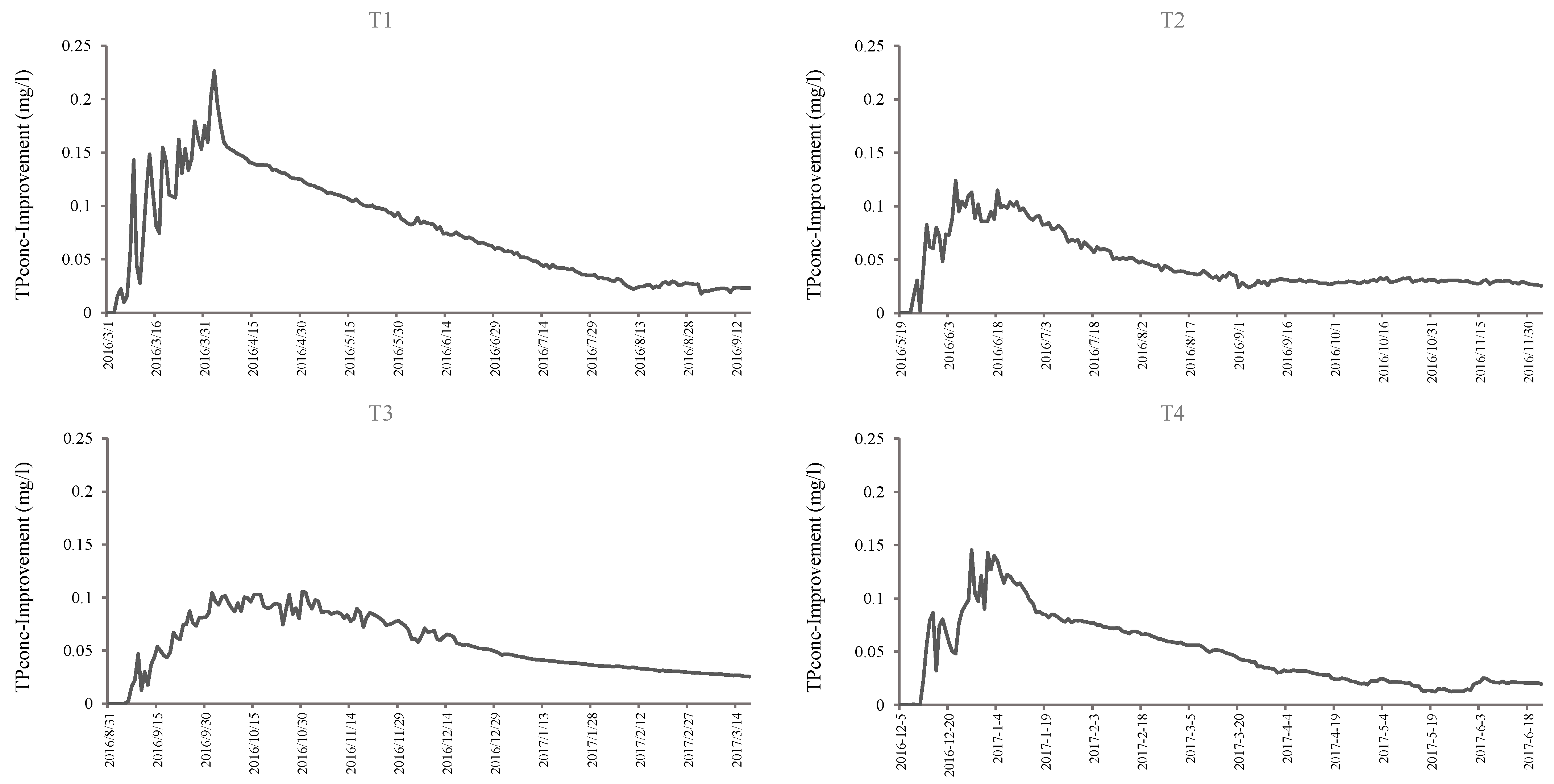
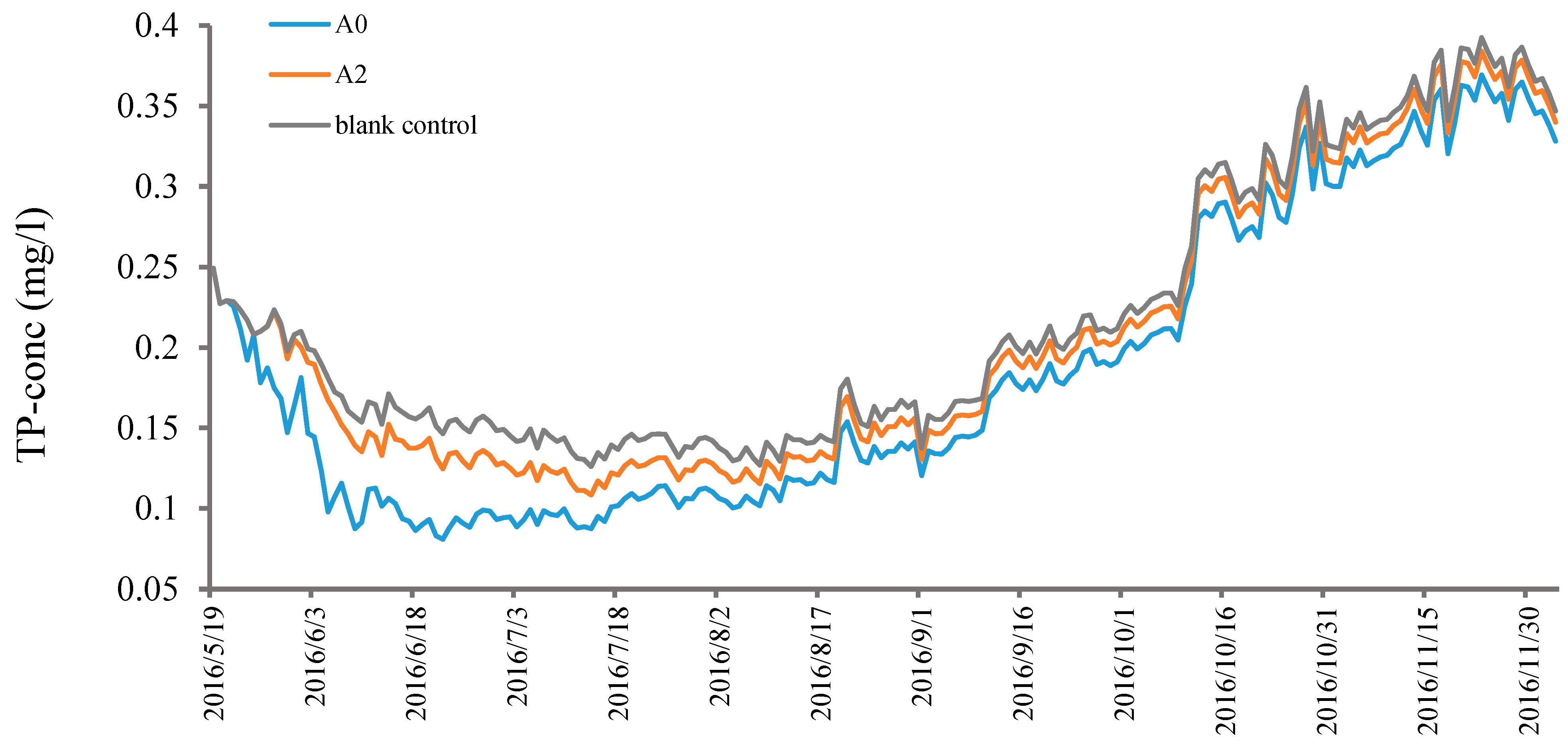
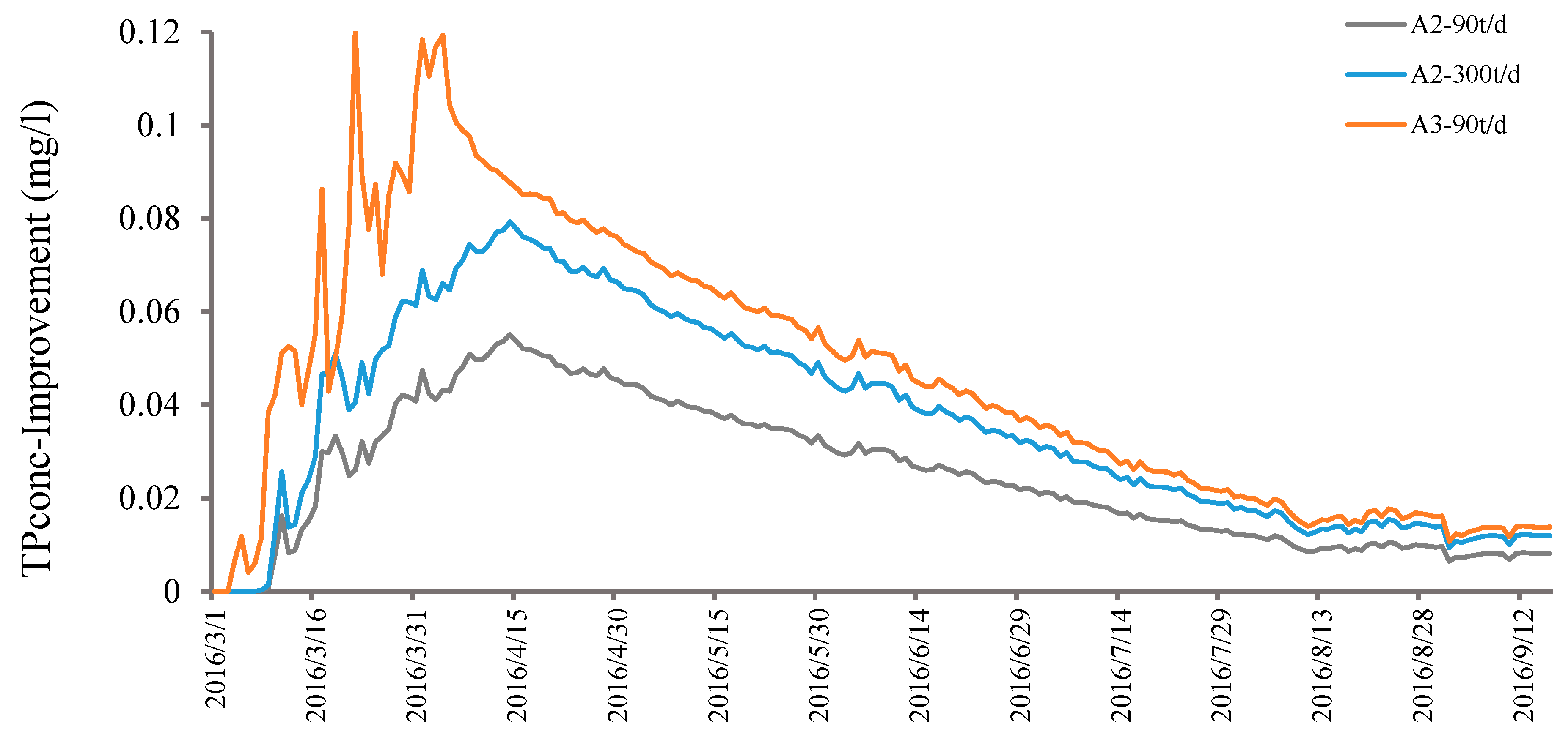
3.1. Temporal Variability of the Response

As mentioned above, the remarkable response to Phoslock happened during 200 days following the start of a 30-day release cycle. Figure 7 shows the pattern of the TP concentration time curve (TP-time) of a typical base0 scenario in T2 with a dosage of 300 t/d and position of A0. The TP-time curve for the central spot of Xingyun Lake is presented at the top of Figure 7 as a black curve, compared with the scenario of no Phoslock (green curve). In spite of fluctuations, both curves show an overall trend of decreasing followed by increasing. The TP concentration begins to decrease instantly after Phoslock application, and the gap between the black and green curves, which represents the improvement (response), reaches the maximum at the end of the release period. The gap narrows gradually from that time to 2 months later, and then remains stable for 3 or 4 months before closing. Two such curves provide key information for seeking out a goal-oriented scheme. For example, if the limit of TP concentration is 0.2 mg/L for the central spot, the scheme shown in Figure 7 is not desirable because the concentration between 7 June and 20 August 2016 was even lower than 0.15 mg/L, which means over-treatment happened. Another point is that the background (no Phoslock) TP concentration basically met the requirement between 3 July and 10 September 2016, which is relevant for identifying a release period.

Scenarios of different doses, frequencies, and time settings for the release cycle could be computed in order to find the scheme that would make the TP concentration stay at 0.2 mg/L over time, which means the least Phoslock used. Yet uncertainty or risk analysis is also needed for future planning due to incomplete predictability. This could also be done when the object is the average TP concentration or the highest TP concentration in the lake. Theoretically speaking, when all engineering design parameters are equal, the characteristics of the response (gap between curves), like the length of the stable period or the dose improvement, are determined by factors, such as exogenous input, bioavailability of phosphorus, hydrodynamic conditions, and so on. Since those factors vary with objects, there will not be a unified response for different lakes, different points in a lake, or the same point over seasons. In this sense, OOID is preferable for the traditional method because it allows applicability to specific objects.

Compared to Figure 7, Figure 8 shows the TP removal effect of Phoslock more directly. The vertical axis represents the TP improvement produced by Phoslock, which is the gap of TP concentration between Phoslock application and blank control. The horizontal axis still represents the period from the beginning of release to the 200th day and four seasons (T1-T4). The scenarios illustrated here have the same release position (A0) and dosage (300 t/d) as in Figure 7. Clearly, the four curves share some common features, but are still different in many ways. First, scenario T1 gets more improvement than the others. Second, the T1 curve fluctuates more dramatically during the release period, but instantly shows less fluctuation after that, while the T3 curve maintains the same level of fluctuation for a longer period of time. Third, the T2 curve shows a long horizontal tail, which means a stable period of improvement, and that feature is less apparent for the other curves. All of these differences display the temporal variability of response, which is relevant for designing the scheme over seasons. Since these curves are the result of complex interactions of many factors, mechanistic analysis of the driving process of temporal variability is complicated, and intuitive prediction is even less likely.

The OOID approach uncovers the information in advance by modeling, and, thus, can design an adaptive scheme, which means all the design parameters change with time. For example, if the designers already know how the TP concentration could change with time without treatment, and roughly know how the response of a Phoslock application might change with time, then they could generate scenarios based on this information. For instance, the treatment term could be divided monthly, and all the design parameters would be adjusted to monthly in the scheme. By computing and searching the cost-effective sub-scheme for each month from the monthly scenarios, we can get a dynamic scheme composed of monthly cost-effective sub-schemes. Apparently, a dynamic scheme has more potential for effectively controlling the TP concentration at required levels than a fixed scheme.

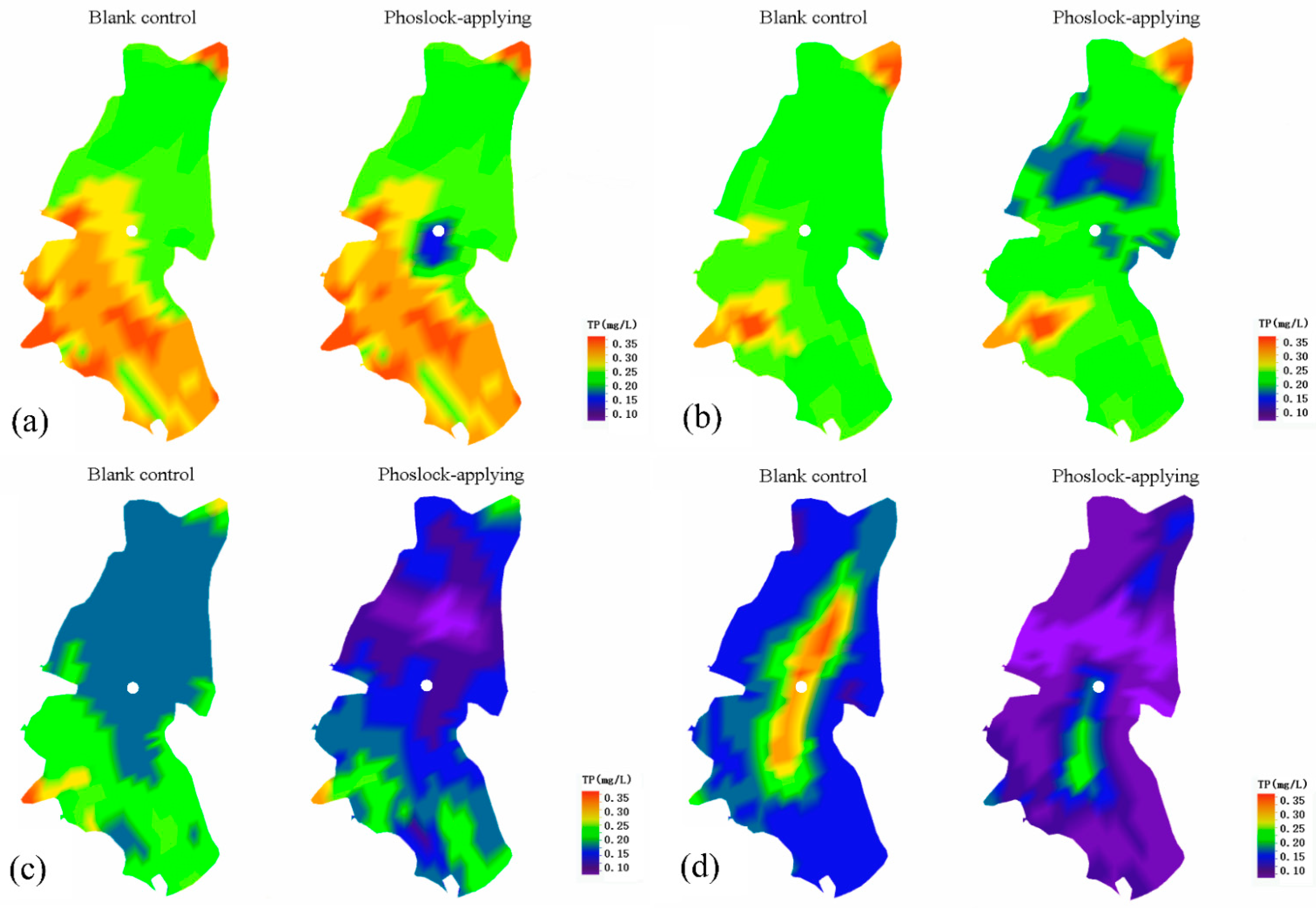
3.2. Spatial Variability of the Response

The discussion in the previous section shows how the response varies with the seasons, while this section analyzes the spatial distribution of the response. To display the process, the distribution of TP concentration over the whole lake at four moments in an assumed Phoslock-release cycle, compared with no Phoslock, is presented in Figure 9. The release cycle assumed here happened in the first season (T1), with a dosage of 300 t/d and position at A0. Clearly, the Phoslock made a low TP hollow where it merely surrounded the central spot (the white spot in the figure) on the first day of treatment, which is reasonable because the position (A0) also surrounds the central spot. However, on the 5th day, the low TP area not only expanded, but also drifted away from the central spot to the north. Thus, the low TP area no longer included the central spot. This situation remained from the 5th day to the 15th day, even though the low TP area expanded farther, while the central spot was still excluded outside the edge. On the 30th day, which is the last day of the assumed cycle, the response of TP concentration to Phoslock application could be seen throughout the lake. However, a high TP belt in the core area formed by the background (the no Phoslock scenario) partly offset the effect of Phoslock, and the central spot was finally contained in a zone with relatively high TP concentration.

It could be seen that the spatial distribution of the water quality response for Phoslock varies during the release cycle, and the low TP hollow produced by Phoslock is not necessarily close to the geometric center of all release positions. Therefore, releasing the Phoslock at places close enough to the location of interest may not always be a reliable strategy, which implies that empirical linear judgment sometimes does not work here. Actually, a full understanding of how the low TP hollow moves during or after the release cycle could be gained by modelling or fine grid monitoring, and modelling is the only way to plan treatment. Moreover, since the low TP hollow is always moving, the release positions should be adjusted over time to keep the point of interest in the hollow, which means real-time design is needed for a cost-effective operation scheme.

The spatial distribution of the response changes with the design parameters. Therefore, each scenario causes a unique time series of spatial response distribution. The release position is a kind of spatial design parameter, and is directly related to the spatial distribution of the response. In order to explore the impact of the release position on the water quality response at the point of interest, two comparative analyses were conducted, which include a comparison between internal sites and estuarine sites (Figure 10), and the cross effect of the release position and dose (Figure 11).

Two positions were set with the same dosage of 300 t/d (Figure 10): internal sites surrounding the central spot of the lake (A0) and estuarine sites (A2). Three response-time curves for the central spot are presented. Apparently, TP concentration of internal sites is always lower than estuarine sites, which proves that scenario A0 is better than A2 for the central spot. Furthermore, when Phoslock is released near the lakeshore, there is a time lag between the release and the clear response of TP concentration at the center of the lake, which could be explained by the time needed to transport it.

The curves in Figure 11 correspond to the scenarios of base0, T1, A2, 90 t/d, base0, T1, A2, 300 t/d, and base0, T1, A3, and 90 t/d. The vertical axis measures the improvement of TP concentration on the spot and the horizontal axis represents the date. As shown, the scenario of A2, 300 t/d has a better result than A2, 90 t/d, which is quite logical, as more Phoslock is applied and more phosphate is adsorbed and settled. A3, 90 t/d is also better than A2, 90 t/d, which is another example showing that internal sites have an advantage over estuarine sites. However, the curve of A3, 90 t/d being located on top of A2, 300 t/d demonstrates that sometimes the choice of the position has greater significance than the choice of dose, and the position factor might reverse the logic of dosage. Since such a large difference in dose between them exists, it also proves that the OOID approach has huge cost-saving potential.

In order to understand how the release position impacts the water quality response more comprehensively, a statistical analysis is necessary. There are 1944 generated scenarios, and 864 of them have artificial positions, which means all sets of positions are comparable for each dose level. To focus on the theme, the 864 scenarios were converted into 72 points (Figure 12) by averaging the response value for the simulation period, four seasons, and three uncertainty classifications. The graph clearly shows that the heights of A0, A4, and A3 for a certain dose are very close to each other, and the others gradually decrease in the order of A1, A6, A7, A5, and A2. More rigorous analysis reveals the following findings:

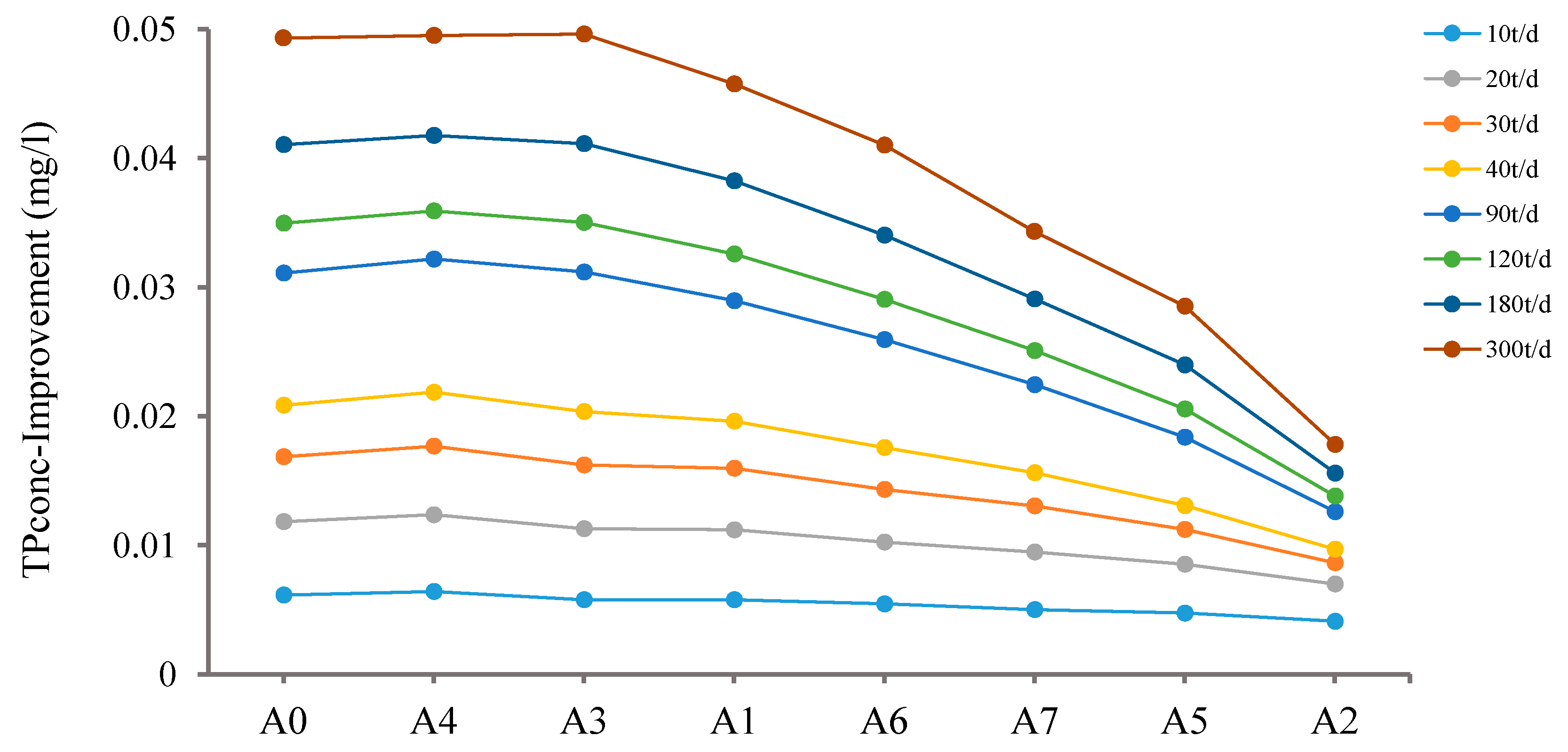
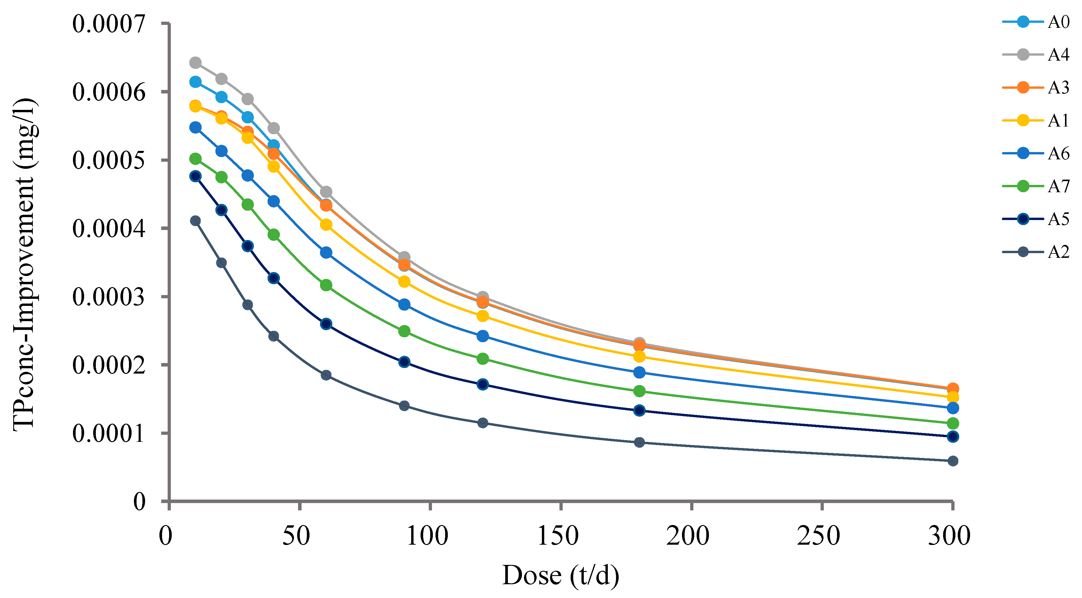
• Including more internal sites tends to get a better result. A0 and A3 have five internal sites. A4 and A1 have four internal sites. A6 has three internal sites. A5 and A7 have two internal sites, and A2 has no internal sites. Although not strictly, that sequence is basically the decreasing order in Figure 12, which, more or less, verifies the same finding discussed in Section 3.2.
• The differences in the water quality response between scenarios are not significant with a low dose, but become more clear with increased doses. The improvement of A0, A4, and A3 is not far from A2 when the dose is 10 t/d, but is more than twice as much as A2 when it is over 40 t/d.
• The TP improvement rises with the dosage for all scenarios, but the trend rate is different. For positions of A2, if the improvement of TP concentration needs to be increased from 0.01 to 0.02 mg/L, the dose has to be increased from 40 to 300 t/d (seven times). For positions of A4, it has to be increased from 20 to 40 t/d (two times).
• A4 is better than A3 when the dose does not exceed 180 t/d, but the situation is reversed when the dose is 300 t/d, and similarly for A3 and A0. Therefore, there is no unique “best scenario” here, and the best set of positions could not be determined. In practical circumstances, it still makes sense to find the best positions under more constraints, even if it may not remain the best when conditions change.

Although these findings might be valid only for this study, a common feature can be inferred that the relationship between the release position and TP improvement is nonlinear and elusive. It will definitely become more complicated when other parameters like time and uncertainty are taken into account as variables. Since the release position is a decisive parameter for the effect of Phoslock application in a large water body, the position selection becomes a difficult but very important task in designing a scheme. The use of modelling and scenario analysis is a useful method to identify good schemes or exclude inferior ones, but the problem cannot be solved once for all because the relationship changes with the boundary conditions. As discussed above, real-time OOID should be done to obtain a dynamic scheme.

3.3. Dose-Response Relationship

As Figure 10 and Figure 11 show, with other things being equal, if more Phoslock is used, more effects are produced. That seems natural, yet it is still not enough for engineering design and decision support. At least three issues are left for discussion, as follows:

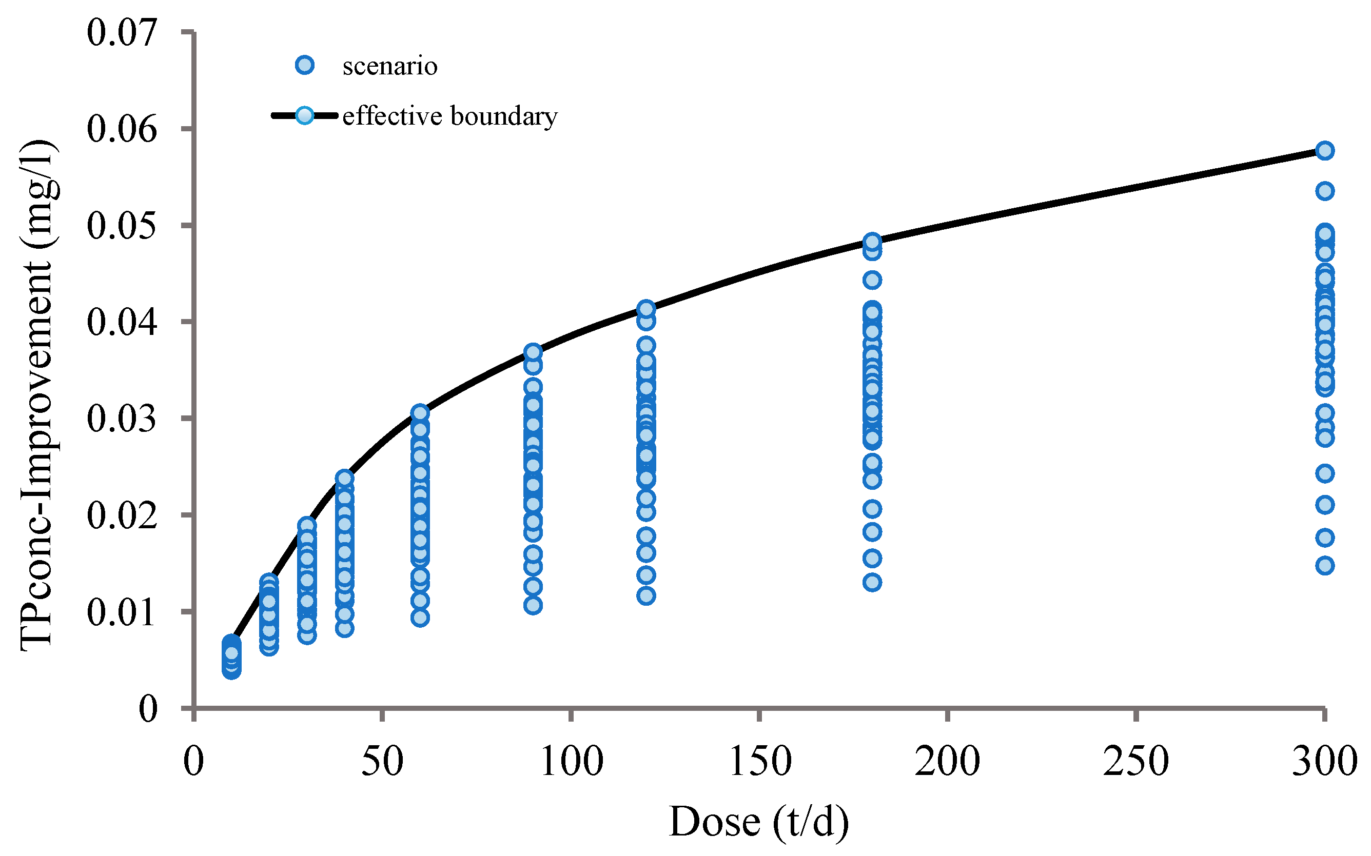
• How does the TP concentration improvement with Phoslock per weight vary with design parameters?
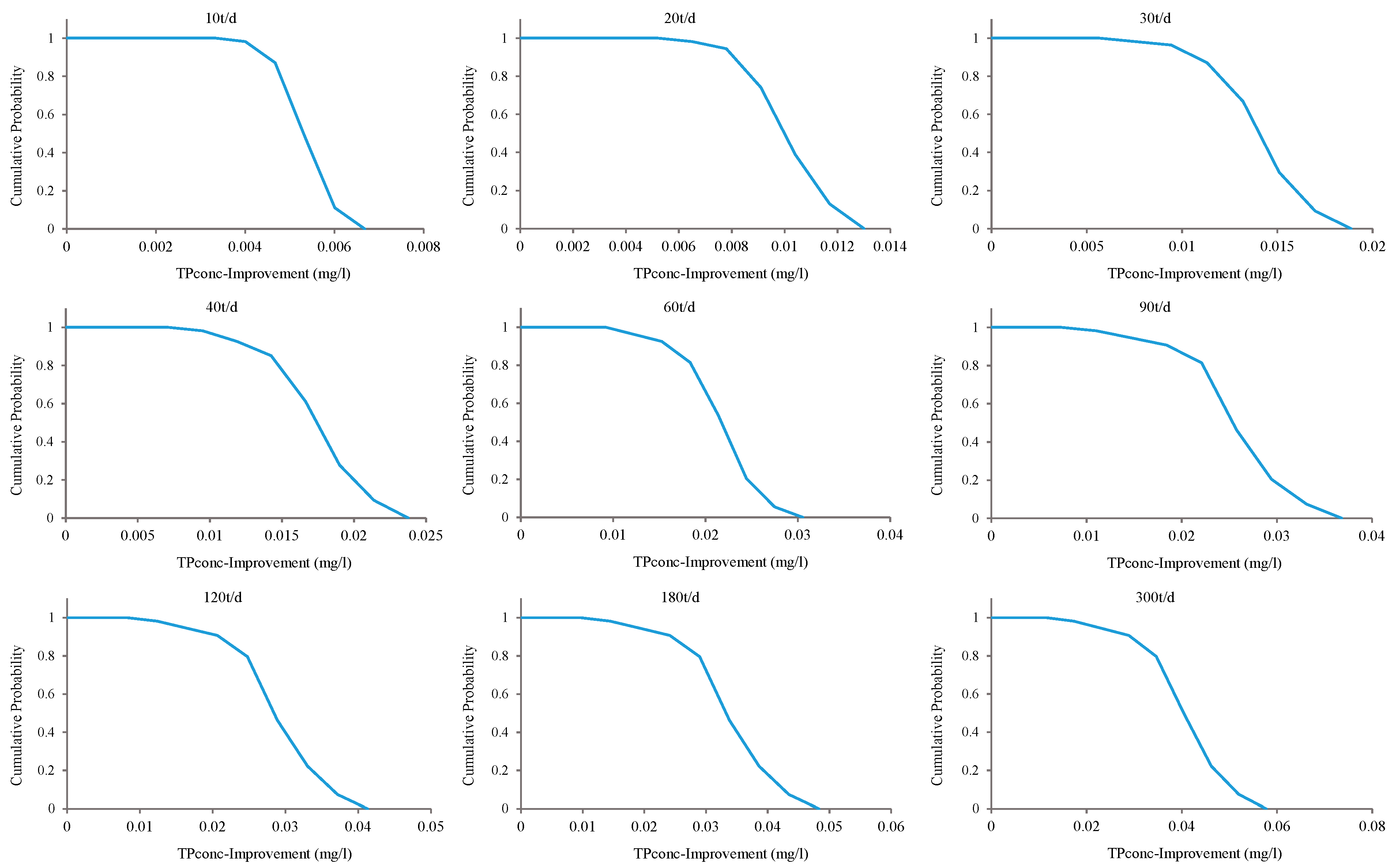
• What is the potential range of TP concentration improvement for each dose level?
• What is the probability of improving TP concentration by using a certain dose to get within the potential range?

To research these issues, more statistical analyses are needed, but it must be clear that all analyses and discussions in this section are based on the scenarios we created and the results we computed. Therefore, all the findings cannot be applied generally.

For more efficient use, it is meaningful to explore the annual improvement in the central spot per ton of Phoslock in different situations. Figure 13 shows the relationship between the efficiency of Phoslock use and combinations of scenarios and doses. The numbers on the y-axis represent improvement of TP concentration by 1 ton of Phoslock, and the x-axis represents doses. On the whole, the more Phoslock that is released, the less efficient it becomes. However, the relationship is nonlinear and the patterns of curves are not identical. Taking the comparison of A2 with A3 as an example, the steepest part of the curve, which means the sharpest decline of efficiency, presents from the very beginning to 40 t/d for A2 but from 30 to 90 t/d for A3. In addition, most curves in Figure 13 are arranged in turn, but the A3 curve intersects A0 and A4 as an exception, which additionally supports the viewpoint of no unique best scenario (This is discussed in the last section).

Knowing the potential range of TP concentration improvement could help decision-makers decide whether to continue an OOID study in depth. As a kind of decision-support project, an OOID study also comes with a cost, and a deeper study may lead to a much higher cost. Figure 14 shows the range based on statistical analysis of all 1944 scenarios. Each dot in the graph represents a mean response value of scenarios with the same position, dose level, and uncertainty classification, and, therefore, 486 dots in total. The top dot of each column in the graph represents the average response of effective scenarios for that dose level, and the line connecting these dots indicates the boundary of effectiveness. The information about the top and bottom dots and the corresponding scenarios are listed in

Table 4. Result of cost-effective analysis for each dose level.

Dose	Lowest TP Conc Improvement	Worst Scenario	Highest TP Conc Improvement	Cost-Effective Scenario
10 t/d	0.003955 mg/L	base1-A2	0.006676 mg/L	base0-A4
20 t/d	0.006356 mg/L	base1-A2	0.013003 mg/L	base0-A4
30 t/d	0.007541 mg/L	base1-A2	0.018867 mg/L	base0-A4
40 t/d	0.008267 mg/L	base1-A2	0.023763 mg/L	base0-A4
60 t/d	0.009361 mg/L	base1-A2	0.030537 mg/L	base0-A4
90 t/d	0.010631 mg/L	base1-A2	0.036812 mg/L	base0-A4
120 t/d	0.011614 mg/L	base1-A2	0.041296 mg/L	base0-A4
180 t/d	0.013029 mg/L	base1-A2	0.048266 mg/L	base0-A4
300 t/d	0.014773 mg/L	base1-A2	0.057726 mg/L	base0-A3

.

It can be seen that the range of response disproportionately increased with the dose level. The dots in each column are dense in the middle section and sparse at both ends, which shows the distribution feature. Note that, when the dose is small, the boundary curve is steep, but it gradually slows down after 40 t/d, and the inflection point is about 60 t/d. After that, the curve continues to flatten, which means that the response to the dose increment decreases. In other words, the Phoslock is used more efficiently in a low dose. The effective scenarios and worst scenarios are very constant, according to Table 4. The only exception is the cost-effective scenarios with 300 t/d, which were discussed in a previous section. By the way, it is not true that no scenario could possibly be above the effectiveness boundary shown in Figure 14, but not generated by this study. In fact, it could be further improved by a more complex scenario analysis.

According to Figure 14 and Table 4, there is a considerable range between the worst and the best. Thus, deeper OOID research is worth pursuing. Whether any further research will be done depends on the preference of researchers. If such research were done, a study like this could serve as pre-research, and, if not, a feasible scheme must be determined based on the existing research. Although the response of the best scenarios was already calculated, all of these results are based on the data acquired in the simulation period, and how those boundary conditions will change in the future is very difficult to predict. That leads to the risk of noncompliance, for the expected responses are often highly sensitive to boundary conditions. Decision-makers ought to be aware of the information about the risk. Figure 15 provides the information by computing the cumulative probability (the vertical axis represents the value of cumulative probability reduced by 1 for the convenience of observing), which is quite conservative, but useful. For example, if the goal is to reduce the TP concentration by 0.2 mg/L, any dose more than 40 t/d could achieve the goal, according to Figure 14 and Table 4. However, as explained, 40 t/d might be a risky choice in practical terms. Figure 15 shows that the probability of achieving the goal with a dose of 40 t/d is only about 20%, while, with doses of 60, 90, and 120 t/d, the probability is about 65%, 86%, and 91%, respectively. This information might be helpful in making decisions according to individual preferences.

4. Conclusions

This paper establishes a new methodology of engineering design for Phoslock application based on OOID, explores the water quality response, and analyzes the Phoslock application scheme using Xingyun Lake as a case study. By a well-quantified analysis of water quality response to Phoslock under numerous scenarios, it is found that the response curves always reflect nonlinearity and spatiotemporal heterogeneity. In addition, there is no unified response for different objects. According to the simulation, Phoslock works to reduce the TP concentration in water. With other things being equal, the more Phoslock released, the greater the decrease in TP concentration. However, the degree of improvement not only depends on the dose, but is also related to the position, season, and boundary conditions. Even lower doses could get better results than higher doses by choosing better positions for Phoslock release. The relationship between the water quality response and design parameters is nonlinear and variant, and cannot be estimated accurately by intuition or experience. This innovative method makes the water quality response correspond to a certain predictable measure, and a cost-effective scheme for a specific goal could be identified based on it. The study proves that the OOID approach could be more reliable and accurate than the traditional design method, and has huge cost-saving potential. Surely, this new methodology could help decision-makers find advisable schemes for applying Phoslock based on their preferences.

Although the methodology proposed here can be applied to other objects, the results of cost-effective analysis cannot be generally applied, and even for the same object, the results need to be updated periodically due to the ever-changing boundary conditions. With OOID, nothing is once for all. This study is only the beginning of research on OOID. Propositions such as more sophisticated scenario analysis, multiform goals, and real-time operational design are worth exploring. Apart from Phoslock, which can only control phosphorus, treatment technologies like dredging [45] and biomanipulation [23] have multiple influences on lake systems. In order to calculate the comprehensive water ecology response and seek out advisable treatment schemes, new tools are needed, such as a coupled physical/ecological model [19], which deserves further research. Moreover, no single measure or technology can cope with eutrophication. A combination of technologies is often required. For example, measures like Phoslock release might not work as usual during outbreaks of algal blooms, and technologies like algae flocculation [8,9] and oxygen nanobubbles [10] are likely needed to alleviate the harmful effects. For scenarios that include multiple technologies, greater enhancement can be expected by improving the scheme using the OOID method. Finally, as mentioned at the beginning of this paper, lake pollution control can be categorized as an external source control or in-lake restoration. A specific goal, such as reducing TP, can be achieved by both land source control and lake in situ control. It is crucial to compare the pros and cons between the best management practices or phosphorus recovery technologies in treatment plants [7] and phosphate absorption in lakes, which will show the big picture of decision support for lake recovery.

References

- Hayes, N.M.; Vanni, M.J. Microcystin concentrations can be predicted with phytoplankton biomass and watershed morphology. Inland Waters 2018, 8, 273–283. [Google Scholar] [CrossRef]
- Jing’an, M.; Hongqing, L. On eutrophication of rivers, lakes and reservoirs at home and abroad. Resour. Environ. Yangtze River Basin 2002, 11, 575–578. (In Chinese) [Google Scholar]
- Ministry of Ecology and Environment of the People’s Republic of China [EB/OL]. Available online: http://www.mee.gov.cn/hjzl/sthjzk/zghjzkgb/ (accessed on 2 June 2020). (In Chinese)
- Beusen, A.H.W.; Bouwman, A.F.; Van Beek, L.P.H.; Mogollón, J.M.; Middelbur, J.J. Global riverine N and P transport to ocean increased during the 20th century despite increased retention along the aquatic continuum. Biogeosciences 2016, 13, 2441–2451. [Google Scholar] [CrossRef]
- Huang, J.; Xu, C.; Ridoutt, B.G.; Wang, X.; Ren, P. Nitrogen and phosphorus losses and eutrophication potential associated with fertilizer application to cropland in China. J. Clean. Prod. 2017, 159, 171–179. [Google Scholar] [CrossRef]
- Li, X.Y.; Li, H.P.; Jiang, S.Y.; Ma, P.; Lai, X.; Deng, J.C.; Chen, D.Q.; Geng, J.W. Temporal-spatial variations in nutrient loads in river-lake system of Changdang Lake catchment during 2016–2017. Environ. Sci. 2020, 41, 4042–4052. (In Chinese) [Google Scholar]
- Daneshgar, S.; Callegari, A.; Capodaglio, A.G.; Vaccari, D. The Potential Phosphorus Crisis: Resource Conservation and Possible Escape Technologies: A Review. Resour. Basel 2018, 7, 37. [Google Scholar] [CrossRef]
- Zhang, H.; Shang, Y.; Lyu, T.; Chen, J.; Pan, G. Switching Harmful Algal Blooms to Submerged Macrophytes in Shallow Waters Using Geo-engineering Methods: Evidence from a N-15 Tracing Study. Environ. Sci. Technol. 2018, 52, 11778–11785. [Google Scholar] [CrossRef]
- Pan, G.; Miao, X.; Bi, L.; Zhang, H.; Wang, L.; Wang, L.; Wang, Z.; Chen, J.; Ali, J.; Pan, M.; et al. Modified Local Soil (MLS) Technology for Harmful Algal Bloom Control, Sediment Remediation, and Ecological Restoration. Water 2019, 11, 16. [Google Scholar] [CrossRef]
- Zhang, H.; Lyu, T.; Bi, L.; Tempero, G.; Hamilton, D.P.; Pan, G. Combating hypoxia/anoxia at sediment-water interfaces: A preliminary study of oxygen nanobubble modified clay materials. Sci. Total Environ. 2018, 637–638, 550–560. [Google Scholar] [CrossRef]
- Oglesby, R.T.; Edmondson, W.T. Control of eutrophication. J. Water Pollut. Control. Fed. 1966, 38, 1452. [Google Scholar]
- Welch, E.B. The dilution-flushing technique in lake restoration. Water Resour. Bull. 1981, 17, 558–564. [Google Scholar] [CrossRef]
- Jeppesen, E.; Søndergaard, M.; Meerhoff, M.; Lauridsen, T.L.; Jensen, J.P. Shallow lake restoration by nutrient loading reduction—Some recent findings and challenges ahead. Hydrobiologia 2007, 584, 239–252. [Google Scholar] [CrossRef]
- Hu, L.; Hu, W.; Zhai, S.; Wu, H. Effects on water quality following water transfer in Lake Taihu, China. Ecol. Eng. 2010, 36, 471–481. [Google Scholar] [CrossRef]
- Liu, Y.; Wang, Y.; Sheng, H.; Dong, F.; Zou, R.; Zhao, L.; Guo, H.; Zhu, X.; He, B. Quantitative evaluation of lake eutrophication responses under alternative water diversion scenarios: A water quality modeling based statistical analysis approach. Sci. Total Environ. 2014, 468–469, 219–227. [Google Scholar] [CrossRef]
- Camacho, R.A.; Zhang, Z.; Chao, X. Receiving Water Quality Models for TMDL Development and Implementation. J. Hydrol. Eng. 2019, 24, 04018063. [Google Scholar] [CrossRef]
- Mohamoud, Y.; Zhang, H. Applications of Linked and Nonlinked Complex Models for TMDL Development: Approaches and Challenges. J. Hydrol. Eng. 2019, 24, 11. [Google Scholar] [CrossRef]
- You, X.-Y.; Zhang, C.-X. On improvement of water quality of a reservoir by optimizing water exchange. Environ. Prog. Sustain. Energy 2018, 37, 399–409. [Google Scholar] [CrossRef]
- Capodaglio, A.G.; Boguniewicz, J.; Llorens, E.; Salerno, F.; Copetti, D.; Legnani, E.; Buraschi, E.; Tartari, G. Integrated lake/catchment approach as a basis for the implementation of the WFD in the Lake Pusiano watershed. In Proceedings of the River Basin Management—Progress Towards Implementation of the European Water Framework Directive, Budapest, Hungary, 19–20 May 2005. [Google Scholar]
- Zhang, F.; Zhang, M.; Gao, L.; Li, K. Pilot-scale test of treating eutrophication water in Chaohu lake using biological pond. Environ. Eng. 2009, 27, 9–11. (In Chinese) [Google Scholar]
- Wang, W.-H.; Wang, Y.; Sun, L.-Q.; Zheng, Y.-C.; Zhao, J.-C. Research and application status of ecological floating bed in eutrophic landscape water restoration. Sci. Total Environ. 2020, 704, 135434. [Google Scholar] [CrossRef]
- Chen, X.; Chen, X.; Zhao, Y.; Zhou, H.; Xiong, X.; Wu, C. Effects of microplastic biofilms on nutrient cycling in simulated freshwater systems. Sci. Total Environ. 2020, 719, 137276. [Google Scholar] [CrossRef] [PubMed]
- Liu, H.; Cao, L.; Xu, G.J.; Wang, T.J. Study on the remediation of eutrophic water by enhanced biomanipulation of Daphnia magna. Environ. Sci. Technol. 2020, 43, 156–161. (In Chinese) [Google Scholar]
- Li, X.; Zhang, Z.; Xie, Q.; Yang, R.; Guan, T.; Wu, D. Immobilization and Release Behavior of Phosphorus on Phoslock-Inactivated Sediment under Conditions Simulating the Photic Zone in Eutrophic Shallow Lakes. Environ. Sci. Technol. 2019, 53, 12449–12457. [Google Scholar] [CrossRef] [PubMed]
- Yang, Y.Q.; Chen, J.A.; Wang, J.F.; Yan, Z. Research progress of sediments phosphorus in-situ inactivation. Adv. Earth Sci. 2013, 28, 674–683. (In Chinese) [Google Scholar]
- Copetti, D.; Finsterle, K.; Marziali, L.; Fabrizio, S.; Gianni, T.; Grant, D.; Kasper, R.; Bryan, S.; Spearse, M.; Ian, J.; et al. Eutrophication management in surface waters using lanthanum modified bentonite: A review. Water Res. 2016, 97, 162–174. [Google Scholar] [CrossRef] [PubMed]
- Liu, Y.G.; Tian, K.; Winks, A. Phoslock, a Soluble Phosphorus Binding Technology, Application in Lake Dianchi Eutrophic Water Purification. In Proceedings of the 2009 International Conference on Environmental Science and Information Application Technology, Wuhan, China, 4–5 July 2009. [Google Scholar]
- Pan, M.; Lyu, T.; Zhang, M.; Zhang, H.; Bi, L.; Wang, L.; Chen, J.; Yao, C.; Ali, J.; Best, S.; et al. Synergistic Recapturing of External and Internal Phosphorus for In Situ Eutrophication Mitigation. Water 2019, 12, 2. [Google Scholar] [CrossRef]
- Wei, H.; Chai, L. Non-linear dynamic characteristics of phosphorus cycle and eutrophication. Hupo Kexue 2006, 18, 557–564. (In Chinese) [Google Scholar]
- Liu, Y.; Wang, Y.L.; Sheng, H.; Dong, F.F.; Zou, R.; Zhao, L.; Guo, H.C.; Zhu, X.; He, B. Lake eutrophication responses modeling and watershed management optimization algorithm: A review. Hupo Kexue 2021, 33, 49–63. (In Chinese) [Google Scholar]
- Zou, R.; Zhou, J.; Liu, Y.; Zhu, X.; Zhao, L.; Yang, P.-J.; Guo, H.-C. An object-oriented intelligent engineering design approach for lake pollution control. Huan Jing Ke Xue= Huanjing Kexue 2013, 34, 892–899. [Google Scholar] [PubMed]
- Li, Z.-F.; Liu, H.-Y.; Li, Y. Review on HSPF model for simulation of hydrology and water quality processes. Huanjing Kexue 2012, 33, 2217–2223. (In Chinese) [Google Scholar] [PubMed]
- Arnold, J.G.; Moriasi, D.N.; Gassman, P.W.; Abbaspour, K.C.; White, M.J.; Srinivasan, R.; Santhi, C.; Harmel, R.D.; Van Griensven, A.; Van Liew, M.W.; et al. SWAT: Model Use, Calibration, and Validation. Trans. ASABE 2012, 55, 1491–1508. [Google Scholar] [CrossRef]
- Yuan, L.; Sinshaw, T.; Forshay, A.K.J. Review of Watershed-Scale Water Quality and Nonpoint Source Pollution Models. Geosciences 2020, 10, 25. [Google Scholar] [CrossRef] [PubMed]
- DHI. Mike she volume 1: User guide. The experts in water environments. DHI Softw. Licence Agreem. 2017, 27, 91–95. [Google Scholar]
- DHI. MIKE 21 & MIKE 3 Hydrodynamic and Transport Scientific Documentation. Danish Hydraulic Institute. 2017. Available online: https://manuals.mikepoweredbydhi.help/2020/Coast_and_Sea/MIKE_FM_ELOS_2D.pdf (accessed on 20 February 2021).
- Hamrick, J.M. A Three-Dimensional Environmental Fluid Dynamics Computer Code: Theoretical and Computational Aspects; Special paper 317; The College of William and Mary, Virginia Institute of Marine Science: Williamsburg, NY, USA, 1992. [Google Scholar]
- Delft3D-FLOW User Manual, 710. Available online: https://usermanual.wiki/Pdf/Delft3DFLOWUserManual.885467064/help (accessed on 20 February 2021).
- D-Water Quality User Manual, 414. Available online: https://content.oss.deltares.nl/delft3d/manuals/D-Water_Quality_User_Manual.pdf (accessed on 20 February 2021).
- DHI. MIKE 3 Flow Model User Guide and Scientific Documentation. Danish Hydraulic Institute. 2017. Available online: https://manuals.mikepoweredbydhi.help/2017/Coast_and_Sea/MIKE_321_FM_Scientific_Doc.pdf (accessed on 20 February 2021).
- Gao, C.; Yu, J.; Min, X.; Cheng, A.; Hong, R.; Zhang, L. Heavy metal concentrations in sediments from Xingyun lake, southwestern China: Implications for environmental changes and human activities. Environ. Earth Sci. 2018, 77, 1–13. [Google Scholar] [CrossRef]
- Wang, S.; Dou, H. Chinese Lakes; Science Press: Beijing, China, 1998; p. 580. (In Chinese) [Google Scholar]
- Liu, Y.; Chen, G.; Hu, K.; Shi, H.; Huang, L.; Chen, X.; Lu, H.; Zhao, S.; Chen, L. Biological responses to recent eutrophication and hydrologic changes in Xingyun Lake, southwest China. J. Paleolimnol. 2017, 57, 343–360. [Google Scholar] [CrossRef]
- Zheng, T.; Zu, Z.; Xiao, Z.; Ze, G.; Jun, P.; Feifeiet, L. Water quality change and humanities driving force in Lake Xingyun, Yunnan Province. Hupo Kexue 2018, 30, 79–90. (In Chinese) [Google Scholar]
- Zhong, J.; Wen, S.; Zhang, L.; Wang, J.; Liu, C.; Yu, J.; Zhang, L.; Fan, C. Nitrogen budget at sediment–water interface altered by sediment dredging and settling particles: Benefits and drawbacks in managing eutrophication. J. Hazard. Mater. 2021, 406, 124691. [Google Scholar] [CrossRef]