1. Introduction
Sediment transport has a considerable impact on river processes, in part defining river morphology [
1] and influencing water quality [
2]. River flow hydraulics and sediment transport together are processes that determine river behavior [
3]. Sediment transport has been studied in detail by [
4,
5,
6,
7], and [
8] among others. However, most studies have been performed with fine sediment (1.56 <
d50 (mm) < 28.6) and mild slopes (~0% <
So < 2%) [
9,
10,
11]. On the other hand, steep rough-bedded channels constitute the main component of mountainous drainage systems. These channels are the principal source of sediment to milder slope downstream channels [
12]. Thus, sediment transport in steep channels influences processes like landscape morphology evolution, sediment routing during hydrological events, and flow hydraulics in river systems. To determine the development of these processes, understanding and knowledge of bedload transport in steep channels must be improved. Sediment transport in steeper channels with coarser material is a complex process. The continuously changing driving forces, basin sediment production, and riverbed conditions, such as high gradients and elements of roughness, result in a high uncertainty in the quantification of sediment transport rates [
1,
13,
14]. The uncertainty reported can reach some orders of magnitude [
12,
15,
16]. The presence of large diameter particles in the stream causes changes in flow hydraulics (e.g., velocity profile) and turbulence intensity, hydraulic jumps, areas of flow acceleration and deceleration, and high spatial variability of boundary shear stress [
17,
18]. Some equations have been proposed to describe bedload transport rates, movement thresholds, and channel roughness of steep channels with coarse sediment [
19]. Smart [
11] developed aA relation for slopes ranging from 3% to 20% was developed by [
11]. Moreover, the performance of this model was found to be better than other similar models in the case of high slopes [
20]. More recent studies [
21], Yager et al. [
22] have considered the typical features of steep channels such as wide grain size distribution ranging from large almost immobile boulders to finer more mobile sediments, the effective stress that causes sediment movement (which is smaller than the total shear stress), and the reduced amount of mobile sediment. However, the variation and randomness of parameters like grain size distribution, spatial distribution of immobile grains, and the streambed conditions, need to be analyzed as fundamental parameters for bedload transport [
22]. Additionally, Juez et al. [
23] found that better predictions of bedload transport rates are obtained when gravity projections, which become more significant due to high slopes, are considered in bedload transport models. Therefore, as the first approach to developing a consistent procedure to capture the high variability present in natural rivers, this work presents the validation of an experimental methodology to determine bedload transport rates for steep slopes (3% to 5%) using sediments with both uniform sizes and with a grain size distribution.
2. Background
Bed load sediment transport is defined by Garcia [
24] as the process through which streams, rivers, or bed material of artificial channels is transported. Additionally, Bagnold [
25] defined the bed load transport as that which occurs in continuous contact with the bed surface and is driven just by gravity. On the other hand, Einstein [
6,
26] defined bedload transport as the transport that occurs by sliding, rolling, and jumping over the bed surface (saltation). These processes occur in a thin layer (two times sediment diameter approximately), called the bed load layer. Sediment will be transported when the acting boundary shear stress exceeds a critical value. Additionally, recent studies have shown that impulse may be a more appropriate parameter for determining particle motion threshold [
27,
28,
29,
30,
31,
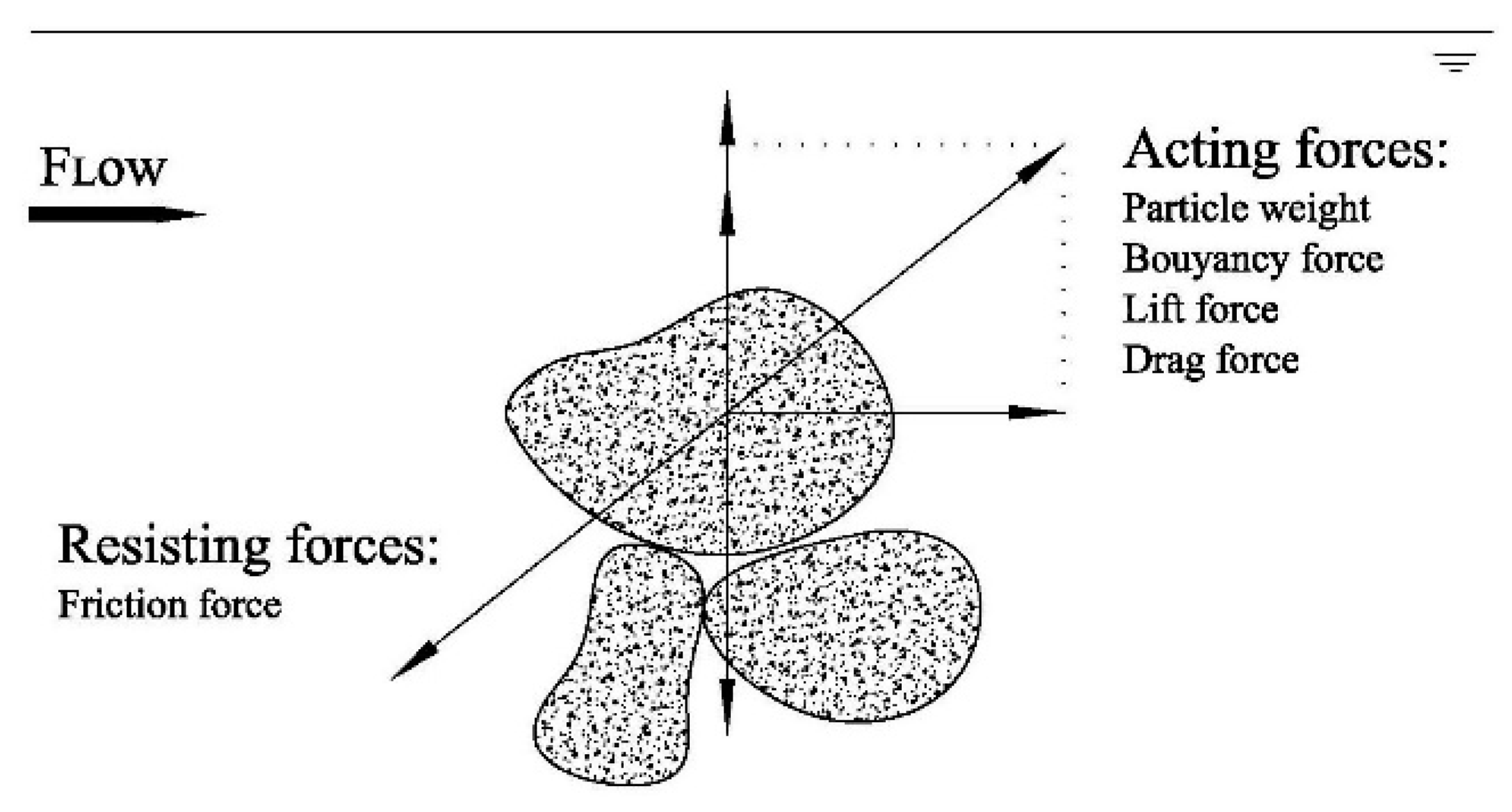
32]. Generally, particle motion will begin when the acting forces, including sediment particle weight FW, buoyancy force FB, lift force FL, and drag force FD, overcome the resisting force, FR, as illustrated in
Figure 1.
The limit condition, when acting forces equal resisting forces, defines the threshold of motion. The exact definition of this threshold condition is not possible; however, some qualitative descriptions have been proposed but, due to the high variability of the flow conditions under which particle movement is initiated, a universal condition cannot be established for movement threshold [
33]. As an attempt to characterize particle initiation of motion, some approximations have been derived through experimentation [
34]. It has been established that the transport threshold is a function of several dimensionless parameters as follows.
where
τo is the boundary shear stress,
ρs the sediment density,
ρ the fluid density,
ds the sediment diameter,
g the gravitational acceleration,
s the sediments relative density and
μ the fluid viscosity. The first term represents a stability parameter,
τ*, to analyze threshold conditions. This parameter represents the dimensionless boundary shear stress [
5].
The critical value of the stability parameter, τ*c, defines the boundary shear stress for which motion begins. In other words, sediment transport starts when τ* > τ*c. The critical Shields parameter (τ*c) is a function of the shear Reynolds number or particle Reynolds number (Rep).
The boundary shear stress can also be expressed in terms of the shear velocity,
Vsh, defined as
Vsh = √(τo/ρ). Expressing the above function in terms of shear velocity the following final function results.
The first term in this function has the form of Froude number. The second term is the relative density and the third term is a form of Reynolds number known as the shear Reynolds number [
2,
34].
Shields [
5] developed an experimental procedure to estimate the relation between the critical Shields parameter and the shear Reynolds number. This relation was proposed as a diagram now known as the Shields diagram. Based on the Shields diagram many studies have been conducted to overcome inconsistencies that have been reported by several authors [
35,
36] and have determined different values for the critical value of the Shields parameter or movement threshold [
37,
38,
39,
40]. However, the Shields diagram is still widely used to define threshold conditions.
Once the threshold of sediment movement has been established, determining the rate of sediment movement or transport is the next step to characterize the sediment transport process. The relations for bedload transport can be presented as a dimensionless function as follows.
where
R is the sediment submerged specific gravity,
R = (ρs − ρ)/ρ, and
q* is the dimensionless bedload transport rate, also known as the Einstein bedload number. It is expressed as:
Here,
qs is the volumetric bedload transport rate per unit width (m
3/s/m or m
2/s) and
go represents the gravity vector projection (
go = cos
2 (
φ)) [
23]. Angle
φ corresponds to the inclination of the bed with respect to the horizontal. This projection has been defined by Juez et al. [
41] to include effects of steep slopes on pressure distribution and friction, considering that the gravity vector projection has improved the prediction capacity of the sediment transport models with respect to the estimations using gravity vector directly [
2,
20].
Essentially, the bedload transport rate can be defined as the product of the sediment velocity,
Vs, mean sediment concentration,
Cs, and bedload layer thickness,
δs [
24].
However, many methods have been used to estimate bedload transport rates. Given that bedload transport can be approached as a deterministic or a probabilistic problem, several models for its quantification have been obtained based on four basic principles. Bed shear stress, flow discharge, stochastic functions for sediment movement, and stream power have been considered as the fundamental parameters on which bedload depends [
2,
4,
26,
42,
43]. Thus, some mathematical models have been proposed to estimate bedload transport rate. In this study, the most representative formulae for steep channels with coarse sediment have been chosen to perform a comparative analysis and evaluate the validity of the experimental procedures proposed.
Table 1 presents the selected equations and their applicability ranges [
34].
3. Experimental Procedure
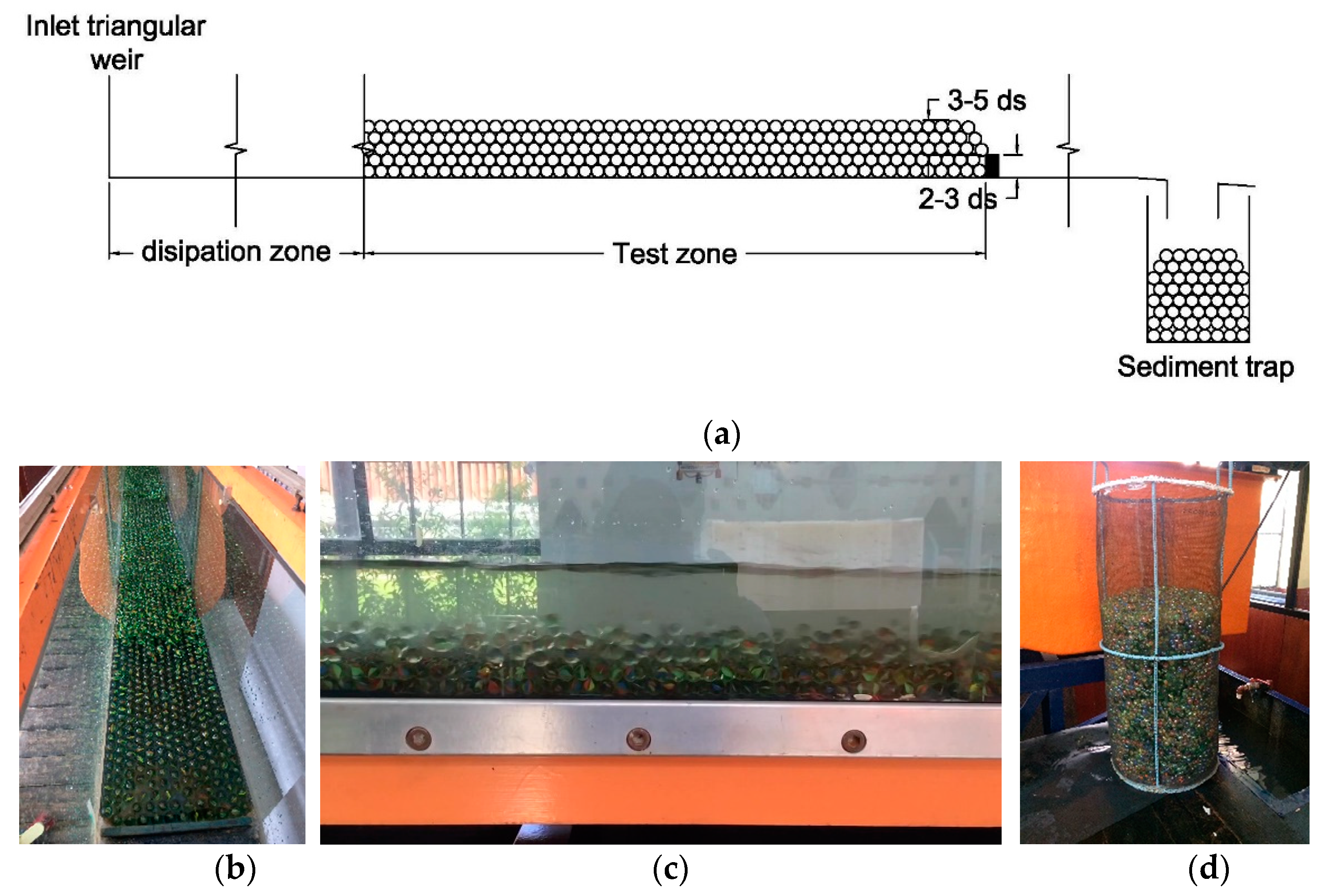
The experimental investigation presented here was performed at the Hydraulics and Fluid Dynamics Laboratory (University of Cuenca, Faculty of Engineering). The experiments were conducted in a 12 m long rectangular tilting flume with a width of 0.30 m and a height of 0.45 m. Water was provided by a recirculation system and the flow was controlled with a triangular weir located at the flume entrance. Discharge measurements were estimated from the calibrated head-discharge relationship (maximum error 5%) and the measured water head (point gauge with a resolution of ± 0.1 mm). The discharge range was defined to analyze the transport behavior under high and low flows considering the system capacity. The range of experimental settings is summarized in
Table 2. Sediment was simulated with glass spheres (specific gravity = 2766.81 kg/m
3) of different diameters. For each simulation, the channel gradient was set first. The sediment was placed at a total length of about 5 m at the beginning of each run. A first layer of immobile sediment, of a thickness from 2 to 3
ds, was located on the bottom of the channel. Over this immobile layer, a layer of mobile sediment was placed, with a thickness of from 3 to 5
ds. A schematic of the flume and sediment configuration is shown in
Figure 2. Once uniform flow was established, the simulation time began. Sediment transported before this is not considered for the transport rate calculation. No sediment was fed at the inlet of the simulation zone because the transport rates obtained from a set of calibration experiments showed no dependence on sediment feed rate. Each run was considered complete when the total mobile sediment layer was transported. At the end of the channel, transported sediment was collected in a sediment trap. For each simulation, discharge, flow depth, and water temperature were measured. An experimental configuration consisted of a discharge, a channel slope, and a sediment type. Three experiments were performed for each configuration with different running times to verify the validity of the transport rates obtained. Water temperature was measured at the beginning and at the end of each simulation. The profile length required to reach uniform flow conditions was calculated for each experiment. The test section was located 3.5 m downstream from the inlet weir. The maximum length, based on flow and geometry conditions, that is needed to reach normal depth (from critical to normal flow depth in the downstream direction and vice versa in the upstream direction) is 3 m. The distance from the end of the test section to the outlet was 3.5 m. Thus, normal depth was ensured by placing the test zone downstream far enough to reach uniform conditions for steep slopes and upstream enough for mild slopes. The flow started in a hydraulic jump downstream of the inlet weir and ended in a free fall. Normal depth was verified at the beginning, at the middle and at the end of the test section. Sediment collected in each run was dried and weighed to determine the transport rate by dividing the weight of the transported sediment by the collection time.
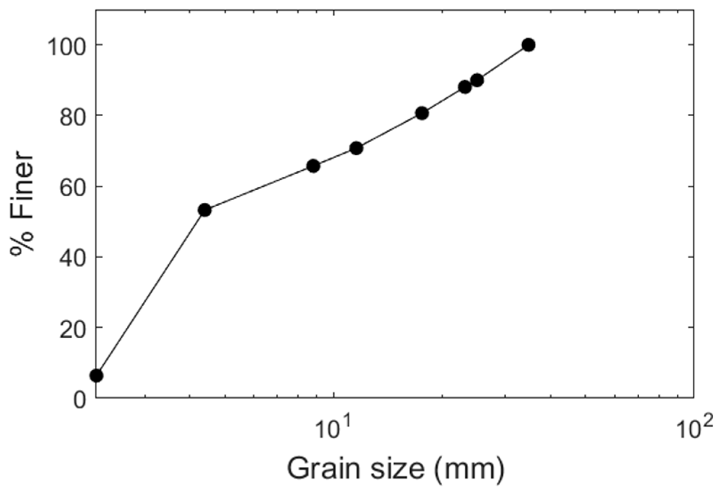
The experiment was carried out for four cases: A, B, C, and D, based on sediment characteristics. Case A corresponds to the experiments performed with spheres of a uniform diameter of 10 mm. Case B consisted of spheres of 15 mm and Case C of spheres of 25 mm. These sediment sizes were chosen to replicate the coarser range of sizes considered in previous studies. Case D was performed with a typical mountainous river grain size distribution that was built with the particle diameters used in the other cases.
Figure 3 shows the grain size distribution for Case D. The median diameter
d50 for this grain size distribution is 53.10 mm. In the present study
d84 is considered as the characteristic diameter with
d84 = 21.70 mm.
5. Results and Discussion
The experiments performed with the combinations of the independent variables presented in
Table 2 gave a total of 140 values for transport rates. A correlation analysis was performed between the dependent variable bedload transport rate and the measured flow hydraulics parameters in dimensionless form.
Table 3 presents the range of variation of the correlation coefficients of a simple linear regression of each parameter, with bedload transport rate for the four cases simulated, to determine their individual correlation with transport rate. In the case of slope, the linear regressions were performed maintaining a constant discharge.
As can be seen in
Table 3, the correlation coefficients obtained have similarly high values for all the variables considered. Prioritizing measured primary variables, the variables selected as the parameters a, b, and c in Equation (7) are dimensionless discharge, dimensionless flow depth, and slope, respectively. Dimensionless discharge has been selected as the flow parameter. Dimensionless flow depth (also defined as relative submergence
Y/ds) has been selected, since as slope increases it decreases, meaning particle diameter has a higher influence on flow and sediment transport mechanics [
52,
53]. Slope has mainly been neglected in the study of hydraulic processes under the assumption of mild slopes. Even though in bedload sediment transport it is indirectly included for the calculation of other parameters such as bed shear stress, in this case, due to its high values, slope becomes an important parameter that must be considered directly as an independent variable.
A multiple correlation analysis was performed for all the simulation cases defined (A, B, C, and D). In
Table 4 the estimated parameters of Equation (7) for each case with multiple regression are presented. The statistics of the multiple regression for each simulation case are shown in
Table 5.
As can be verified in
Table 5, all cases result in an acceptable goodness of fit. However, since Case D is more representative of field conditions, it is assumed to describe the processes observed in laboratory experimentation. Thus, the mathematical model is defined as follows.
Even though Equation (12) is expressed in dimensionless form and Equation (7) in dimensional when they are compared some similarities can be reported. Both equations include a flow parameter. In case of Equation (12) this is dimensionless discharge. For Equation (7) it is particle velocity that is a function of discharge and particle size both parameters included in dimensionless discharge. Equation (7) considers the bedload layer thickness. This can be comparable to dimensionless flow depth (Y/ds) in the denominator in Equation (12). If it is inverted and put in the numerator it becomes a comparable parameter to bedload layer thickness. An important difference is that Equation (12) considers slope as an independent variable and Equation (7) does not. From the correlation of between slope and bedload transport rate, it has been shown that slope, due to its high values, has an important impact on transport rates. Therefore, its inclusion in Equation (12) represents an improvement over Equation (7).
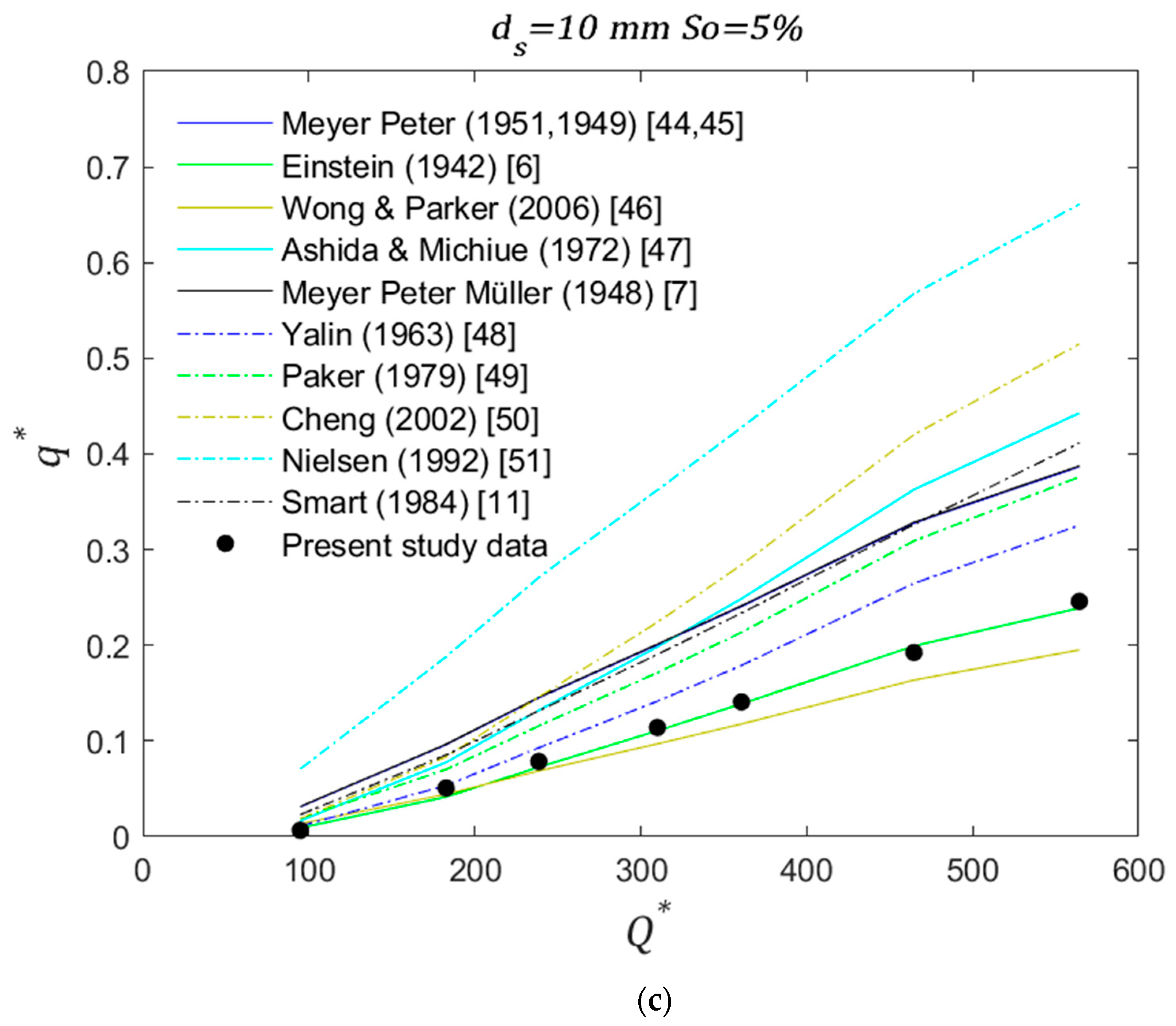
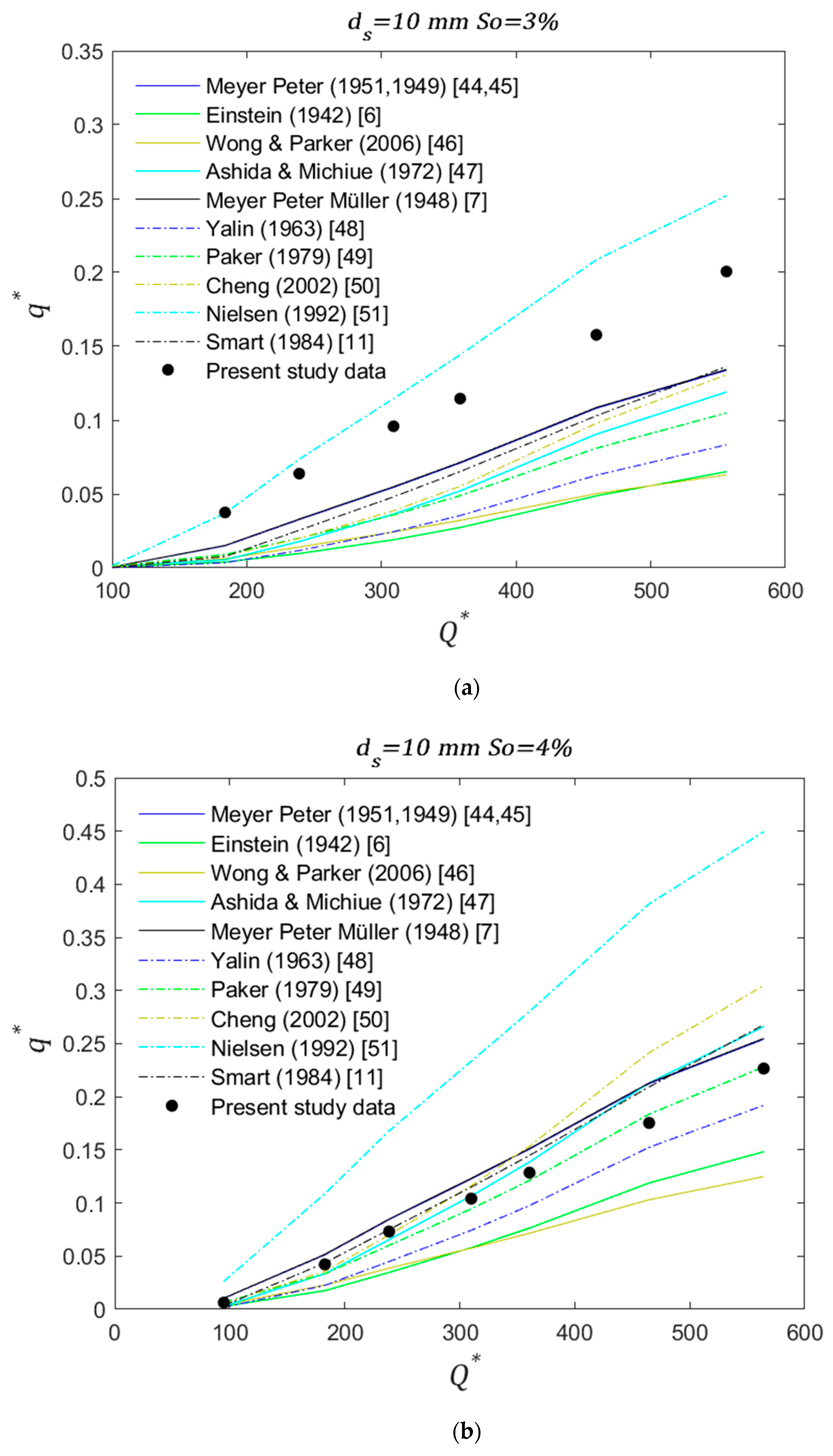
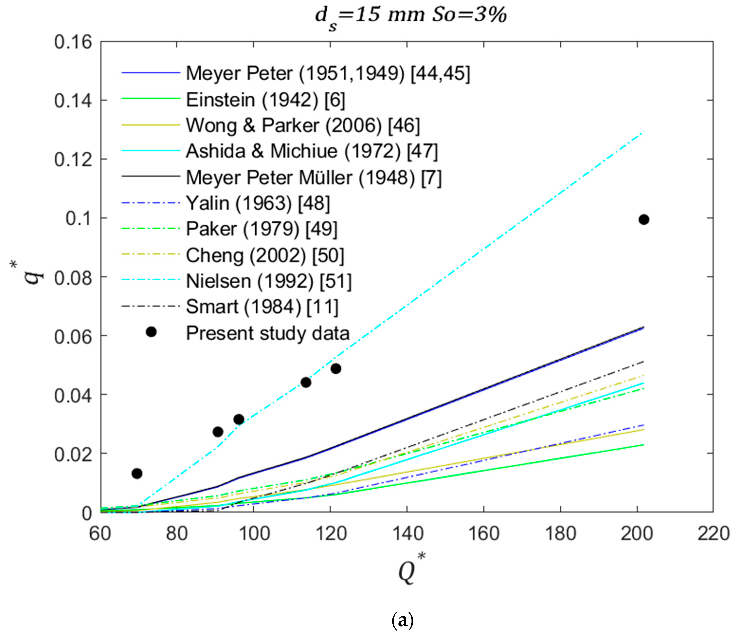
The results of this experimental model were compared with equations obtained for gravel bed rivers in previous studies (presented in
Table 1). The comparison between the different equations and Equation (12) states the following. For uniform diameters (10 mm, 15 mm and 25 mm) and for the smallest slopes analyzed (3% and 3.5%) the experimental transport rates show similarity to those obtained with the Nielsen simplified [
51] equation (
Figure 4a,
Figure 5a and
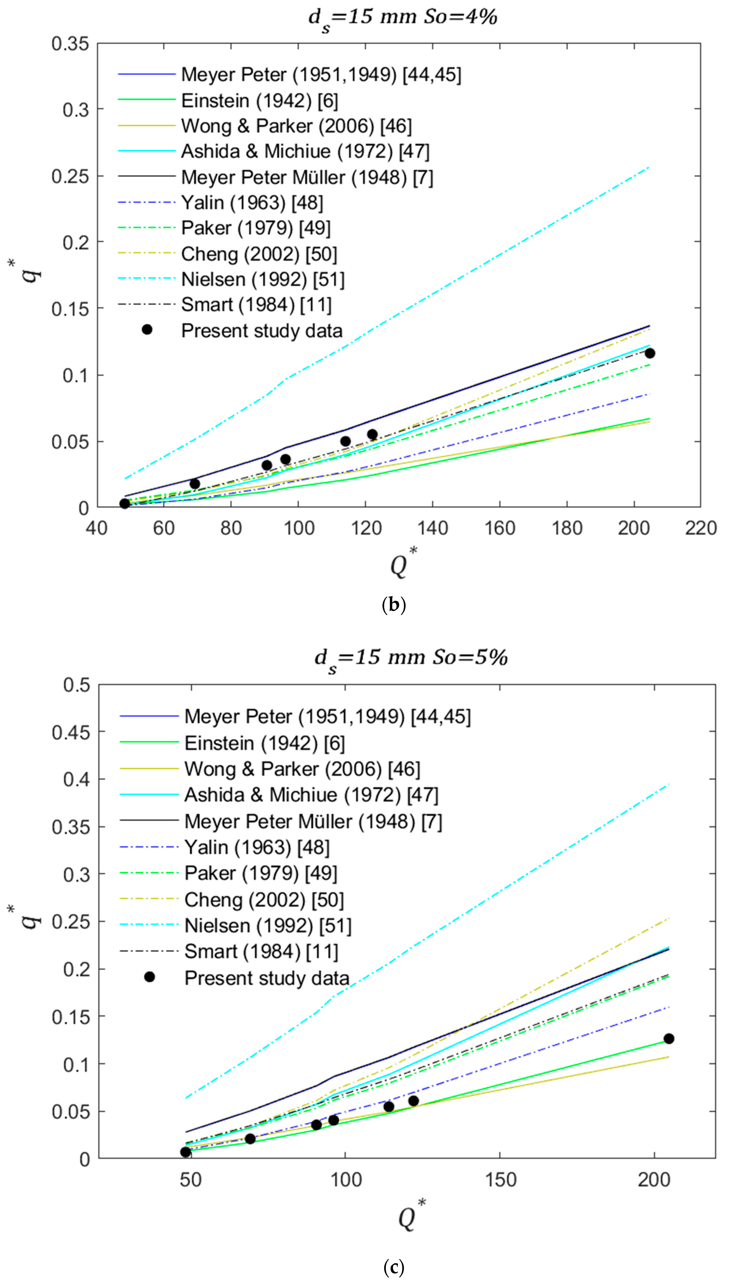
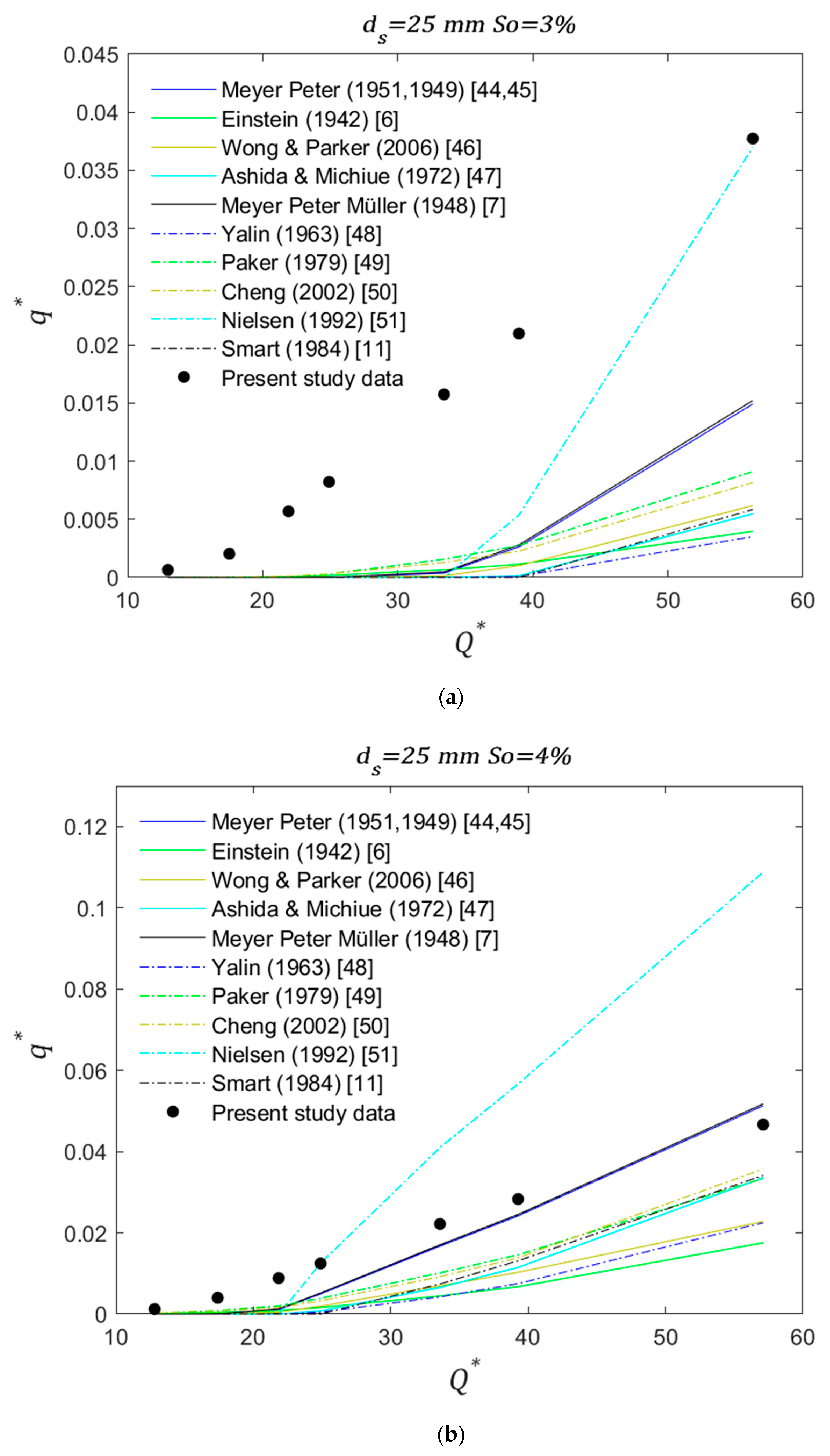
Figure 6a). However, as diameter size increases this similarity starts to decrease. Additionally, with a few exceptions, the laboratory rates tend to be higher than all the values from the equations in the literature. As slope increases to intermediate (4% and 4.5%), the experimental rates start to decrease with respect to the calculated rates and became similar to [
11,
47,
49] for
ds = 10 mm and 15 mm (
Figure 4b and
Figure 5b, respectively), and to [
7,
44,
45] for
ds = 25 mm (
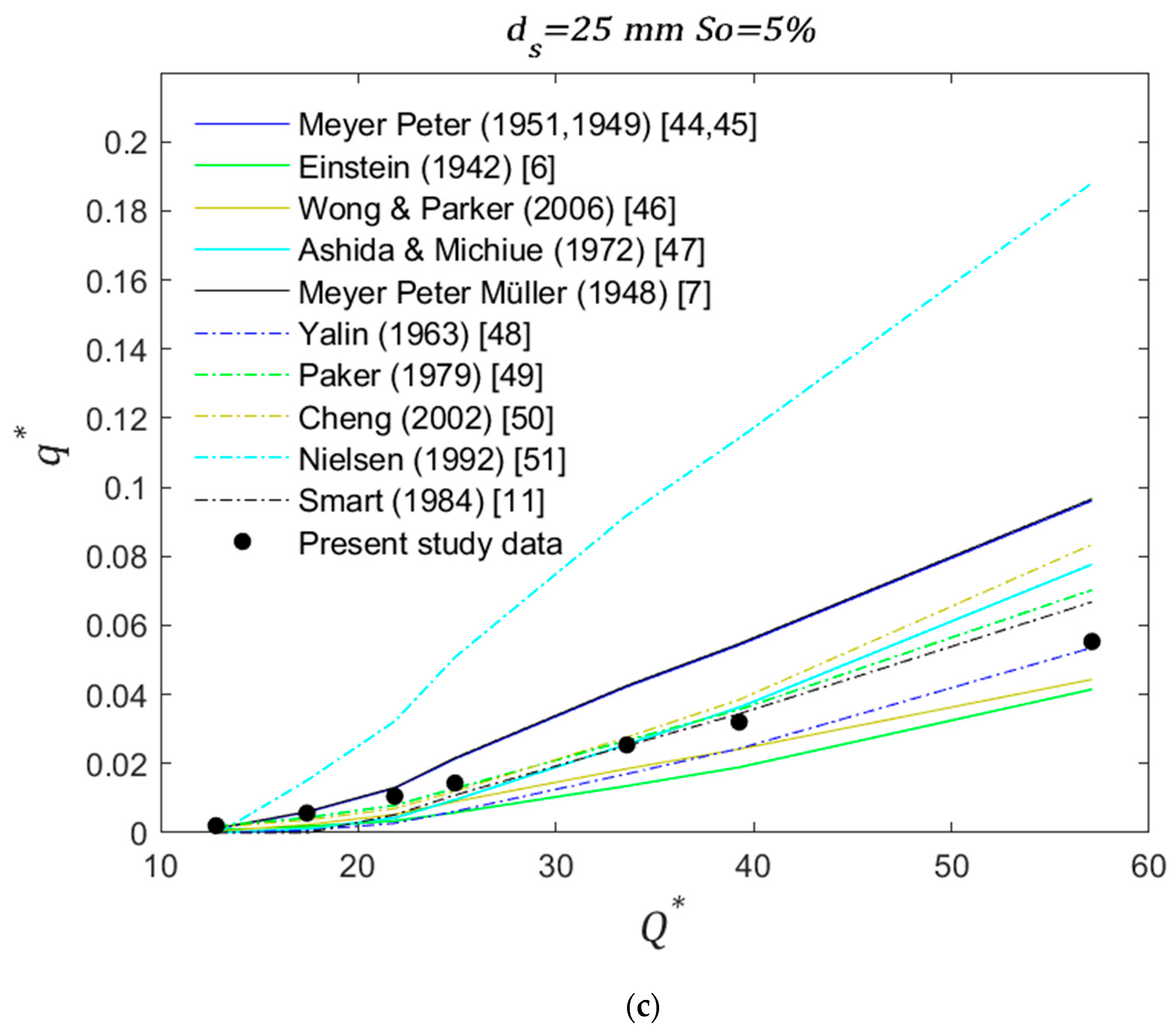
Figure 6b). For the highest slope (5%) experimental rates are similar to [
6,
46] for
ds = 10 mm and 15 mm (
Figure 4c and
Figure 5c, respectively), [
48] for
ds = 15 mm (
Figure 5c), and [
11,
48,
49] for
ds = 25 mm (
Figure 6c).
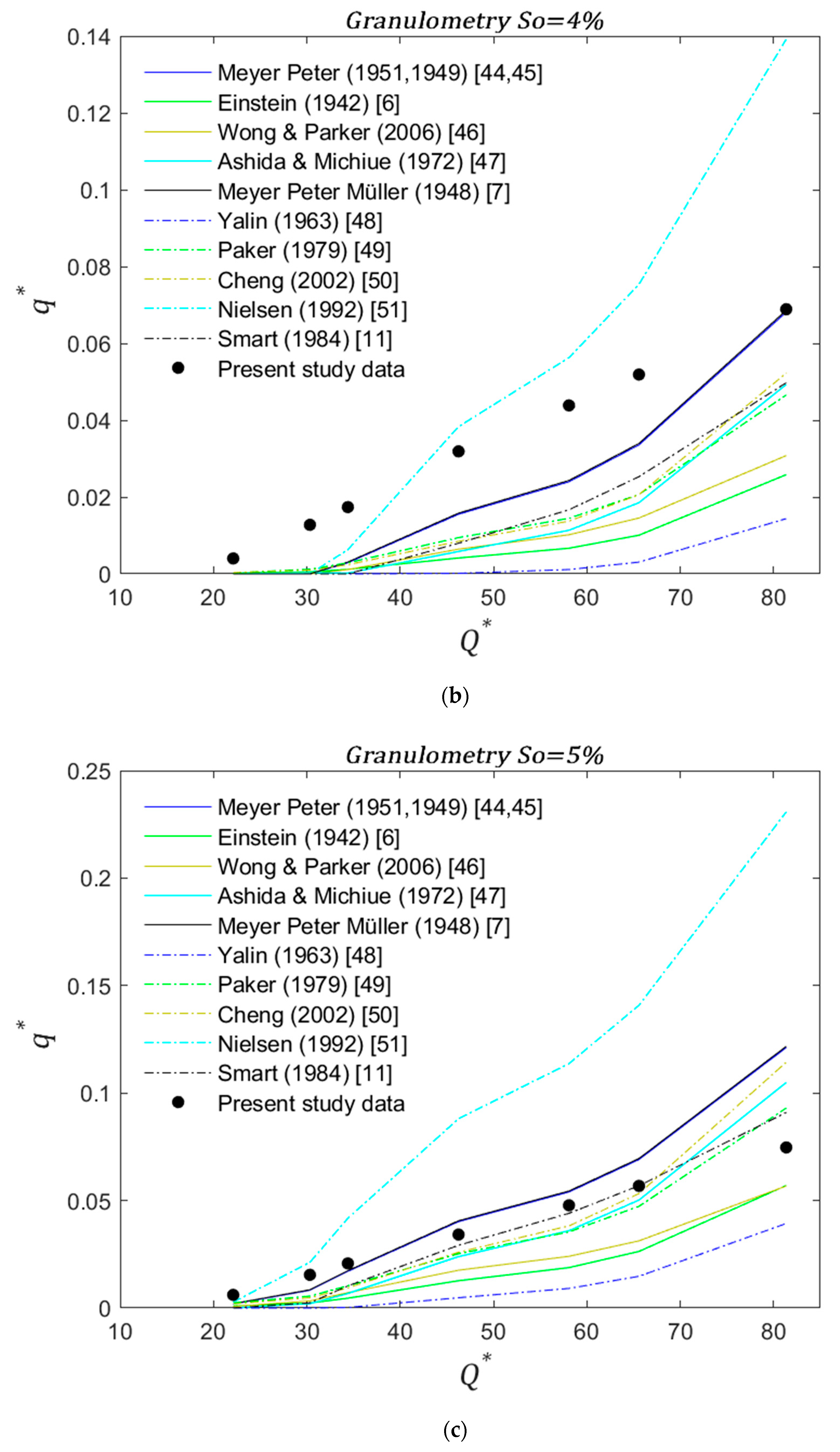
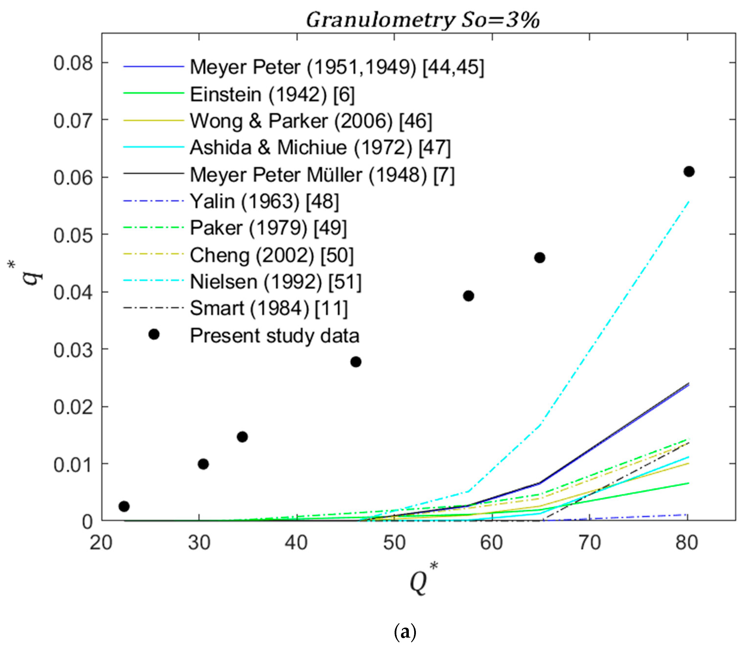
For grain size distribution in Case D, the equations overestimate the measured rates for slopes of 3% (
Figure 7a). For intermediate slopes (4%), slight similarities are reported with [
7,
44,
45,
51] (
Figure 7b). For the highest slopes (5%) experimental rates are similar to [
11,
47,
49,
50] (
Figure 7c). As observed from the comparison, some similarities are observed between previous models and Equation (12). Since most of the models do not report a range of slopes, special attention is placed on the model in [
11] given that this model was developed considering high slopes (up to 20%). The experimental transport rates show considerable agreement with this model’s rates, especially for slopes of 4% and 5%. Since the model has been demonstrated to perform well for steep slopes [
20], it may be concluded that the experimental model developed here could be used to estimate bedload transport rates in streams with slopes of up to 5%.
For all the cases simulated (Case A, B, C and D), the highest dimensional rates were reported for Case A (10 mm), then Case D (grain size distribution), then Case B (15 mm), and the smallest rates correspond to Case C (25 mm). For the same slope and discharge, larger particle diameters produced smaller transport rates. Though the grain size distribution contains the smallest diameter, it also has larger particles that allow an arrangement of particles which increases the resistance to movement that the flow must overcome to transport sediment. Additionally, the presence of larger particles absorbs part of the shear stress that can move sediment.
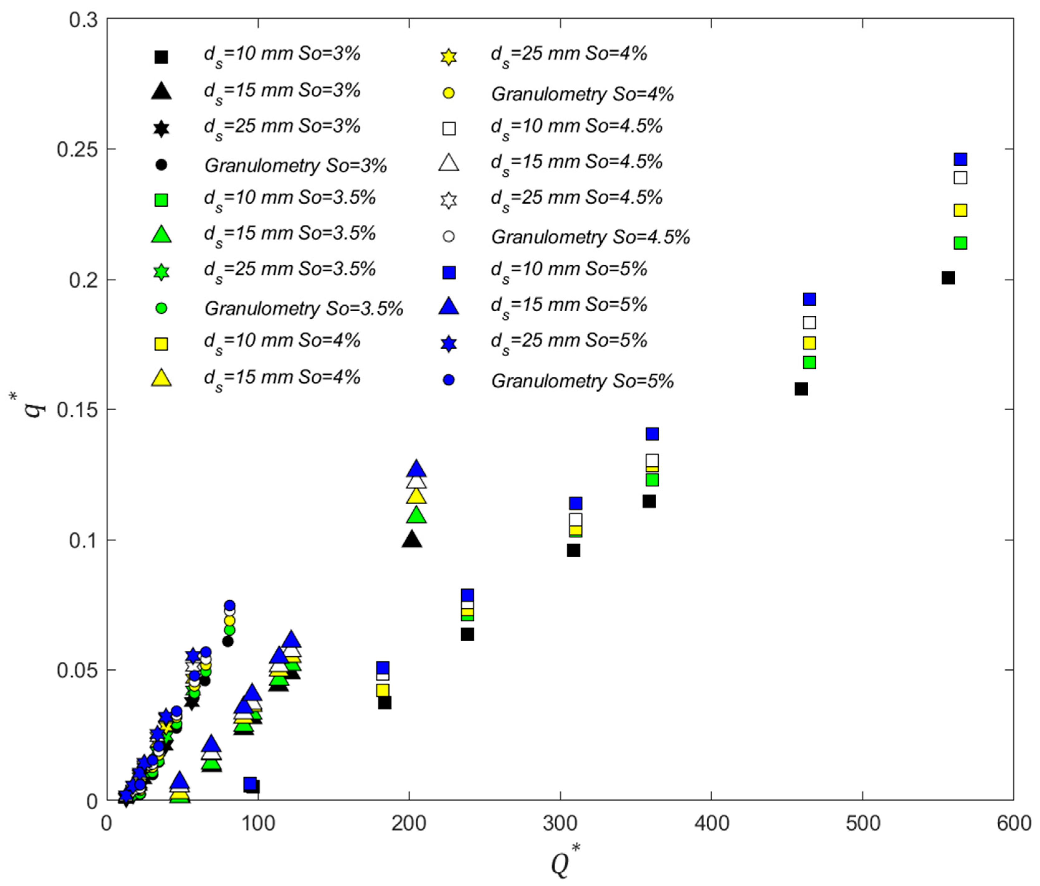
Considering just the results of the present study, for mild slopes the difference between the bedload transport rates obtained for the four cases (A, B, C and D) is higher than for the high slopes. With a slope of 5% the difference between highest and lowest transport rate (for the same discharge) has a value of 12% approximately. For 3% the difference is 35%, indicating that as slope increases particle diameter distribution decreases its impact on transport rate. Additionally, as can be observed in
Figure 8 that presents the transport rates obtained from the experiments, dimensionless transport rates for Case C (
ds = 25 mm) and Case D (Granulometry) have similar behavior. Since characteristic diameter
d84 (20.8 mm) was used to put variables in dimensionless form for Case D, this supports the definition of
d84 as the characteristic diameter for sediment mixtures [
54,
55,
56]. Even though the grain size distribution is built from the same uniform diameters, this fact could lead to the idea that for steep slopes the size distribution may have less influence on the transport process, and can be represented with a single particle size [
54].
A comparison was performed between the estimations from the equation developed without considering the gravity vector projection and Equation (12) that does include the gravity correction. The data used for this comparison corresponds to the bedload transport measurements for Case A, Case B and Case C. This data was selected because the data used for Equation (12) is independent of these three sets of data. In
Figure 9 the results of the comparison are presented. As can be observed, considerable improvement of the prediction capacity is achieved when gravity vector projection is considered. The predicted bedload transport rates without correcting the gravity vector are out of the range of an order of accuracy. These predictions overestimate the measured values by 1.5 orders of magnitude. Therefore, the correction of the gravity vector to account for the variation produced by steep slopes improves prediction capacity of the bedload transport models as demonstrated by [
20].
Considering the level of agreement between bedload transport rates’ formulae and field and laboratory measurements reported in several studies that can reach differences as high as eight orders of magnitudes [
16], predictions within an order of magnitude could be considered satisfactory. The range
0.1 < q*calculated/q*measured <10 represents the range within an order of accuracy, and it has been defined as the reference to consider bedload predictions valid [
55,
57,
58]. Even though bedload sediment transport has been studied for several decades, higher accuracy has not been possible to obtain due to factors such as the highly fluctuating nature of sediment transport, together with the fact that its predictions are based on average flow conditions [
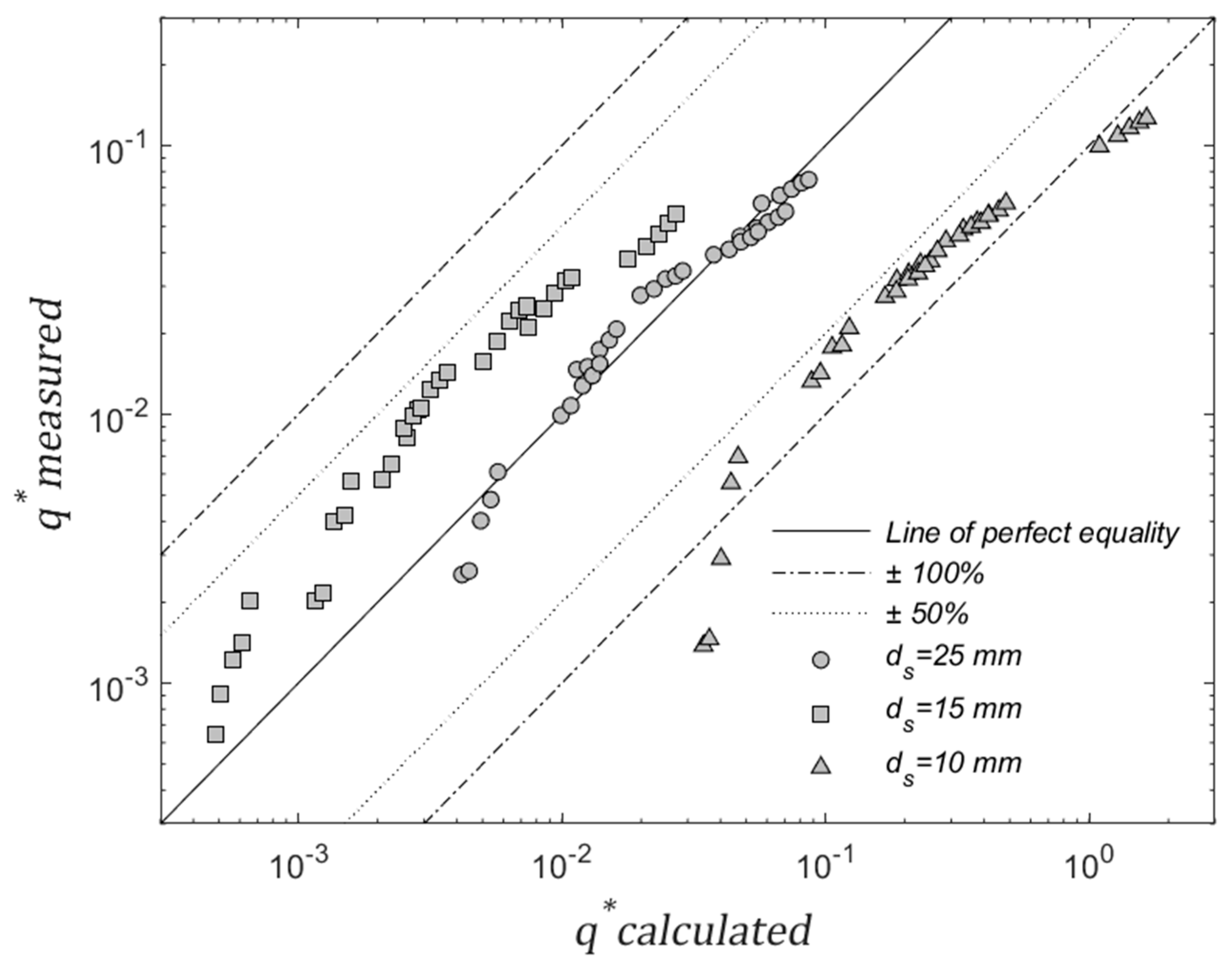
3]. To determine the prediction capacity of Equation (12), predictions are compared with the measured transport rates obtained for Case A, Case B, and Case C considering that this data is independent from the data used to obtain Equation (12) (Case D). This set of data had to be selected due to a lack of data with the level of detail required for calculations of the transport rates with Equation (12). In
Figure 10. measured and calculated transport rates are presented. The line of perfect equality and the lines defining the range
0.1 < q*calculated/q*measured<10 are also presented. As observed, eight points of the 105 considered do not meet this validation criteria. This represents that 92% of the data fall within the range of an order of magnitude. Since verified predictions correspond to uniform shape material and size and the model was obtained with a size granulometric distribution and uniform shape, we may assume that this methodology could be verified for laboratory simplified environments (uniform sediment size and shape). Therefore, it can be used to reduce the level of simplification and thus obtain a model that can be applicable to field conditions. The consideration more general conditions, especially for sediment such as that with larger, almost immobile, sediment particles and natural forms, can lead to the improvement of the prediction capacity of a model obtained based on the methodology applied here.
6. Conclusions
Equations have been proposed to determine bedload sediment transport rates. Early developments mostly considered mild slopes and fine sediment particles. More recent studies have focused on the study of bedload transport of gravel bed rivers, but only few have considered steep slopes. The present study aims to validate the experimental procedure to address the determination of bedload transport rates in steep channels with coarse material in laboratory environments. As a result, a simplified model is proposed to estimate bedload transport rates based on easily measured primary variables. Not all flow and geometry parameters involved in the bedload transport process are feasible for inclusion in the analysis. Therefore, in this study the most representative parameters were established based on their individual correlation with sediment transport. These parameters are dimensionless forms of discharge, flow depth, and slope. The parameters were used to obtain a mathematical model based on the experimental results. Case D that used a grain size distribution similar to a gravel bed river was selected as the most representative of the cases simulated. An improvement to previous models for bedload transport rate is the direct consideration of slope as an independent variable. Even though previous models include slope as part of other parameters such as shear stress, due to the impact that it has on transport rates in the proposed model it is considered as a primary variable.
The experimental model was compared with a range of widely used equations to determine sediment transport in gravel bed streams. The available models present a wide range of transport rate values for the same discharge. When reported, sediment diameters coincide with the diameters used here. However, it is important to note that the range of diameters simulated is narrower than those of the equations in the literature. Sediment shape and size were maintained constant for some of the equations in
Table 2, but natural sediment was also considered in some studies. As can be seen in
Figure 4,
Figure 5,
Figure 6 and
Figure 7, both slope (steep) and sediment size (coarse) play an important role in the transport process. Depending on the combination of these two parameters the simulated rates agree with some of the equations available in the literature for streams with particle sizes similar to those considered here. As stated, slope and sediment size have an important role in the final transport rates. To establish more concisely the reason for similarities or differences between equations, the variations of these parameters need to be considered. When compared with a model developed for steep slopes [
11], good agreement is reported for the experimental model especially for cases with the highest slopes (4–5%).
For the lower slopes, the behavior observed in the experimental simulations displays a considerable difference between experiments with uniform diameters and grain size distribution. This difference is reduced as slope increases. This finding leads to the conclusion that for high slopes the transport process can be estimated using a representative diameter. As in previous studies, the representative diameter d84 has been found to be appropriate. However, more data are needed to affirm this supposition because the grain size distribution used here was built with just three different particle diameters and they were the same as those used for the uniform size experiments.
The present study had the main objective of validating the laboratory methodology used to estimate bedload transport rates. As observed from previous studies for steep slopes, a correction to the gravity vector leads to an improvement in the prediction capacity of bedload transport models. For the data in the present study, the improvement represents an order of magnitude. The predictions with corrected gravity mainly fall within an order or magnitude. When gravity is not corrected the error reported is 1.5 orders of magnitude. Additionally, the experimental model predictions were compared with a set of measured bedload transport rates. For this comparison, the prediction capacity of Equation (12) falls within an order of magnitude for particles of uniform shape (spheres). Therefore, this methodology has been verified for simplified laboratory simulations (sediment of uniform shape and size). Experimentation of more general scenarios such as irregular river geometry, non-uniform form sediment particles, and a more general granulometric distribution can be performed using this experimental methodology together with a verification with independent filed measurements to obtain a more applicable verified model.


 ,
, 


