Abstract
Drought is a fundamental physical feature of the climate pattern worldwide. Over the past few decades, a natural disaster has accelerated its occurrence, which has significantly impacted agricultural systems, economies, environments, water resources, and supplies. Therefore, it is essential to develop new techniques that enable comprehensive determination and observations of droughts over large areas with satisfactory spatial and temporal resolution. This study modeled a new drought index called the Combined Terrestrial Evapotranspiration Index (CTEI), developed in the Ganga river basin. For this, five Machine Learning (ML) techniques, derived from artificial intelligence theories, were applied: the Support Vector Machine (SVM) algorithm, decision trees, Matern 5/2 Gaussian process regression, boosted trees, and bagged trees. These techniques were driven by twelve different models generated from input combinations of satellite data and hydrometeorological parameters. The results indicated that the eighth model performed best and was superior among all the models, with the SVM algorithm resulting in an R2 value of 0.82 and the lowest errors in terms of the Root Mean Squared Error (RMSE) (0.33) and Mean Absolute Error (MAE) (0.20), followed by the Matern 5/2 Gaussian model with an R2 value of 0.75 and RMSE and MAE of 0.39 and 0.21 mm/day, respectively. Moreover, among all the five methods, the SVM and Matern 5/2 Gaussian methods were the best-performing ML algorithms in our study of CTEI predictions for the Ganga basin.
1. Introduction
Drought refers to an extended water shortage period. In terms of water resource imbalance or excess evapotranspiration and moisture deficiency, the adverse impacts can be magnified due to extreme event dry conditions [1,2,3,4,5]. Moreover, drought can result in enormous socioeconomic, agricultural, hydrological, and meteorological effects [6,7]. Climate change has increased the severity, frequency, and extent of droughts worldwide in the last decades [8,9]. Due to the direct relationship between drought and water availability, any changes in drought characteristics due to climate change impact water shortages and food security [10,11].
More than 150 indices have been developed for drought assessment, classification, and monitoring [12]. These include the Palmer Drought Severity Index (PDSI) [13]; the Standardized Precipitation Index (SPI) [14]; the Standardized Precipitation Evapotranspiration Index (SPEI) [15,16]; the Rainfall Anomaly Index (RAI) [17]; the Precipitation Evapotranspiration Difference Condition Index (PEDCI) [18], the Reconnaissance Drought Index (RDI) [19,20]; and many others, as can be found in the review by Mishra and Singh [21]. Among these indices, the SPEI is a widely used index for tracking drought evolution at different time scales of interest (i.e., 1, 3, 6, 9, 12, and 24 months) [15]. Scientifically, the SPEI was developed from the SPI but involved the reference evapotranspiration (ETo) and thus significantly exhibits the influential role of temperature in drought evolution side by side with rainfall deficit [22,23]. This study modeled a new drought index called the Combined Terrestrial Evapotranspiration Index (CTEI) in the Ganga river basin. It was developed for the assessment of drought characterization in the Indus, Ganga, and Brahmaputra river basins by utilizing hydro-metrological variables, i.e., precipitation (P) and potential evapotranspiration (PET), as well as gravity data, i.e., Gravity Recovery and Climate Experiment (GRACE) terrestrial water storage anomalies (TWSAs) [24]. Therefore, this study focused on estimating and modeling the CTEI based on machine learning models to evaluate the drought over the Ganga basin.
Prediction of droughts has continued to challenge climate and hydrology research because of the spatiotemporal scales’ complexity [25]. Statistical, dynamical, and hybrid models are applied in predicting droughts [26,27,28]. With the development of computer technology, machine learning (ML) models have been applied in hydrological research to reveal complex hydrological phenomena [29,30,31], including in predicting droughts [32,33,34]. Several ML algorithms, such as support vector machines (SVMs) [35,36], artificial neural network (ANN) models [37,38], radial basis function (RBF) neural networks [39], fuzzy logic models [40], and extreme learning machines (ELMs), have been used in hydrological research [41]. For example, ANNs and SVMs are the most commonly applied techniques in developing drought prediction models [42,43,44,45]. The SVM, ANN, and k-nearest neighbor (KNN) techniques have been applied to predict drought in Pakistan [8]. The SVM and KNN algorithms have been applied to predict the PDSI over 116 years in Turkey [46]. Khan et al. [6] developed drought prediction models for Pakistan by applying the SVM, ANN, and KNN techniques.
Moreover, it has been reported that the accuracy of the SVM technique was higher than that of the ANN algorithm in predicting the SPI for Iran [47]. Most artificial intelligence models are highly accurate, although they are complex and have high computational costs during the training stage. In contrast, rule-based decision trees (DTs) and tree-based ensemble methods, e.g., gradient boosting (GB) and random forest (RF) methods, have lately become attractive because they are simple and at the same time still powerful and robust predictive algorithms [48,49]. Hassan et al. [48] predicted global solar radiation by applying bagging, GB, RF, and DT methods and comparing them with multilayer perceptron (MLP) and support vector regression (SVR). It was reported that the accuracy of tree-based models was the best. Recently, a novel, simple tree-based ensemble method named XG-Boost has been developed; it is an improved version of gradient boosting with higher computation efficiency and better capability to deal with overfitting problems [30]. Based on the techniques mentioned above, 12 different data-driven models were investigated to forecast the CTEI in this study. Machine learning models differ in terms of their input parameters. Five variants of each model were built, changing the applied machine learning algorithm for each: RF, SVM, boosted trees, bagging, and Matern 5/2 Gaussian process regression (GPR). These algorithms were applied due to their high performances in previous studies. They are very good at learning complex and highly nonlinear relationships. Therefore, the objectives of this study are to (1) fit five machine learning algorithms for the modeling of the CTEI prediction based on advanced models derived from artificial intelligence theories; (2) compare the accuracy and stability of these models, and (3) determine which were the best outcomes provided by the five models based on the prediction accuracy with the best combination of the input variables.
2. Materials and Methods
2.1. Study Area
The Ganga river basin (GRB) is one of the most populous (about 440 million people) river systems in the world [10]. The basin is situated in the northern part of the country. It lies between latitudes 21°32′8.6′′–31°27′36.2′′ N and longitudes 73°14′33.4′′–90°53′18.9′′ E, covering an area of 1,086,000 km2 (Figure 1).
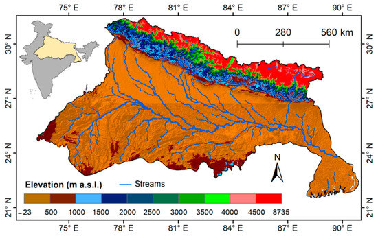
Figure 1.
The Ganga river basin’s elevation map and its tributaries along with a scale of the varying elevation.
The GRB spreads out into four countries, India (79%), Nepal (14%), Bangladesh (4%), and China (3%). In India, it covers 861,452 km2, which is nearly 26% of the country’s total geographic area [50]. The GRB originates in the Himalayan Mountains at the Gangotri glacier’s snout, at an elevation of ~7000 m a.s.l. The Bhagirathi and Alaknanda Rivers’ confluence occurs in Devprayag, which is then officially called the Ganga River. The Ganga River’s main tributaries are the Yamuna, the Ramganga, the Gomti, the Ghaghra, the Sone, the Gandak, the Kosi, and the Mahananda. It flows for about 2510 km, generally southeastward, through a vast plain to the Bay of Bengal. The primary source of water in the Ganga River is surface runoff generated by precipitation (~66%), base flow (~14%), glacier melt (~11.5%), and snowmelt (~8.5%). The GRB receives 84% of total rainfall during the monsoon season (June to October). The monsoon season accounts for 75% of the rain in the upper basin and 85% of the rain in the lower basin [51]. The elevation range across the basin varies from sea level to the highest mountain peak (~8850 m a.s.l). Several researchers have documented drought years in the region. For example, the NRAA [52] reported that India had experienced 22 large scale droughts years—in 1891, 1896, 1899, 1905, 1911, 1915, 1918, 1920, 1941, 1951, 1965, 1966, 1972, 1974, 1979, 1982, 1986, 1987, 1988, 1999, 2000, and 2002—and also that their frequency had increased during the periods 1891–1920, 1965–1990 and 1999–2002. Rathore et al. [53] reported that India experienced three major droughts in 2002, 2004, and 2009. A drought occurred in Tharparkar, in Sindh province, starting in 2013 and reaching its most devastating point between March and August 2014 [54]. Kothawale and Rajeevan [55] documented several rainfall deficit years between 1871 and 2016. They reported four deficit years (2004, 2009, 2014, and 2015) between 2003 and 2016.
2.2. Data Used
2.2.1. GRACE Terrestrial Water Storage Anomaly
In this study, 168 monthly GRACE data gravity solutions (level-3 RL-05, particular harmonics) at 1° × 1° spatial resolutions were acquired from three research agencies, the Center for Space Research (CSR) at the University of Austin/Texas, the NASA Jet Propulsion Laboratory (JPL), and the German Research Centre for Geosciences (GFZ), and were used to determine TWSA changes from January 2003 to December 2016 (14 years) (Table 1). However, 17 months’ worth of GRACE solutions were missing during the observation period; therefore, a particular month’s missing solution was replaced by the available sequent months (before and after) [56,57]. The GRACE TWSA data obtained from three data centers (JPL, GFZ, and CSR) were averaged to reduce the gravity field noise [58,59]. The TWSA includes the groundwater storage anomaly (GWSA), soil moisture storage anomaly (SMSA), canopy water storage anomaly (CWSA), surface water storage anomaly (SWSA), and snow water equivalent anomaly (SWEA), as expressed by Equation (1).

Table 1.
Detailed descriptions of each dataset used in this study.
2.2.2. Global Land Data Assimilation System (GLDAS) Observation
Global Land Data Assimilation System (GLDAS) is a joint project designed by NASA, the National Oceanic and Atmospheric Administration (NOAA), and the National Centers for Environmental Prediction (NCEP) by integrating the hydrological components obtained from ground and satellite-based observations with satisfactory spatial and temporal resolutions [60]. The details of the data products are described by Han et al. [61]. The GLDAS data comprises data for four land surface models (LSMs): the community land model (CLM2.0) [62], variable infiltration capacity (VIC) [63], National Oceanic and Atmospheric Administration (NOAH) [64], and Mosaic [65]. The spatial resolution of all the LSM data is about 1° × 1°. For monthly Total Water Storage (TWS) data obtained through GLDAS, a summation of the monthly soil moisture (SM) layer, snow water equivalent (SWE), and canopy water storage (CWS) from 2003 to 2016 from four LSM datasets were used (Table 1). The average of four LSM datasets was used to estimate the monthly TWS with minimum bias [66]. None of these LSM datasets includes groundwater storage or surface water storage (SWS) [60,62]. We assumed that the SWS in the study area was likely to be a minor component or a small contribution over the region; therefore, it was neglected. Numerous previous studies neglected the SWS changes for canopy water storage (CWS) estimation; for instance, Rodell et al. [60] and Tiwari et al. [67]. The GLDAS TWSA was converted into anomalies with the same considerations as GRACE data (i.e., the baseline period of January 2004 to December 2009). The GWSA was obtained by subtracting the model-based from the [68] by rearranging Equation (1), as is widely used in different regions of the world to isolate the GWSA from the GRACE-derived TWSA [60,67].
2.2.3. Tropical Rainfall Measuring Mission
The Tropical Rainfall Measuring Mission 3B43 Version 7 (TRMM-3B43-V7) monthly research precipitation data at 0.25° × 0.25° spatial resolutions were used for the Indus Ganga river basins during the period 2003–2016 [69] (Table 1). This product is commonly used worldwide for global precipitation analysis, for which its algorithm combines several instruments [69]. Nonetheless, several authors have compared the TRMM data with observational data and reported good accuracy [57,70,71].
2.2.4. Potential Evapotranspiration
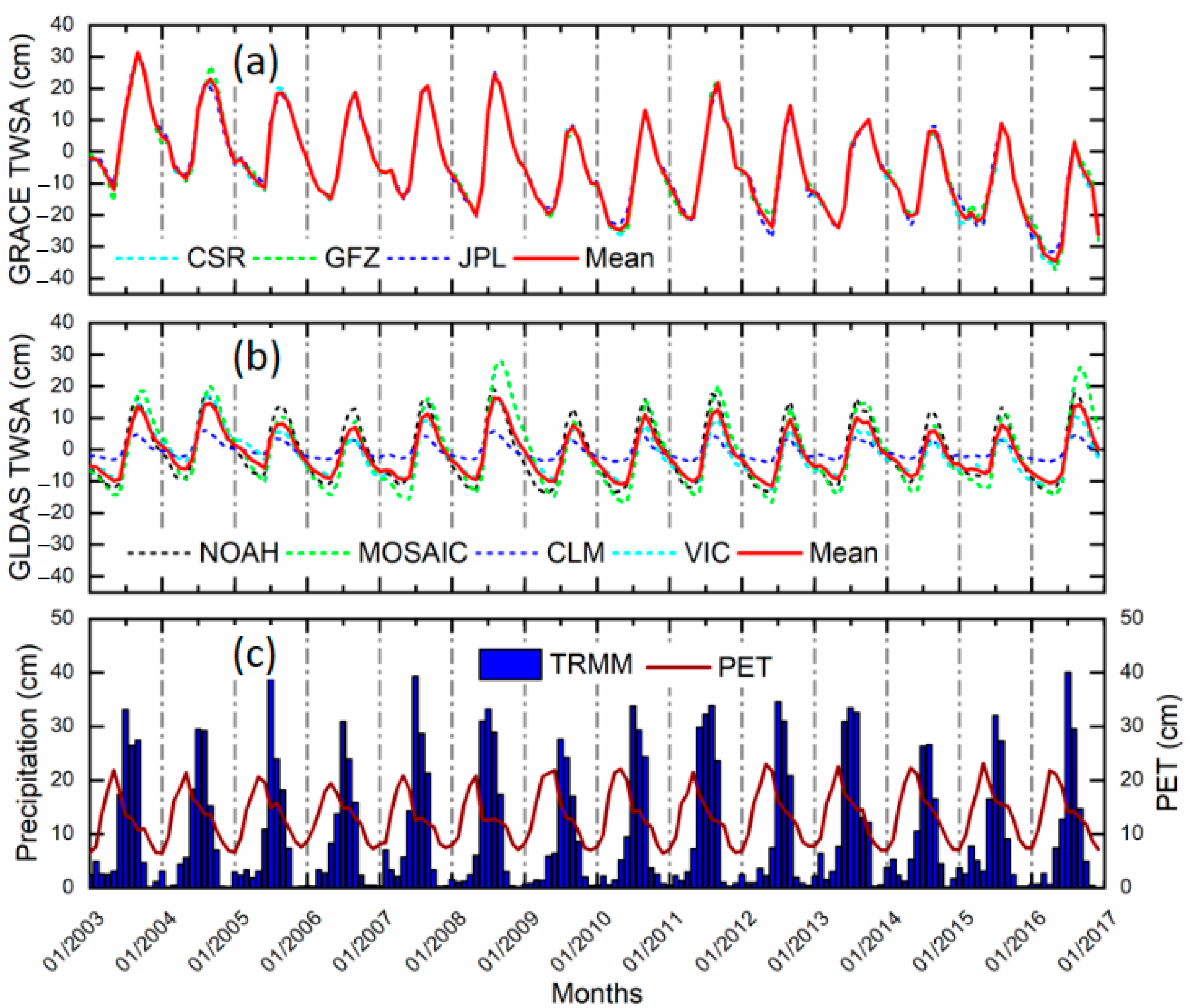
Datasets with a spatial resolution of 1° × 1° for the daily global potential evapotranspiration between 2003 and 2016 were used (Table 1). These data were generated from the climate parameter, i.e., extracted from the Global Data Assimilation System (GDAS) analysis fields. The NOAA generates the GDAS data every six hands it is freely available on the USGS website (https://earlywarning.usgs.gov/fews/product/81). The daily PET is calculated on a spatial basis using the Penman-Monteith equation [72]. The monthly and yearly PET was obtained using the accumulation of daily data. The monthly time series of GRACE terrestrial water storage anomalies, GLDAS observations, precipitation, and potential evapotranspiration are shown in Figure 2.
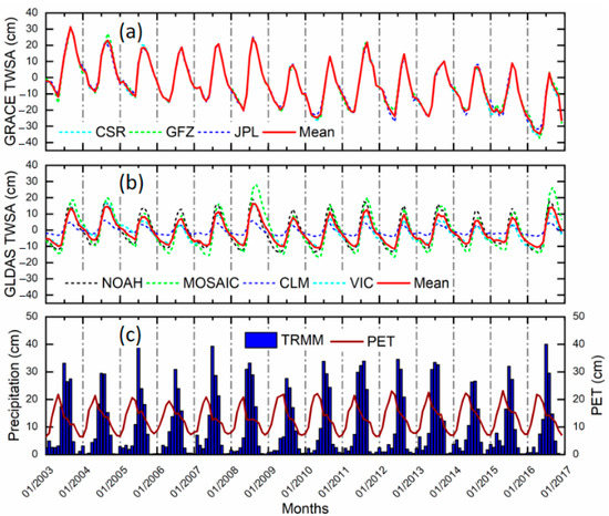
Figure 2.
Mean monthly values of (a) GRACE terrestrial water storage anomaly (TWSA) data (derived from three agencies), (b) GLDAS data (derived from four models), and (c) Tropical Rainfall Measuring Mission (TRMM) and potential evapotranspiration (PET) precipitation data averaged for the basin for the period from 2003 to 2016.
2.3. Methodology
2.3.1. CTEI Description and Calculation
The CTEI was derived using the GRACE TWSA data and meteorological variables (i.e., precipitation and evapotranspiration) for 2003–2016. This index was developed by Dharpure et al. [24] using hydrological and climatological conditions in the Indus, Ganga, and Brahmaputra river basins and which also highlighted that the CTEI was positively correlated with the ground observation wells. They also revealed that this index could quantify drought and severity on spatial and temporal scales. This model presents a comprehensive picture for estimating drought events at a regional scale where ground observation is limited.
For the calculation of the CTEI, firstly, the difference between the P and PET was calculated for each month [15] using the following Equation (2):
where D indicates the difference for each month . After that, the difference anomaly (DA) was derived using the following Equation (3) [73]:
where indicates the average value, which is calculated for the period from January 2004 to December 2009. The monthly climatologies concerning the and TWSA were derived based on the GRACE deficit approach [74]. The climatology of each month, i.e., from January 2003 to December 2016, was computed by averaging the values of the and TWSA in the same months of the year (e.g., all Januaries in the 14-year record were averaged) [73,74]. This monthly climatology was used to remove the influence of seasonality [75]. The DA and TWSA time series’ monthly residuals were obtained by subtracting the climatologies from each month’s and TWSA data, respectively. The obtained residuals were added together to get the combined water storage anomaly (CWSA), indicating the net deviation in the volume of water storage based on seasonal variability. Finally, we normalized the CWSA by removing the mean and dividing by the standard deviation of each month [74], as in the following Equation (4):
where indicates the Combined Terrestrial Evapotranspiration Index. The CTEI was compared with the pre-existing drought indices, with good correlations with the GRACE Groundwater Drought Index (GGDI) (0.88), the Water Storage Deficit Index (WSDI) (0.96), the Combined Climatologic Deviation Index (CCDI) (0.97), and Standardized Precipitation Evapotranspiration Index (0.49) [22].
2.3.2. Machine Learning Models
Support Vector Machine
A support vector machine is a supervised learning algorithm. It can also be used as a regression model, maintaining all the main features that describe the algorithm (e.g., maximal margin). Support vector regression (SVR) uses a similar SVM theory for the classification method, with a few slight changes. The limit of tolerance is set in approximation to SVMs, for which the problem has already been formulated. The main aim is to minimize the error by individualizing the hyperplane, which increases the limit of tolerance because a part of the error is tolerated. The goal of SVM is to make the function (x) as flat as possible. Hence, given the linear function, we can minimize the process and constraints, as shown in Figure 3, where: w and b are the dot products in x; ℇ is the maximum deviation value from the observed target values; ξ, ξ* are slack variables, greater than or equal to zero; and C is a constant that affects both the function of flatness and tolerated variations. The SVM estimation function (F) in any given regression scenario can be defined as follows in Equation (5):
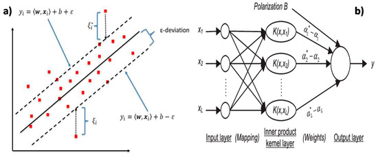
Figure 3.
(a) Example of support vector regression (SVR); errors do not matter as long as they are less than ε, while the deviations are penalized. (b) Typical architecture of an SVR algorithm.
W is the weightage vector; Tf represents the nonlinear transfer function, which projects the input vectors towards a very high dimension feature space; and b is the constant variable. The parameters used for the SVM algorithm were batch size = 100, C = 1, filter type = normalized training data, and kernel = poly kernel.
Decision Trees
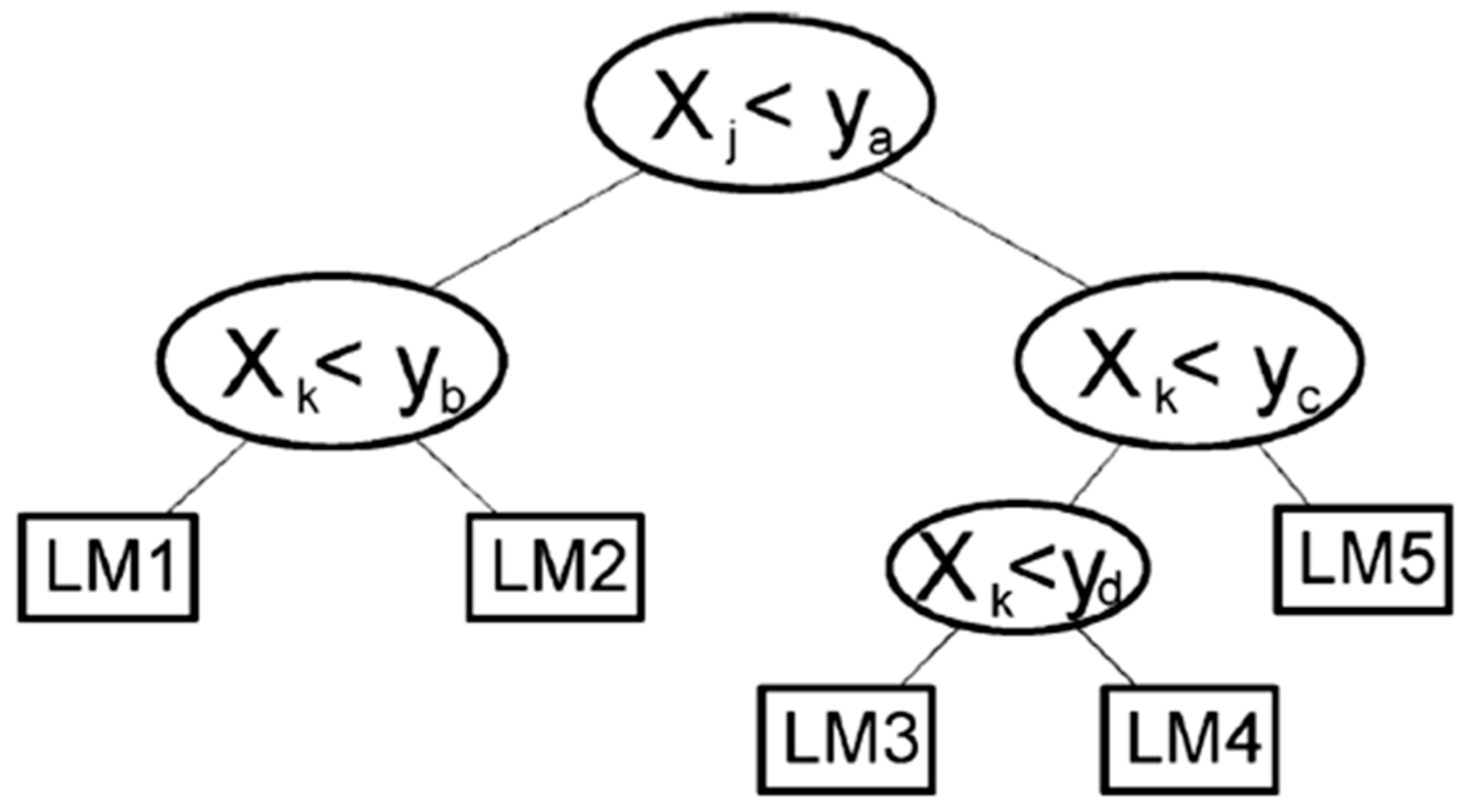
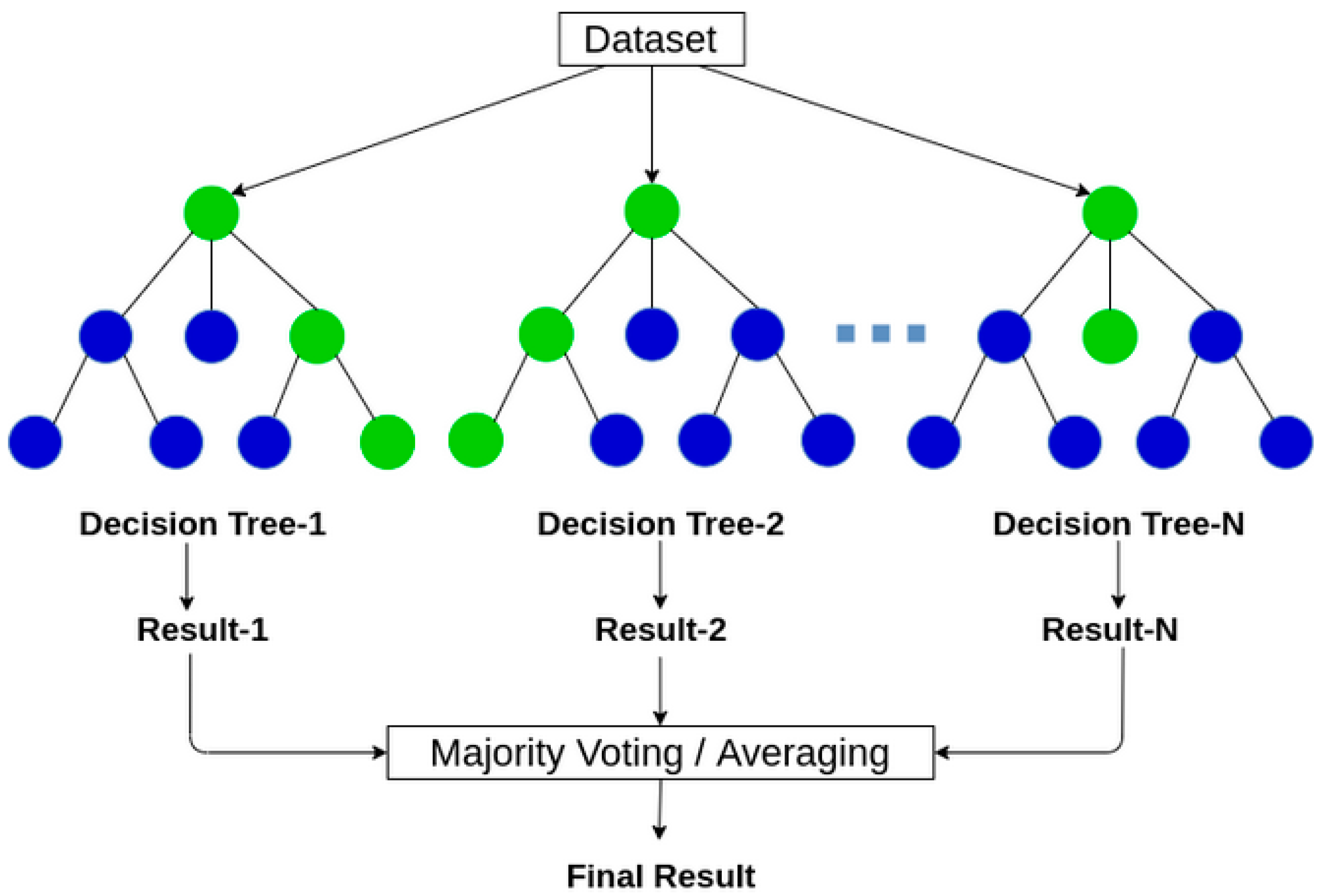
Decision-tree learning is a forecasting model for going from observations about a dot (represented in branches) to prediction and conclusions about the target value (represented in leaves). The primary aim is to create a model that forecasts the target value based on several independent inputs. An example is shown in the diagram on the right. Each internal node represents one of the input variables; there are edges to increase more children for each input variable. Each leaf has a value of the goal variable, given the input values of variables represented by the process from the root to leaf. In this study, various techniques were often deployed to construct more than one decision tree (Figure 4 and Figure 5).

Figure 4.
The typical architecture of a regression tree model; LM, linear model.
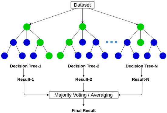
Figure 5.
Typical architectures of bagging or random forest models. The algorithms are different depending on the way the regression trees are built.
- Boosted Tree
Boosting is an ensemble technique to create a collection of predictors. In this technique, models are learned sequentially. Early learners fit simple models to the data and analyze data for errors. The boosted tree is performed based on an ensemble to train the new sample [76,77]. When a hypothesis misclassifies an input, its weight is increased. The next hypothesis is more likely to classify it correctly. Combining the whole set at the end converts weak learners into a better-performing model. A typical paradigm is Ada-Boost, which can be used for regression-type modeling; bootstrap-aggregated (or bagged) decision trees, an early ensemble method, construct numerous decision trees by frequently re-sampling training data using the replacement method and electing the trees for the consensus forecast; a random forest regression is a specified type of bootstrap assemblage.
- Bagged Tree
Bootstrap aggregation (bagging) is used when the goal is to reduce the variance of a decision tree. The bagging tree technique is a robust technique widely deployed in the accurate estimation of drought, which uses re-samples of the training datasets [78,79]. The first step involves bootstrapping the samples from the raw data that comprise the different training data sets. One of the bagging algorithm’s main advantages is that it combines all the trees to provide a combined tree model rather than a single tree model output. Also, it removes the instability that is present in the regression tree growth. This is done by removing the initial training datasets instead of novel training dataset sampling for each time step. The average of all the predictions from different trees is used, which is more robust than a single decision tree.
- Random Forest
An RF is simply a collection of decision trees whose results are aggregated into one final result [78]. Their ability to limit overfitting without substantially increasing error due to bias is why they are such powerful models. One way the random forests reduce variance is by training on different samples of the data. To increase the robustness of this model, a statistical inference technique called bootstrapping is used. Each of the trees which make up a particular forest is built up from random sub-sampling of datasets. This bootstrap method is based on a random draw with replacements. Hence, the term” random” is used in the name of this model. The final prediction of the model output is determined by an ensemble of methods from among all results from each tree making up the forest. This can be called the” majority vote.” One technique to avoid overfitting RF model application problems is to limit the minimum leaf size (min-leaf). This parameter determines the minimum number of observations used to create each child node; smaller mini-leaf values need a deeper learning process. The parameters used for each algorithm were bag size percentage = 100, batch size = 100, number of execution slots = 1, number of iterations = 100, and seed = 1.
At each step, the processing system divides the subdivision into two unconnected segments that decrease the value of the squared deviation, described as follows in Equation (6):
N (t) is the number of sample groups in connection (t), yi represents the value taken by target variables in the i unit, and ym equals the average of the target variable in connection t.
Matern 5/2 Gaussian Process
A Matern 5/2 Gaussian process regression is a random process. Any point x∈Rd is assigned a random variable f(x). The Matern 5/2 kernel takes actual data densities of the stationary kernel. It creates a Fourier transform of the radial basis function (RBF) kernel. It does not have any measure problems for high-dimensional spaces. The algorithm of the Matern 5/2 GPR is as follows in Equation (7)
P(f|X) = N(f|μ,K)
In Equation (6), f (x) = p (f(x1),...,f(xN)), μ = (m(x1),...,m(xN)), and Kij = κ(xi,xj). m is the mean function, and it is common to use m(x) = 0 as GPs are flexible enough to model the mean arbitrarily well. κ is a positive definite kernel function or covariance function. Thus, a Gaussian process is a distribution over functions whose shape is defined by K. If points xi and xj are considered similar by the kernel, the function values at these points, f(xi) and f(xj), can be expected to be similar too. All algorithms were implemented for -CTEI modeling using MATLAB (R 2019a) software. The CTEI datasets for all algorithms were divided into training sets for those from 2003 to 2013 and testing sets for those from 2014 to 2016.
2.4. Statistical Analysis
Actual data for the CTEI and modeled values were compared for the study period. To evaluate the accuracy of models, the following statistical indicators were selected: (1) root mean square error, (2) coefficient of determination, and (3) mean absolute error [80,81,82,83]. All parameters were defined as follows: is an observed or actual value,is a simulated or foreseen value,is the mean value of reference samples, and N is the total number of data points.
- Root Mean Square Error.
Root mean square error (RMSE) is a sample’s standard deviation about the differences between foreseen and actual values. It is given by Equation (8):
- 2.
- Coefficient of determination (Equation (9))
- 3.
- Mean absolute error (MAE)
The mean absolute error evaluates the mean magnitude of the errors in a set of forecasts without considering their sign. It is an average for the test sample of the absolute differences between foreseen and actual values. It is defined as follows in Equation (10):
3. Results and Discussion
3.1. Assessment of ML Models Performance
In this study, we developed twelve different data-driven models for predicting the CTEI in the Ganga basin. As discussed in the methodology, each of these models differed depending on the number and type of input parameters. We developed five variants corresponding to each of these models by changing the applied machine learning algorithm, namely RF, SVM, boosted trees, bagging, and Matern 5/2 GPR. The different input parameters used in the model building were the TWSA (from GRACE and GLDAS), evapotranspiration (ET), P, PET, wind speed (u), radiation, GWSA, air temperature (Ta), and surface temperature (Ts). These input parameters have also been used in previous studies [23,84]. The detailed setup combination for each model is given in Table 2.

Table 2.
The effectiveness of the considered models for the Combined Terrestrial Evapotranspiration Index (CTEI) estimate in the Ganga basin.
These models’ setups range from a simple model that depends on only important climatic variables, like evapotranspiration, to very complex models including complex climatic inputs and radiation and heat fluxes. Table 2 shows the implementation and effectiveness of all the twelve models in the CTEI estimates for the Ganga basin. Like those of model 7 and model 4, some of the model setups performed too poorly for all the five methods used. These models were the ones in which the following input parameters were used: PET, ET, radiation (R), net radiation (Rn), long-wave net radiation (LWN), and Ta. These models had R2 lower than 0.15 in all cases. The RMSEs and MAEs for all models were as high as 0.6, 80, and 65, respectively. Based on these statistical analyses, it can be observed that model 8 showed the best predictions for the CTEI when compared to the other model setups.
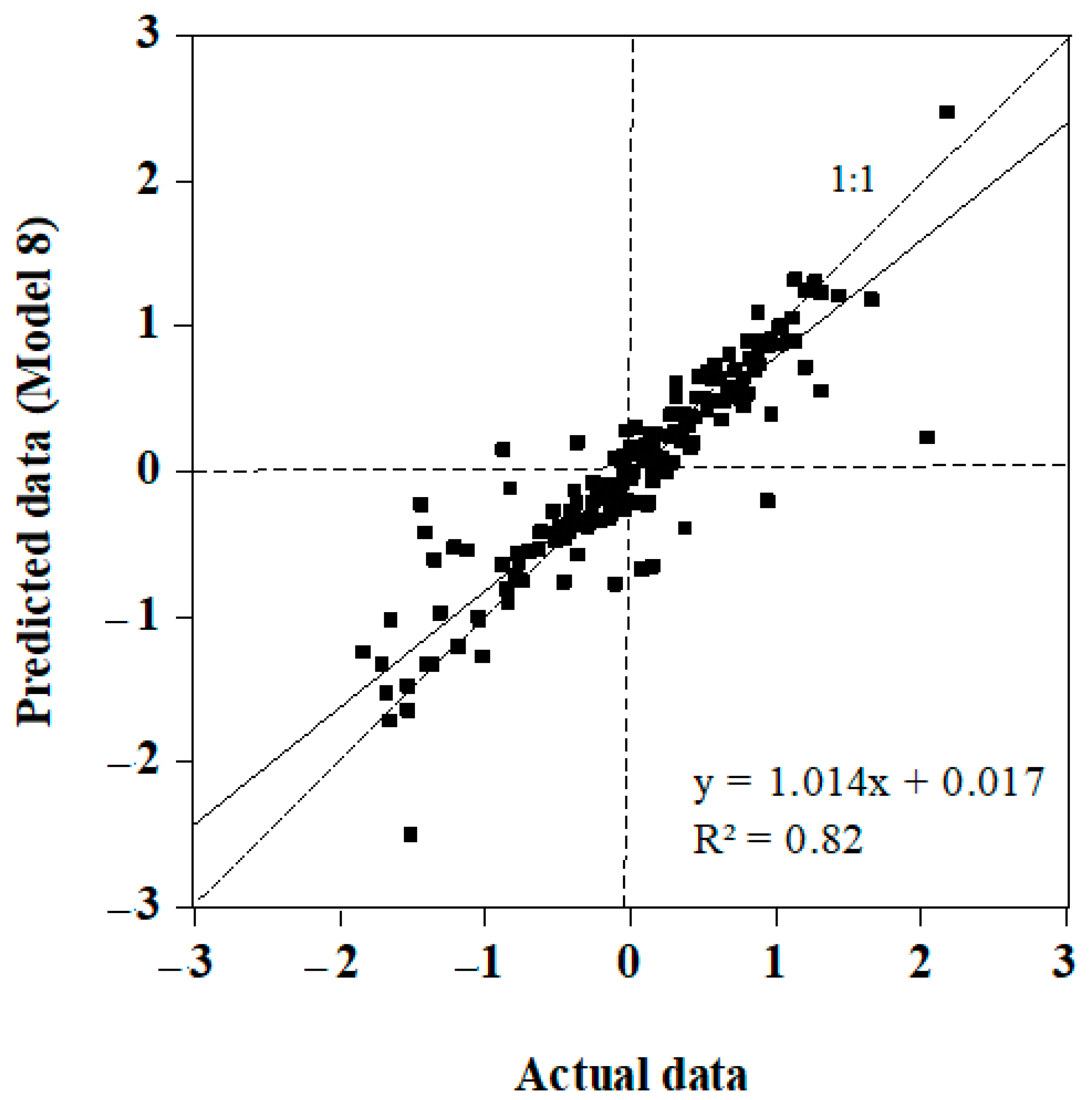
Moreover, among all the five methods used, the SVM and Matern 5/2 GPR methods were the most highly performing ML algorithms in our study of CTEI predictions in the Ganga basin (as detailed in Table 2). Model 8 showed the best performance among all the model settings. Most of the implemented ML algorithms used in model 8 showed higher values of R2 and the lowest values in terms of the RMSE and MAE. The SVM algorithm was characterized as the best performing method among all the five algorithms, with an R2 value of 0.82 (Figure 6) and the lowest errors in terms of the RMSE (0.33) and MAE (0.20).
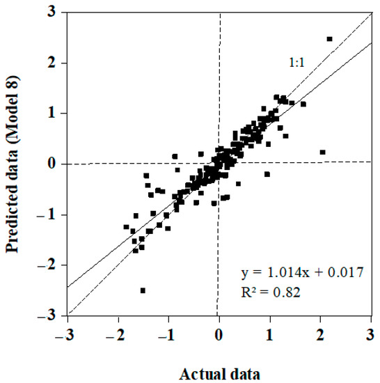
Figure 6.
The best model for predicting the CTEI with the implementation of the support vector machine (SVM) algorithm—model 8.
The residual plot for model 8 with the SVM method shows that the maximum errors in the CTEI predictions occurred in the range of 0 to 2 mm, as shown in Figure 7.
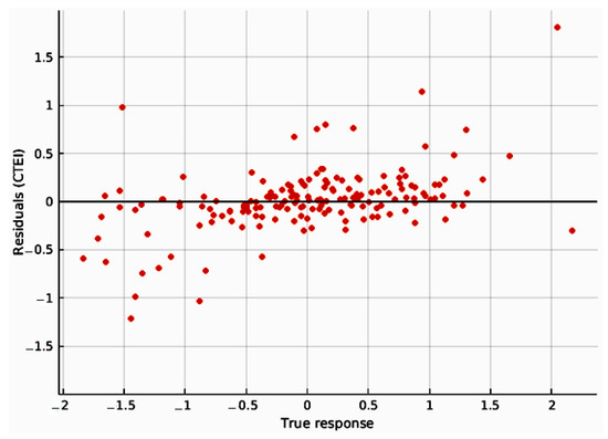
Figure 7.
The residuals versus the Ganga basin’s actual values for the best model (model 8 SVM).
Furthermore, the GPR boosted trees and bagged trees algorithms performed comparatively better, with R2 values of 0.75, 0.58, and 0.52, respectively. They also had very low values for the error statistics in terms of the RMSE (0.39, 0.51, and 0.58, respectively) and MAE (0.21, 0.34, and 0.38, respectively).
3.2. Comparison of Actual CTEI with Predicted CTEI
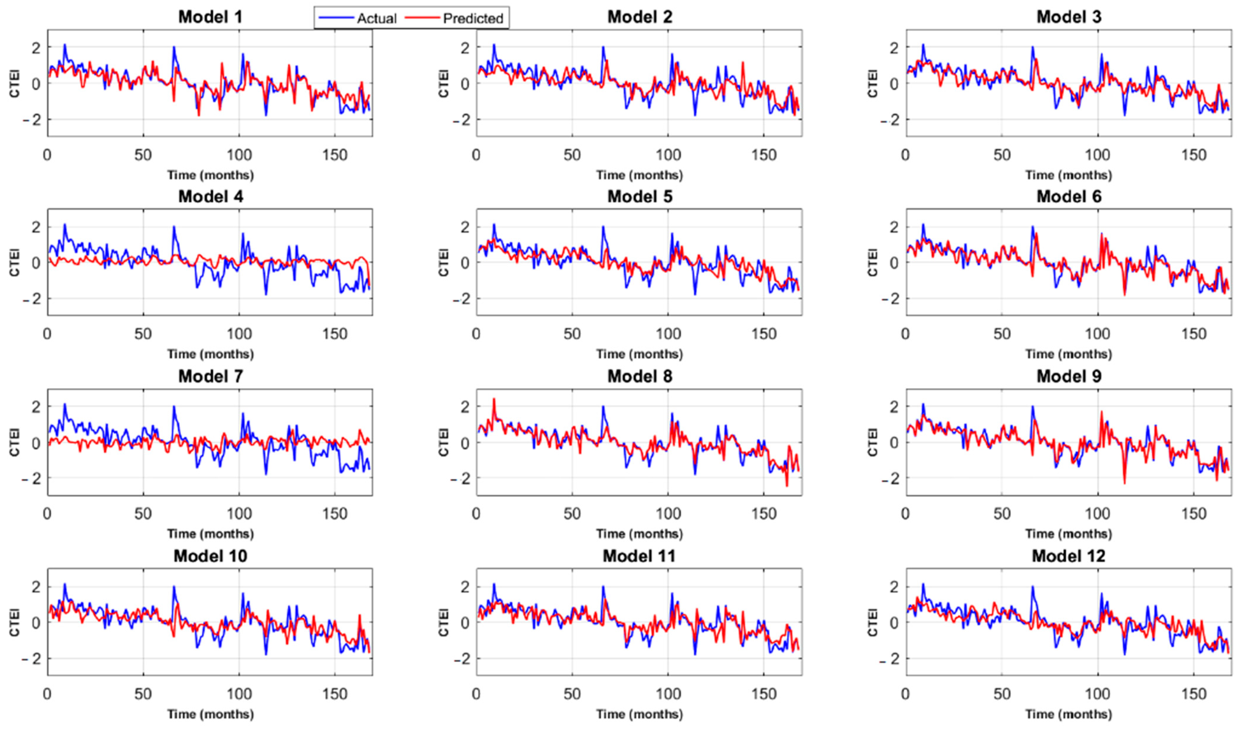
Figure 8 compares the actual CTEI with the predicted CTEI for all the twelve models, from which the best ML algorithm was obtained. It shows a plot for the years from 2003 to 2014. Models 4 and 7 performed the worst. The rest of the models performed comparatively well. As mentioned in the previous section, model 8 with the SVM algorithm provided the best CETI prediction compared with the observed CTEI. Table 3 shows the interannual variation for the observed and the predicted CTEIs for the years from 2003 to 2016.
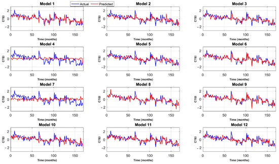
Figure 8.
Comparison of all the models with the best machine learning (ML) algorithm (model 8, SVM) for the actual and predicted CTEI values for 2003–2016.

Table 3.
Average actual and predicted CTEIs and differences and deviations for the best machine learning models in the training and testing periods in the Ganga basin.
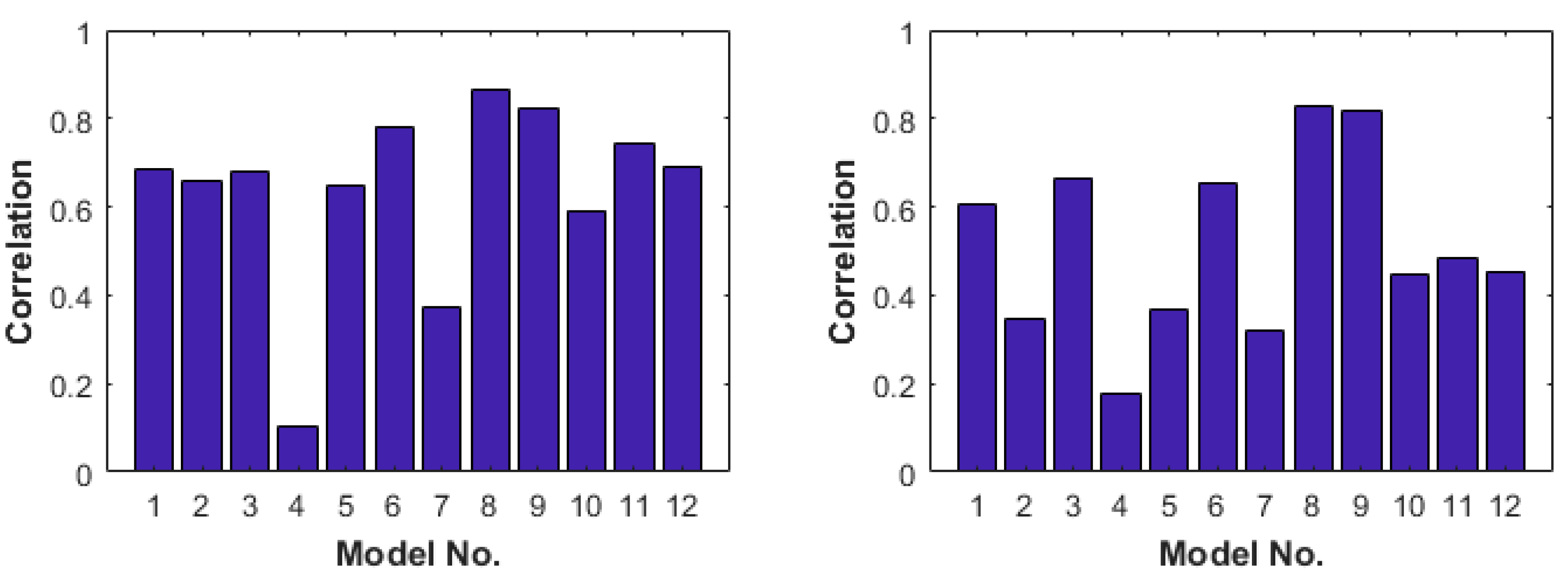
The maximum deviation in the CTEI predictions occurred in 2013, while the minimum deviation occurred in 2015, 10.31 and −0.02, respectively. Figure 9 compares the actual CTEI and predicted CTEI (model 8, SVM algorithm) for all the years. It can be observed that model 8 with the SVM algorithm could predict almost concurrently with the observed datasets, except for a few years. Figure 9 shows the correlation coefficients for both the training and testing periods of all the datasets using the best algorithm for each of the models. It can be observed that model 8 showed the highest correlation in the training and testing period, > 0.85. Model 9 also predicted the CTEI values equally compared to model 8, with correlations up to ~0.82 for both periods. As models and 7 performed too poorly, they showed the least correlation (<0.3) throughout the simulation period. The SVM algorithm worked best compared to all the other methods, and it has also been widely used previously [32,66,82].
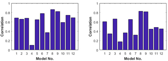
Figure 9.
The correlation coefficients of the predicted CTEI values from all the 12 models with the best-fitted algorithm (model 8 with the SVM algorithm) for the training (left side) and the testing period.
This study’s findings show that machine learning algorithms are one of the best, efficient, and most powerful tools that can be used for evapotranspiration prediction when there are limited datasets [23,45]. This indicates similarities to approaches with large-scale conceptual hydrological models [85,86]. It can be observed that when the models were given input variables like climatic parameters (P, Ta, Ts), sensible heat fluxes, as well as GRACE and GLDAS TWS datasets, the models resulted in highly accurate predictions [84,87]. Considering only the temperature and extraterrestrial radiation has advantages for ML algorithms [27,28,49].
These model predictions provide the CTEI based upon net evapotranspiration without intense data requirements [22,57]. These analyses show that when various variables, ranging from climate and radiation to heat fluxes—and further including GWSA, ET, R, , , SWN, LWN, P, and PET data-are used, a better opportunity is provided for predicting CTEI values with high accuracy. This is also supported by previous studies [10,24,29,34].
4. Conclusions
In this study, a new drought index called the CTEI was modeled based on five machine learning models (SVM, RF, boosted trees, bagged trees, and Matern 5/2 GPR). This index was driven by a combination of meteorological variables and the GRACE TWSA for the Ganga river basin. The monthly data were collected from 2003 to 2016 and divided into training (2003–2013) and testing (2014–2016) models. This research aimed to investigate the performances of the five selected machine learning models in predicting nonlinear interaction between limited input parameters to simulate the monthly values of the CTEI. Different combinations of satellite data with the hydroclimatic parameters, based on limited parameters (the ML models’ inputs), were used for CTEI estimation. After analyzing all the combinations, the main finding of this study was that the eight model settings (considering GWSA, ET, R, , , SWN, LWN, P, and PET) with the SVM algorithm showed the best performance among all the model settings in predicting the CTEI. This model also found the Matern GPR algorithm to be satisfactory. It achieved the second-highest rank for CTEI prediction. Model 6 ranked as the third-best option, achieving reasonable outcomes based on a data fusion of SWN, LWN, P, and PET.
Author Contributions
Conceptualization, A.E. and J.K.D.; methodology, A.E. and J.K.D.; software, A.E.; validation, A.E. and J.K.D.; formal analysis, A.E., J.K.D.; investigation, A.E., J.K.D., N.K., A.M., K.A., A.K.; writing—original draft preparation, A.E., J.K.D., N.K., A.M., K.A.; writing—review and editing, M.K., B.M., H.R.E., Y.B., A.R.M.T.I. and A.K.; visualization, A.E., J.K.D. and A.K.; supervision, A.E., J.K.D. and A.K.; project administration, A.K.; funding acquisition, A.K. All authors have read and agreed to the published version of the manuscript.
Funding
This research received no external funding.
Data Availability Statement
The datasets generated and/or analyzed during the current study are available from the corresponding author upon reasonable request.
Acknowledgments
This research did not receive any specific grant from funding agencies in the public, commercial, or not-for-profit sectors.
Conflicts of Interest
The authors declare that they have no conflicts of interest
References
- Akyuz, D.E.; Bayazit, M.; Onoz, B. Markov Chain Models for Hydrological Drought Characteristics. J. Hydrometeorol. 2012, 13, 298–309. [Google Scholar] [CrossRef]
- Mpelasoka, F.; Hennessy, K.; Jones, R.; Bates, B. Comparison of suitable drought indices for climate change impacts assessment over Australia towards resource management. Int. J. Climatol. J. R. Meteorol. Soc. 2008, 28, 1283–1292. [Google Scholar] [CrossRef]
- Paneque, P. Drought Management Strategies in Spain. Water 2015, 7, 6689–6701. [Google Scholar] [CrossRef]
- Maza, M.; Srivastava, A.; Bisht, D.S.; Raghuwanshi, N.S.; Bandyopadhyay, A.; Chatterjee, C.; Bhadra, A. Simulating hydrological response of a monsoon dominated reservoir catchment and command with heterogeneous cropping pattern using VIC model. J. Earth Syst. Sci. 2020, 129, 200. [Google Scholar] [CrossRef]
- Naumann, G.; Barbosa, P.; Garrote, L.; Iglesias, A.; Vogt, J. Exploring drought vulnerability in Africa: An indicator based analysis to be used in early warning systems. Hydrol. Earth Syst. Sci. 2014, 18, 1591–1604. [Google Scholar] [CrossRef]
- Khan, N.; Sachindra, D.A.; Shahid, S.; Ahmed, K.; Shiru, M.S.; Nawaz, N. Prediction of droughts over Pakistan using machine learning algorithms. Adv. Water Resour. 2020, 139, 103562. [Google Scholar] [CrossRef]
- Shahid, S.; Behrawan, H. Drought risk assessment in the western part of Bangladesh. Nat. Hazards 2008, 46, 391–413. [Google Scholar] [CrossRef]
- El-mageed, A.; Ibrahim, M.M.; Elbeltagi, A.M. The effect of water stress on nitrogen status as well as water use efficiency of potato crop under drip irrigation system. Misr J. Aricg. Eng. Irrig. Drain. 2017, 34, 1351–1374. [Google Scholar] [CrossRef]
- Iglesias, A.; Garrote, L. Adaptation strategies for agricultural water management under climate change in Europe. Agric. Water Manag. 2015, 155, 113–124. [Google Scholar] [CrossRef]
- Adnan, S.; Ullah, K.; Shuanglin, L.; Gao, S.; Khan, A.H.; Mahmood, R. Comparison of various drought indices to monitor drought status in Pakistan. Clim. Dyn. 2018, 51, 1885–1899. [Google Scholar] [CrossRef]
- Ciscar, J.-C.; Iglesias, A.; Feyen, L.; Szabó, L.; Van Regemorter, D.; Amelung, B.; Nicholls, R.; Watkiss, P.; Christensen, O.B.; Dankers, R.; et al. Physical and economic consequences of climate change in Europe. Proc. Natl. Acad. Sci. USA 2011, 108, 2678–2683. [Google Scholar] [CrossRef]
- Svoboda, M.; Fuchs, B. Handbook of Drought Indicators and Indices; World Meteorological Organization (WMO): Geneva, Switzerland, 2016. [Google Scholar]
- Palmer, W.C. Keeping Track of Crop Moisture Conditions, Nationwide: The New Crop Moisture Index; Taylor & Francis: Abingdon, UK, 1968; Volume 1, pp. 156–161. [Google Scholar] [CrossRef]
- McKee, T.B.; Doesken, N.J.; Kleist, J. The relationship of drought frequency and duration to time scales. In Proceedings of the 8th Conference on Applied Climatology, Anaheim, CA, USA, 17–22 January 1993; pp. 179–183.
- Vicente-Serrano, S.M.; Beguería, S.; López-Moreno, J.I. A multiscalar drought index sensitive to global warming: The standardized precipitation evapotranspiration index. J. Clim. 2010, 23, 1696–1718. [Google Scholar] [CrossRef]
- Sordo-Ward, A.; Bejarano, M.D.; Iglesias, A.; Asenjo, V.; Garrote, L. Analysis of Current and Future SPEI Droughts in the La Plata Basin Based on Results from the Regional Eta Climate Model. Water 2017, 9, 857. [Google Scholar] [CrossRef]
- Van Rooy, M. A Rainfall Anomally Index Independent of Time and Space. Notos 1965, 14, 43–48. [Google Scholar]
- Tian, L.; Leasor, Z.T.; Quiring, S.M. Developing a hybrid drought index: Precipitation Evapotranspiration Difference Condition Index. Clim. Risk Manag. 2020, 100238. [Google Scholar] [CrossRef]
- Tsakiris, G.; Vangelis, H. Establishing a drought index incorporating evapotranspiration. Eur. Water 2005, 9, 3–11. [Google Scholar]
- Tsakiris, G.; Pangalou, D.; Vangelis, H. Regional Drought Assessment Based on the Reconnaissance Drought Index (RDI). Water Resour. Manag. 2007, 21, 821–833. [Google Scholar] [CrossRef]
- Mishra, A.K.; Singh, V.P. A review of drought concepts. J. Hydrol. 2010, 391, 202–216. [Google Scholar] [CrossRef]
- Kumari, N.; Srivastava, A. An Approach for Estimation of Evapotranspiration by Standardizing Parsimonious Method. Agric. Res. 2020, 9, 301–309. [Google Scholar] [CrossRef]
- Srivastava, A.; Deb, P.; Kumari, N. Multi-Model Approach to Assess the Dynamics of Hydrologic Components in a Tropical Ecosystem. Water Resour. Manag. 2020, 34, 327–341. [Google Scholar] [CrossRef]
- Dharpure, J.K.; Goswami, A.; Patel, A.; Kulkarni, A.V.; Meloth, T. Drought characterization using the Combined Terrestrial Evapotranspiration Index over the Indus, Ganga and Brahmaputra river basins. Geocarto Int. 2020, 1–25. [Google Scholar] [CrossRef]
- Hao, Z.; Singh, V.P.; Xia, Y. Seasonal Drought Prediction: Advances, Challenges, and Future Prospects. Rev. Geophys. 2018, 56, 108–141. [Google Scholar] [CrossRef]
- Shafeeque, M.; Arshad, A.; Elbeltagi, A.; Sarwar, A.; Pham, Q.B.; Khan, S.N.; Dilawar, A.; Al-ansari, N. Understanding temporary reduction in atmospheric pollution and its impacts on coastal aquatic system during COVID-19 lockdown: A case study of South Asia. Geomat. Nat. Hazards Risk 2021, 12, 560–580. [Google Scholar] [CrossRef]
- Pozzi, W.; Sheffield, J.; Stefanski, R.; Cripe, D.; Pulwarty, R.; Vogt, J.r.V.; Heim, R.R.; Brewer, M.J.; Svoboda, M.; Westerhoff, R.; et al. Toward Global Drought Early Warning Capability: Expanding International Cooperation for the Development of a Framework for Monitoring and Forecasting. Bull. Am. Meteorol. Soc. 2013, 94, 776–785. [Google Scholar] [CrossRef]
- Shahid, S. Rainfall variability and the trends of wet and dry periods in Bangladesh. Int. J. Climatol. 2010, 30, 2299–2313. [Google Scholar] [CrossRef]
- Ghorbani, M.A.; Deo, R.C.; Yaseen, Z.M.; Kashani, M.H.; Mohammadi, B. Pan evaporation prediction using a hybrid multilayer perceptron-firefly algorithm (MLP-FFA) model: Case study in North Iran. Theor. Appl. Climatol. 2018, 133, 1119–1131. [Google Scholar] [CrossRef]
- Feng, P.; Wang, B.; Liu, D.L.; Yu, Q. Machine learning-based integration of remotely-sensed drought factors can improve the estimation of agricultural drought in South-Eastern Australia. Agric. Syst. 2019, 173, 303–316. [Google Scholar] [CrossRef]
- Sanikhani, H.; Deo, R.C.; Samui, P.; Kisi, O.; Mert, C.; Mirabbasi, R.; Gavili, S.; Yaseen, Z.M. Survey of different data-intelligent modeling strategies for forecasting air temperature using geographic information as model predictors. Comput. Electron. Agric. 2018, 152, 242–260. [Google Scholar] [CrossRef]
- Ganguli, P.; Reddy, M.J. Ensemble prediction of regional droughts using climate inputs and the SVM–copula approach. Hydrol. Process. 2014, 28, 4989–5009. [Google Scholar] [CrossRef]
- Feng, Y.; Cui, N.; Chen, Y.; Gong, D.; Hu, X. Development of data-driven models for prediction of daily global horizontal irradiance in Northwest China. J. Clean. Prod. 2019, 223, 136–146. [Google Scholar] [CrossRef]
- Granata, F. Evapotranspiration evaluation models based on machine learning algorithms—A comparative study. Agric. Water Manag. 2019, 217, 303–315. [Google Scholar] [CrossRef]
- Quej, V.H.; Almorox, J.; Arnaldo, J.A.; Saito, L. ANFIS, SVM and ANN soft-computing techniques to estimate daily global solar radiation in a warm sub-humid environment. J. Atmos. Sol. -Terr. Phys. 2017, 155, 62–70. [Google Scholar] [CrossRef]
- Fan, J.; Wu, L.; Zhang, F.; Cai, H.; Wang, X.; Lu, X.; Xiang, Y. Evaluating the effect of air pollution on global and diffuse solar radiation prediction using support vector machine modeling based on sunshine duration and air temperature. Renew. Sustain. Energy Rev. 2018, 94, 732–747. [Google Scholar] [CrossRef]
- Kumar, R.; Aggarwal, R.; Sharma, J. Comparison of regression and artificial neural network models for estimation of global solar radiations. Renew. Sustain. Energy Rev. 2015, 52, 1294–1299. [Google Scholar] [CrossRef]
- Moreno, A.; Gilabert, M.; Martínez, B. Mapping daily global solar irradiation over Spain: A comparative study of selected approaches. Sol. Energy 2011, 85, 2072–2084. [Google Scholar] [CrossRef]
- Wang, L.; Kisi, O.; Zounemat-Kermani, M.; Salazar, G.A.; Zhu, Z.; Gong, W. Solar radiation prediction using different techniques: Model evaluation and comparison. Renew. Sustain. Energy Rev. 2016, 61, 384–397. [Google Scholar] [CrossRef]
- Heddam, S. Modelling hourly dissolved oxygen concentration (DO) using dynamic evolving neural-fuzzy inference system (DENFIS)-based approach: Case study of Klamath River at Miller Island Boat Ramp, OR, USA. Environ. Sci. Pollut. Res. 2014, 21, 9212–9227. [Google Scholar] [CrossRef]
- Hosseini Nazhad, S.H.; Lotfinejad, M.M.; Danesh, M.; ul Amin, R.; Shamshirband, S. A comparison of the performance of some extreme learning machine empirical models for predicting daily horizontal diffuse solar radiation in a region of southern Iran. Int. J. Remote Sens. 2017, 38, 6894–6909. [Google Scholar] [CrossRef]
- Ghimire, S.; Deo, R.C.; Downs, N.J.; Raj, N. Global solar radiation prediction by ANN integrated with European Centre for medium range weather forecast fields in solar rich cities of Queensland Australia. J. Clean. Prod. 2019, 216, 288–310. [Google Scholar] [CrossRef]
- Santos, J.F.; Portela, M.M.; Pulido-Calvo, I. Spring drought prediction based on winter NAO and global SST in Portugal. Hydrol. Process. 2014, 28, 1009–1024. [Google Scholar] [CrossRef]
- Xiang, B.; Lin, S.-J.; Zhao, M.; Johnson, N.C.; Yang, X.; Jiang, X. Subseasonal Week 3–5 Surface Air Temperature Prediction During Boreal Wintertime in a GFDL Model. Geophys. Res. Lett. 2019, 46, 416–425. [Google Scholar] [CrossRef]
- Srivastava, A.; Kumari, N.; Maza, M. Hydrological Response to Agricultural Land Use Heterogeneity Using Variable Infiltration Capacity Model. Water Resour. Manag. 2020, 34, 3779–3794. [Google Scholar] [CrossRef]
- Başakın, E.E.; Ekmekcioğlu, Ö.; Ozger, M. Drought analysis with machine learning methods. Pamukkale Univ. J. Eng. Sci. 2019, 25, 985–991. [Google Scholar] [CrossRef]
- Shahbazi, A.N.; Zahraie, B.; Sedghi, H.; Manshouri, M.; Nasseri, M. Seasonal meteorological drought prediction using support vector machine. World Appl. Sci. J. 2011, 13, 1387–1397. [Google Scholar]
- Hassan, M.A.; Khalil, A.; Kaseb, S.; Kassem, M.A. Exploring the potential of tree-based ensemble methods in solar radiation modeling. Appl. Energy 2017, 203, 897–916. [Google Scholar] [CrossRef]
- Papadopoulos, S.; Azar, E.; Woon, W.-L.; Kontokosta, C.E. Evaluation of tree-based ensemble learning algorithms for building energy performance estimation. J. Build. Perform. Simul. 2018, 11, 322–332. [Google Scholar] [CrossRef]
- Anand, J.; Gosain, A.K.; Khosa, R.; Srinivasan, R. Regional scale hydrologic modeling for prediction of water balance, analysis of trends in streamflow and variations in streamflow: The case study of the Ganga River basin. J. Hydrol. Reg. Stud. 2018, 16, 32–53. [Google Scholar] [CrossRef]
- Shrestha, N.K.; Shukla, S. Support vector machine based modeling of evapotranspiration using hydro-climatic variables in a sub-tropical environment. Agric. For. Meteorol. 2015, 200, 172–184. [Google Scholar] [CrossRef]
- NRAA. Drought Management Strategies-2009; National Rainfed Area Authority; Government of India: New Delhi, India, 2009.
- Rathore, B.M.S.; Sud, R.; Saxena, V.; Rathor, L.S.; Rathor, T.S.; Subrahmanyam, V.G.; ROy, M.M. Drought Conditions and Management Strategies in India. Meteorol. Serv. 2013, 1–6. [Google Scholar]
- Torres, C.A. Drought in Tharparkar: From Seasonal to Forced Migration. State Environ. Migr. 2015, 19, 65–76. [Google Scholar]
- Kothawale, D.R.; Rajeevan, M. Monthly, Seasonal, Annual Rainfall Time Series for All-India, Homogeneous Regions, Meteorological Subdivisions: 1871–2016; Research Report No. RR-138; ESSO/IITM/STCVP/SR/02.2017.189; Indian Institute of Tropical Meteorology (IITM): Pune, India, 2017. [Google Scholar]
- Long, D.; Yang, Y.; Wada, Y.; Hong, Y.; Liang, W.; Chen, Y.; Yong, B.; Hou, A.; Wei, J.; Chen, L. Deriving scaling factors using a global hydrological model to restore GRACE total water storage changes for China’s Yangtze River Basin. Remote Sens. Environ. 2015, 168, 177–193. [Google Scholar] [CrossRef]
- Yang, P.; Xia, J.; Zhan, C.; Qiao, Y.; Wang, Y. Monitoring the spatio-temporal changes of terrestrial water storage using GRACE data in the Tarim River basin between 2002 and 2015. Sci. Total Environ. 2017, 595, 218–228. [Google Scholar] [CrossRef] [PubMed]
- Sakumura, C.; Bettadpur, S.; Bruinsma, S. Ensemble prediction and intercomparison analysis of GRACE time-variable gravity field models. Geophys. Res. Lett. 2014, 41, 1389–1397. [Google Scholar] [CrossRef]
- Xiao, R.; He, X.; Zhang, Y.; Ferreira, V.G.; Chang, L. Monitoring Groundwater Variations from Satellite Gravimetry and Hydrological Models: A Comparison with in-situ Measurements in the Mid-Atlantic Region of the United States. Remote Sens. 2015, 7, 686–703. [Google Scholar] [CrossRef]
- Rodell, M.; Chen, J.; Kato, H.; Famiglietti, J.S.; Nigro, J.; Wilson, C.R. Estimating groundwater storage changes in the Mississippi River basin (USA) using GRACE. Hydrogeol. J. 2007, 15, 159–166. [Google Scholar] [CrossRef]
- Han, S.; Liu, B.; Shi, C.; Liu, Y.; Qiu, M.; Sun, S. Evaluation of CLDAS and GLDAS Datasets for Near-Surface Air Temperature over Major Land Areas of China. Sustainability 2020, 12, 4311. [Google Scholar] [CrossRef]
- Dai, Y.; Zeng, X.; Dickinson, R.E.; Baker, I.; Bonan, G.B.; Bosilovich, M.G.; Denning, A.S.; Dirmeyer, P.A.; Houser, P.R.; Niu, G.; et al. The Common Land Model. Bull. Am. Meteorol. Soc. 2003, 84, 1013–1024. [Google Scholar] [CrossRef]
- Liang, X.; Lettenmaier, D.P.; Wood, E.F.; Burges, S.J. A simple hydrologically based model of land surface water and energy fluxes for general circulation models. Geophys. Res. Atmos. 1994, 99, 14415–14428. [Google Scholar] [CrossRef]
- Chen, F.; Mitchell, K.; Schaake, J.; Xue, Y.; Pan, H.-L.; Koren, V.; Duan, Q.Y.; Ek, M.; Betts, A. Modeling of land surface evaporation by four schemes and comparison with FIFE observations. Geophys. Res. Atmos. 1996, 101, 7251–7268. [Google Scholar] [CrossRef]
- Koster, R.D.; Milly, P.C.D. The Interplay between Transpiration and Runoff Formulations in Land Surface Schemes Used with Atmospheric Models. J. Clim. 1997, 10, 1578–1591. [Google Scholar] [CrossRef]
- Yang, T.; Zhou, X.; Yu, Z.; Krysanova, V.; Wang, B. Drought projection based on a hybrid drought index using Artificial Neural Networks. Hydrol. Process. 2015, 29, 2635–2648. [Google Scholar] [CrossRef]
- Tiwari, V.M.; Wahr, J.; Swenson, S. Dwindling groundwater resources in northern India, from satellite gravity observations. Geophys. Res. Lett. 2009, 36. [Google Scholar] [CrossRef]
- Sun, A.Y.; Scanlon, B.R.; Zhang, Z.; Walling, D.; Bhanja, S.N.; Mukherjee, A.; Zhong, Z. Combining Physically Based Modeling and Deep Learning for Fusing GRACE Satellite Data: Can We Learn From Mismatch? Water Resour. Res. 2019, 55, 1179–1195. [Google Scholar] [CrossRef]
- Huffman, G.J.; Bolvin, D.T.; Nelkin, E.J.; Wolff, D.B.; Adler, R.F.; Gu, G.; Hong, Y.; Bowman, K.P.; Stocker, E.F. The TRMM Multisatellite Precipitation Analysis (TMPA): Quasi-Global, Multiyear, Combined-Sensor Precipitation Estimates at Fine Scales %J Journal of Hydrometeorology. J. Hydrometeorol. 2007, 8, 38–55. [Google Scholar] [CrossRef]
- Jia, S.; Zhu, W.; Lű, A.; Yan, T. A statistical spatial downscaling algorithm of TRMM precipitation based on NDVI and DEM in the Qaidam Basin of China. Remote Sens. Environ. 2011, 115, 3069–3079. [Google Scholar] [CrossRef]
- Khan, A.J.; Koch, M.; Chinchilla, K.M. Evaluation of Gridded Multi-Satellite Precipitation Estimation (TRMM-3B42-V7) Performance in the Upper Indus Basin (UIB). Climate 2018, 6, 76. [Google Scholar] [CrossRef]
- Allen, R.G.; Pruitt, W.O.; Wright, J.L.; Howell, T.A.; Ventura, F.; Snyder, R.; Itenfisu, D.; Steduto, P.; Berengena, J.; Yrisarry, J.B.; et al. A recommendation on standardized surface resistance for hourly calculation of reference ETo by the FAO56 Penman-Monteith method. Agric. Water Manag. 2006, 81, 1–22. [Google Scholar] [CrossRef]
- Sinha, D.; Syed, T.H.; Reager, J.T. Utilizing combined deviations of precipitation and GRACE-based terrestrial water storage as a metric for drought characterization: A case study over major Indian river basins. J. Hydrol. 2019, 572, 294–307. [Google Scholar] [CrossRef]
- Thomas, A.C.; Reager, J.T.; Famiglietti, J.S.; Rodell, M. A GRACE-based water storage deficit approach for hydrological drought characterization. Geophys. Res. Lett. 2014, 41, 1537–1545. [Google Scholar] [CrossRef]
- Zhang, S.; Gao, H.; Naz, B.S. Monitoring reservoir storage in South Asia from multisatellite remote sensing. Water Resour. Res. 2014, 50, 8927–8943. [Google Scholar] [CrossRef]
- Elith, J.; Leathwick, J.R.; Hastie, T. A working guide to boosted regression trees. J. Anim. Ecol. 2008, 77, 802–813. [Google Scholar] [CrossRef]
- Friedman, J.H. Stochastic gradient boosting. Comput. Stat. Data Anal. 2002, 38, 367–378. [Google Scholar] [CrossRef]
- Breiman, L. Random Forests. Mach. Learn. 2001, 45, 5–32. [Google Scholar] [CrossRef]
- Szarvas, G.; Farkas, R.; Kocsor, A. A Multilingual Named Entity Recognition System Using Boosting and C4.5 Decision Tree Learning Algorithms; Computer Science: Berlin/Heidelberg, Germany, 2006; pp. 267–278. [Google Scholar]
- Elbeltagi, A.; Aslam, M.R.; Malik, A.; Mehdinejadiani, B.; Srivastava, A.; Bhatia, A.S.; Deng, J. The impact of climate changes on the water footprint of wheat and maize production in the Nile Delta, Egypt. Sci. Total Environ. 2020, 743, 140770. [Google Scholar] [CrossRef]
- Elbeltagi, A.; Deng, J.; Wang, K.; Hong, Y. Crop Water footprint estimation and modeling using an artificial neural network approach in the Nile Delta, Egypt. Agric. Water Manag. 2020, 235, 106080. [Google Scholar] [CrossRef]
- Elbeltagi, A.; Deng, J.; Wang, K.; Malik, A.; Maroufpoor, S. Modeling long-term dynamics of crop evapotranspiration using deep learning in a semi-arid environment. Agric. Water Manag. 2020, 241, 106334. [Google Scholar] [CrossRef]
- Elbeltagi, A.; Zhang, L.; Deng, J.; Juma, A.; Wang, K. Modeling monthly crop coefficients of maize based on limited meteorological data: A case study in Nile Delta, Egypt. Comput. Electron. Agric. 2020, 173, 105368. [Google Scholar] [CrossRef]
- Billah, M.M.; Goodall, J.L.; Narayan, U.; Reager, J.T.; Lakshmi, V.; Famiglietti, J.S. A methodology for evaluating evapotranspiration estimates at the watershed-scale using GRACE. J. Hydrol. 2015, 523, 574–586. [Google Scholar] [CrossRef]
- Paul, P.K.; Kumari, N.; Panigrahi, N.; Mishra, A.; Singh, R. Implementation of cell-to-cell routing scheme in a large scale conceptual hydrological model. Environ. Model. Softw. 2018, 101, 23–33. [Google Scholar] [CrossRef]
- Bajirao, T.S.; Kumar, P.; Kumar, M.; Elbeltagi, A.; Kuriqi, A. Superiority of Hybrid Soft Computing Models in Daily Suspended Sediment Estimation in Highly Dynamic Rivers. Sustainability 2021, 13, 542. [Google Scholar] [CrossRef]
- Douglas, E.M.; Jacobs, J.M.; Sumner, D.M.; Ray, R.L. A comparison of models for estimating potential evapotranspiration for Florida land cover types. J. Hydrol. 2009, 373, 366–376. [Google Scholar] [CrossRef]
Publisher’s Note: MDPI stays neutral with regard to jurisdictional claims in published maps and institutional affiliations. |
© 2021 by the authors. Licensee MDPI, Basel, Switzerland. This article is an open access article distributed under the terms and conditions of the Creative Commons Attribution (CC BY) license (http://creativecommons.org/licenses/by/4.0/).


