
Reconstructing Spatiotemporal Dynamics in Hydrological State Along Intermittent Rivers


Abstract
:1. Introduction
- Determine how accurately hydrological intermittence in the East Chilterns rivers can be simulated.
- Identify the factors that drive variation in hydrological state simulation performance.
2. Materials and Methods
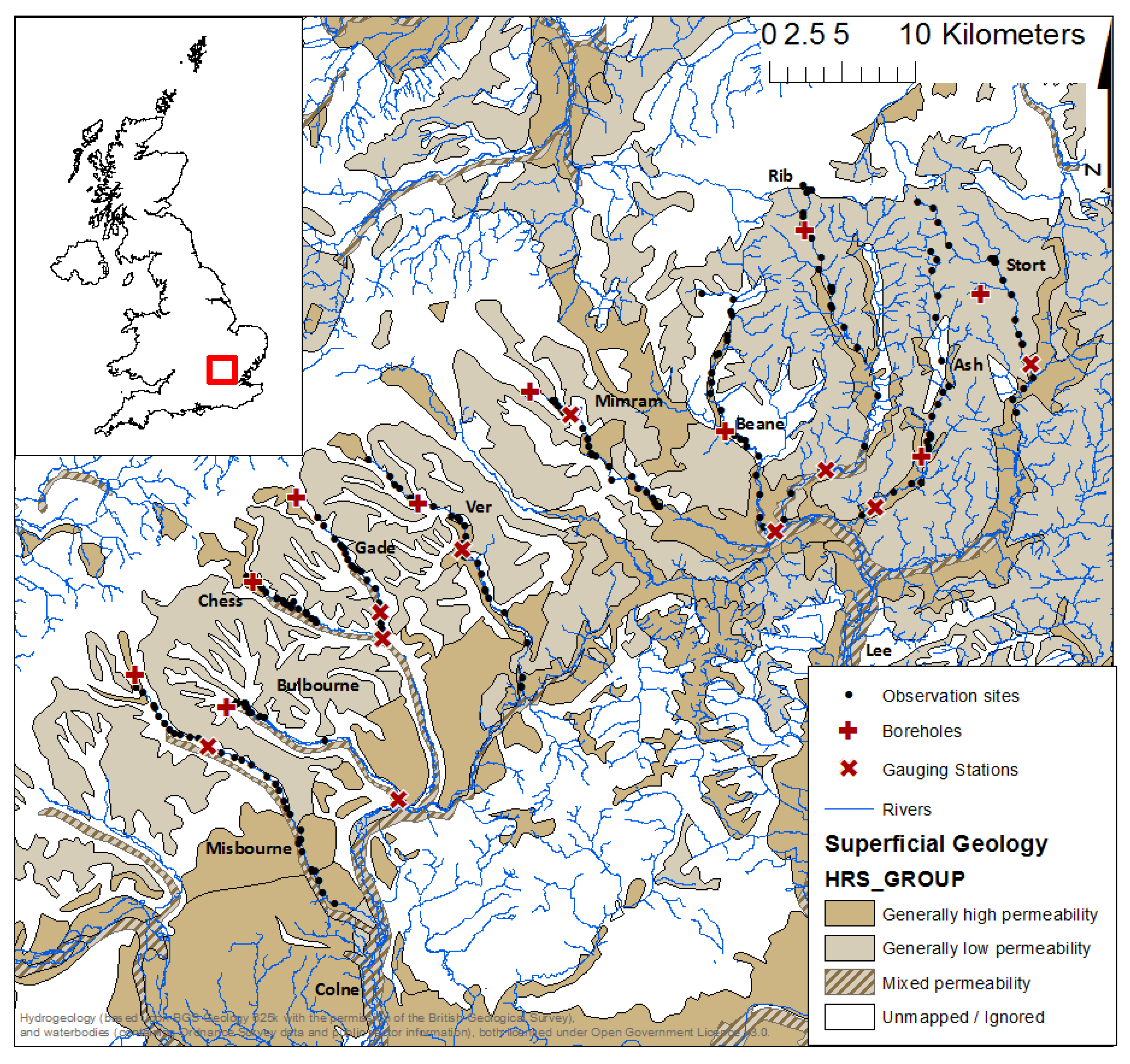
2.1. Study Area
2.2. Data
2.2.1. Hydrological State
2.2.2. Explanatory Data
2.3. Methods
2.3.1. Partial Proportional Odds
2.3.2. Parameter Estimation
2.3.3. Evaluation Metrics
2.3.4. Data Visualisation
3. Results
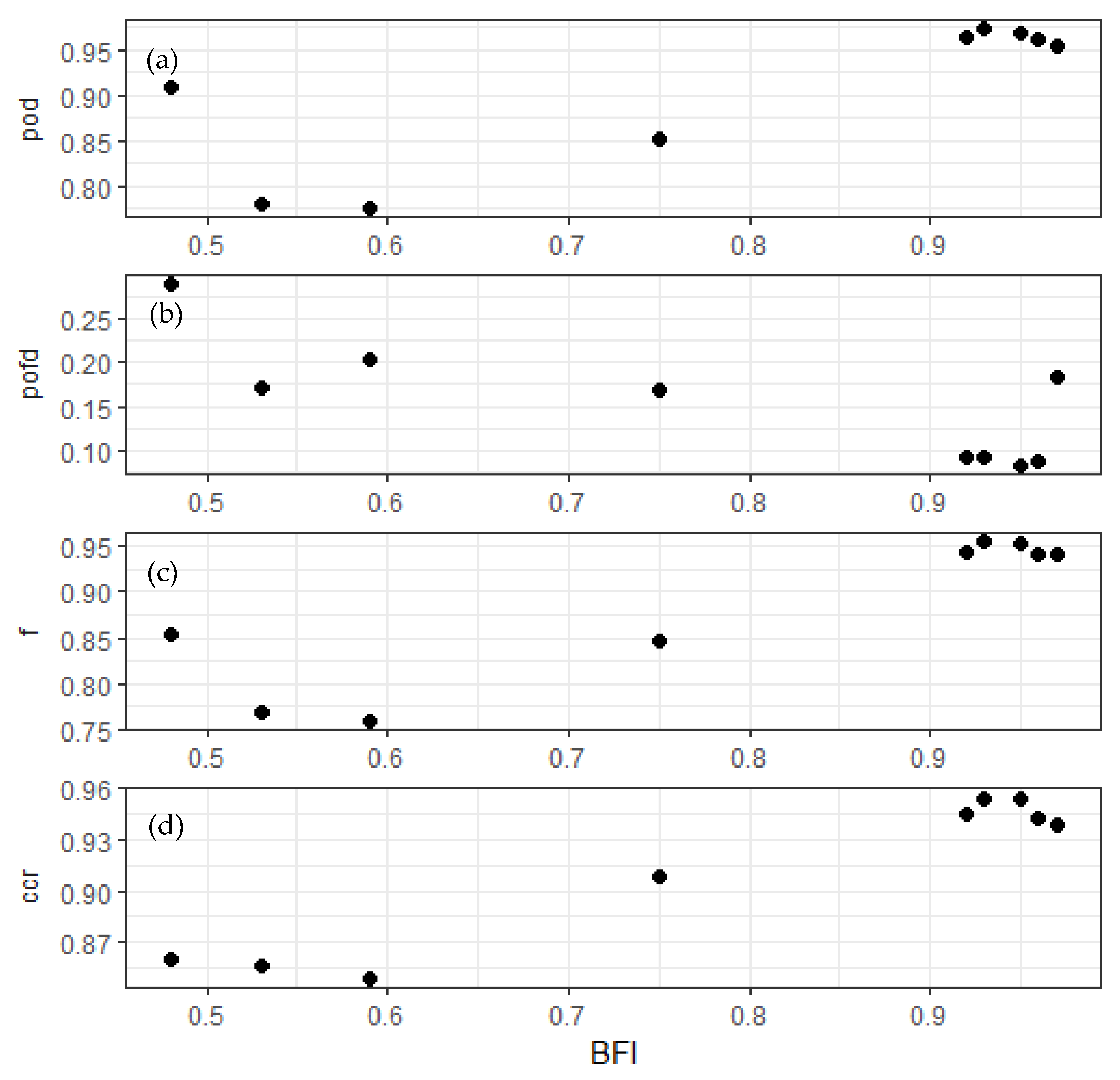
3.1. Overall Performance
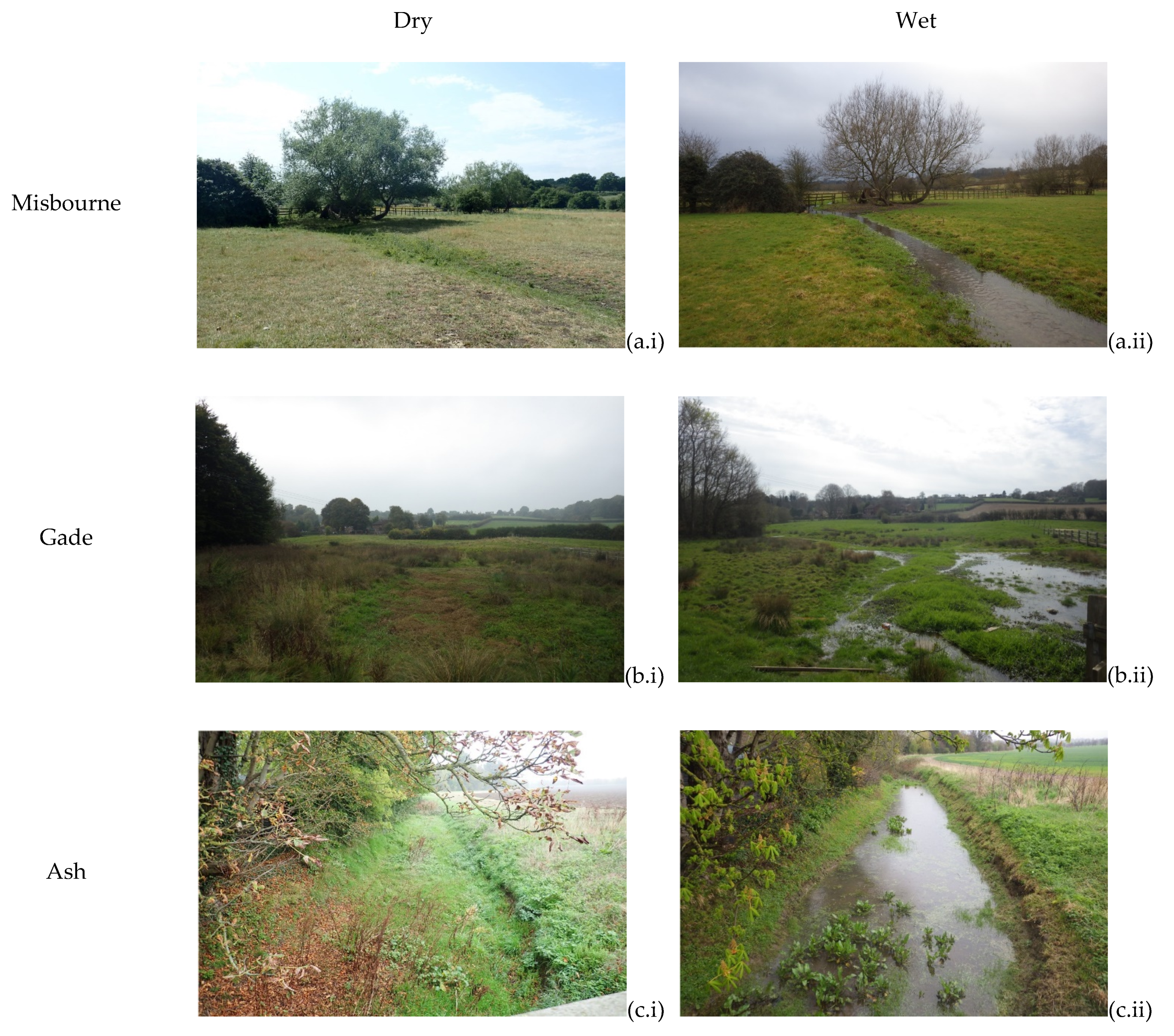
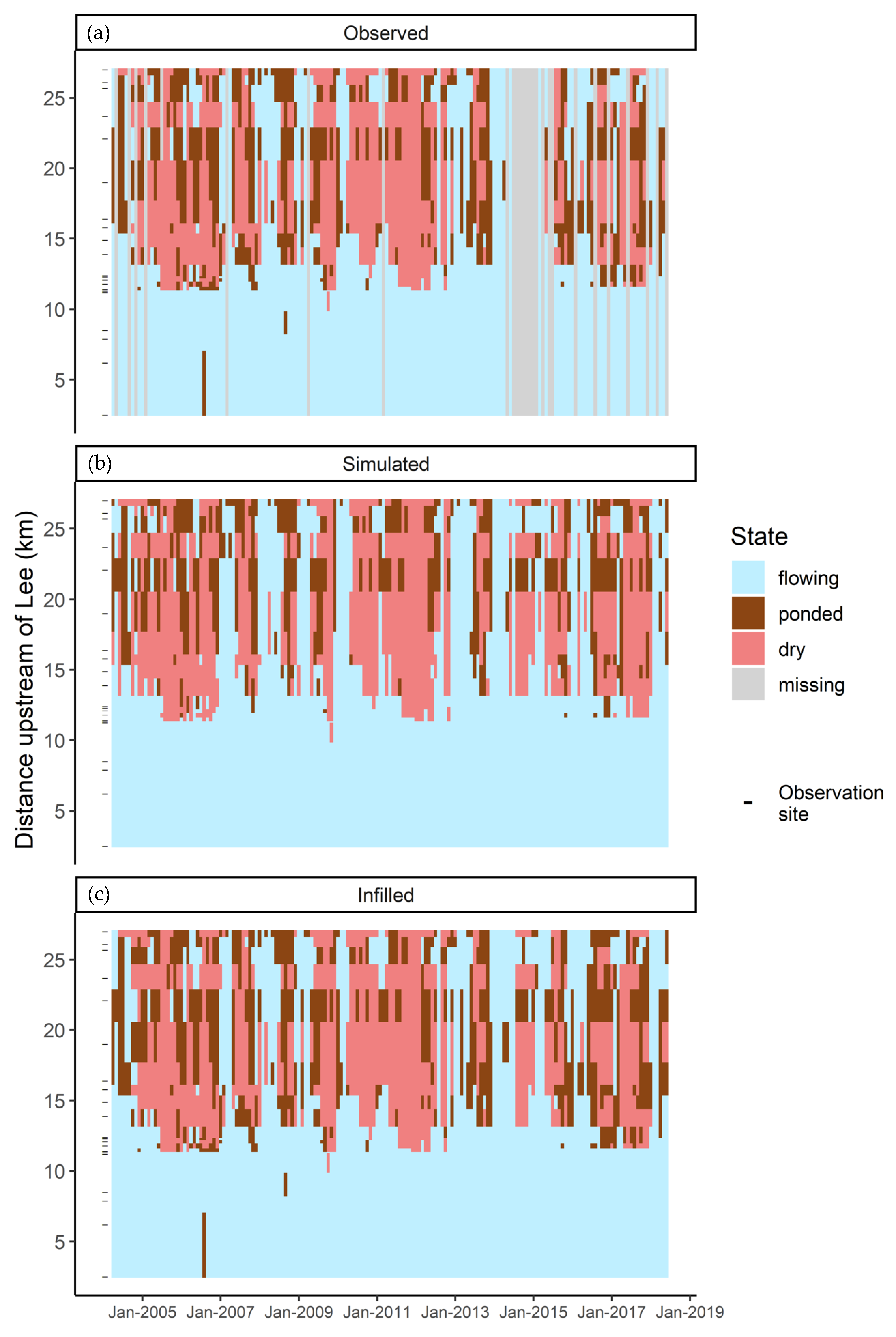
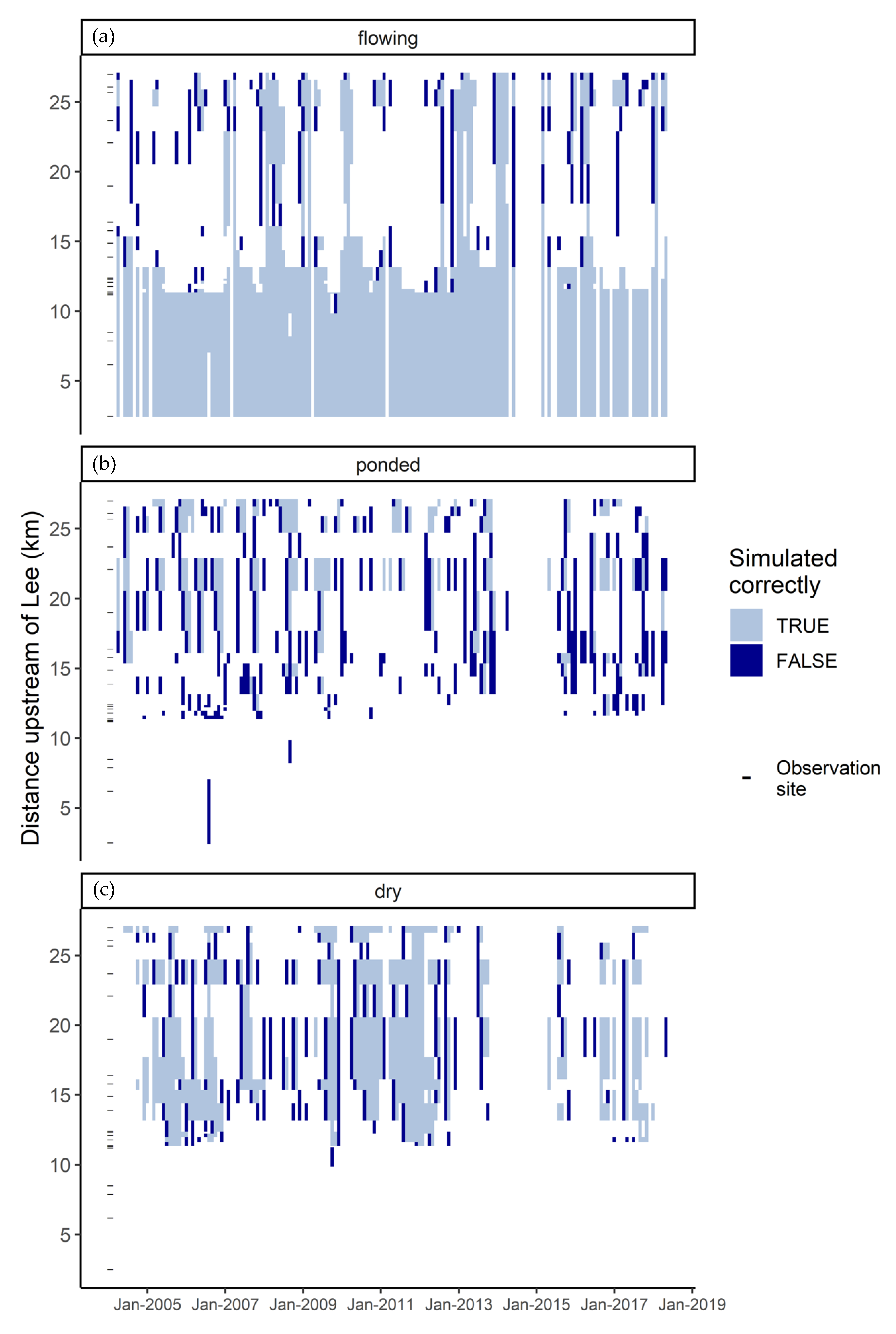
3.2. Gade
3.3. Misbourne
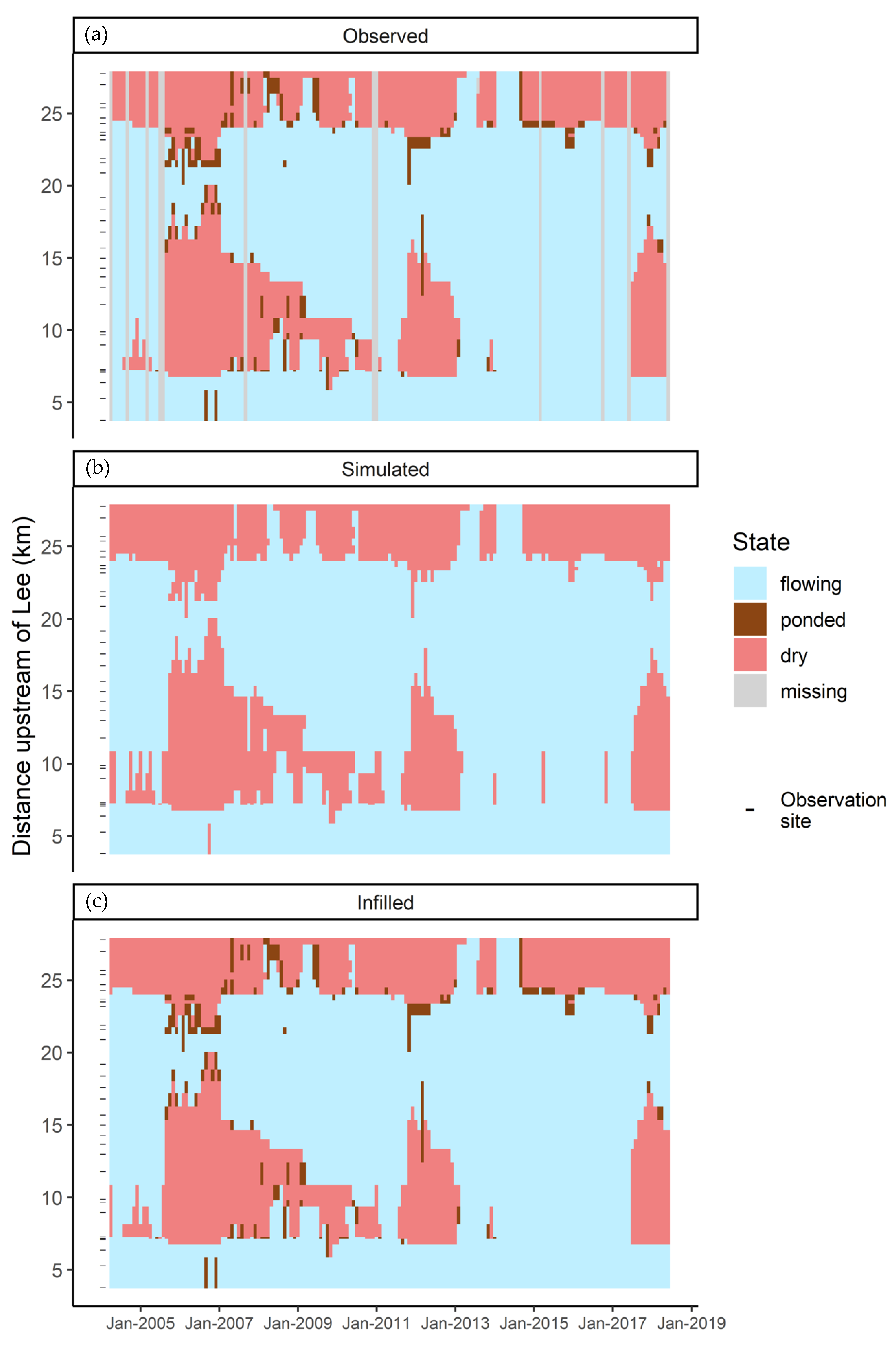
3.4. Ash
4. Discussion
4.1. Controls on Model Performance
4.2. Influence of Modelling Approach
4.3. Suitability for Infilling
4.4. Challenges and Limitations
4.5. Potential for Future Applications
5. Conclusions
Author Contributions
Funding
Institutional Review Board Statement
Informed Consent Statement
Data Availability Statement
Acknowledgments
Conflicts of Interest
Abbreviations
| AIC | Akaike’s Information Criterion |
| BFI | Base Flow Index |
| CCR | Correct Classification Rate |
| CLM | Cumulative Logit Model |
| IRES | Intermittent Rivers and Ephemeral Streams |
| m AOD | meters Above Ordnance Datum |
| POD | Probability of Detection |
| POFD | Probability of False Detection |
References
- Datry, T.; Larned, S.T.; Tockner, K. Intermittent Rivers: A Challenge for Freshwater Ecology. Bioscience 2014, 64, 229–235. [Google Scholar] [CrossRef] [Green Version]
- Smith, H.; Wood, P.J.; Gunn, J. The influence of habitat structure and flow permanence on invertebrate communities in karst spring systems. Hydrobiologia 2003, 510, 53–66. [Google Scholar] [CrossRef]
- Stubbington, R. The hyporheic zone as an invertebrate refuge: A review of variability in space, time, taxa and behaviour. Mar. Freshw. Res. 2012, 63, 293. [Google Scholar] [CrossRef] [Green Version]
- Datry, T.; Larned, S.T.; Fritz, K.M.; Bogan, M.T.; Wood, P.J.; Meyer, E.I.; Santos, A.N. Broad-scale patterns of invertebrate richness and community composition in temporary rivers: Effects of flow intermittence. Ecography 2014, 37, 94–104. [Google Scholar] [CrossRef] [Green Version]
- Leigh, C.; Datry, T. Drying as a primary hydrological determinant of biodiversity in river systems: A broad-scale analysis. Ecography 2017, 40, 487–499. [Google Scholar] [CrossRef] [Green Version]
- Stubbington, R.; England, J.; Wood, P.J.; Sefton, C.E.M. Temporary streams in temperate zones: Recognizing, monitoring and restoring transitional aquatic-terrestrial ecosystems. WIREs Water 2017, 4, e1223. [Google Scholar] [CrossRef] [Green Version]
- Hill, M.J.; Milner, V.S. Ponding in intermittent streams: A refuge for lotic taxa and a habitat for newly colonising taxa? Sci. Total Environ. 2018, 628–629, 1308–1316. [Google Scholar] [CrossRef] [PubMed]
- Datry, T.; Pella, H.; Leigh, C.; Bonada, N.; Hugueny, B. A landscape approach to advance intermittent river ecology. Freshw. Biol. 2016, 61, 1200–1213. [Google Scholar] [CrossRef] [Green Version]
- Leibowitz, S.G.; Wigington, P.J.; Rains, M.C.; Downing, D.M. Non-navigable streams and adjacent wetlands: Addressing science needs following the Supreme Court’s Rapanos decision. Front. Ecol. Environ. 2008, 6, 364–371. [Google Scholar] [CrossRef] [Green Version]
- Fritz, K.; Cid, N.; Autrey, B. Governance, legislation, and protection of intermittent rivers and ephemeral streams. In Intermittent Rivers and Ephemeral Streams; Elsevier: Amsterdam, The Netherlands, 2017; pp. 477–507. ISBN 9780128038352. [Google Scholar]
- Skoulikidis, N.T.; Sabater, S.; Datry, T.; Morais, M.M.; Buffagni, A.; Dörflinger, G.; Zogaris, S.; Del Mar Sánchez-Montoya, M.; Bonada, N.; Kalogianni, E.; et al. Non-perennial Mediterranean rivers in Europe: Status, pressures, and challenges for research and management. Sci. Total Environ. 2017, 577, 1–18. [Google Scholar] [CrossRef]
- Costigan, K.H.; Jaeger, K.L.; Goss, C.W.; Fritz, K.M.; Goebel, P.C. Understanding controls on flow permanence in intermittent rivers to aid ecological research: Integrating meteorology, geology and land cover. Ecohydrology 2016, 9, 1141–1153. [Google Scholar] [CrossRef]
- Larned, S.T.; Datry, T.; Arscott, D.B.; Tockner, K. Emerging concepts in temporary-river ecology. Freshw. Biol. 2010, 55, 717–738. [Google Scholar] [CrossRef]
- Van Meerveld, H.J.I.; Sauquet, E.; Gallart, F.; Sefton, C.; Seibert, J.; Bishop, K. Aqua temporaria incognita. Hydrol. Process. 2020. [Google Scholar] [CrossRef]
- Jensen, C.K.; McGuire, K.J.; Shao, Y.; Andrew Dolloff, C. Modeling wet headwater stream networks across multiple flow conditions in the Appalachian Highlands. Earth Surf. Process. Landf. 2018, 43, 2762–2778. [Google Scholar] [CrossRef] [Green Version]
- Yu, S.; Bond, N.R.; Bunn, S.E.; Xu, Z.; Kennard, M.J. Quantifying spatial and temporal patterns of flow intermittency using spatially contiguous runoff data. J. Hydrol. 2018, 559, 861–872. [Google Scholar] [CrossRef] [Green Version]
- Kaplan, N.H.; Blume, T.; Weiler, M. Predicting probabilities of streamflow intermittency across a temperate mesoscale catchment. Hydrol. Earth Syst. Sci. 2020, 24, 5453–5472. [Google Scholar] [CrossRef]
- Beaufort, A.; Carreau, J.; Sauquet, E. A classification approach to reconstruct local daily drying dynamics at headwater streams. Hydrol. Process. 2019. [Google Scholar] [CrossRef]
- González-Ferreras, A.M.; Barquín, J. Mapping the temporary and perennial character of whole river networks. Water Resour. Res. 2017, 53, 6709–6724. [Google Scholar] [CrossRef] [Green Version]
- Jaeger, K.L.; Sando, R.; McShane, R.R.; Dunham, J.B.; Hockman-Wert, D.P.; Kaiser, K.E.; Hafen, K.; Risley, J.C.; Blasch, K.W. Probability of Streamflow Permanence Model (PROSPER): A spatially continuous model of annual streamflow permanence throughout the Pacific Northwest. J. Hydrol. X 2019, 2, 100005. [Google Scholar] [CrossRef]
- Yu, S.; Bond, N.R.; Bunn, S.E.; Kennard, M.J. Development and application of predictive models of surface water extent to identify aquatic refuges in Eastern Australian temporary stream networks. Water Resour. Res. 2019, 55, 9639–9655. [Google Scholar] [CrossRef] [Green Version]
- Bond, N.R.; Kennard, M.J. Prediction of hydrologic characteristics for ungauged catchments to support hydroecological modeling. Water Resour. Res. 2017. [Google Scholar] [CrossRef]
- Bonada, N.; Cañedo-Argüelles, M.; Gallart, F.; von Schiller, D.; Fortuño, P.; Latron, J.; Llorens, P.; Múrria, C.; Soria, M.; Vinyoles, D.; et al. Conservation and management of isolated pools in temporary rivers. Water 2020, 12, 2870. [Google Scholar] [CrossRef]
- Drummond, L.R.; McIntosh, A.R.; Larned, S.T. Invertebrate community dynamics and insect emergence in response to pool drying in a temporary river. Freshw. Biol. 2015, 60, 1596–1612. [Google Scholar] [CrossRef]
- Kerezsy, A.; Gido, K.; Magalhaes, M.F.; Skelton, P.H. The biota of intermittent rivers and ephemeral streams: Fishes. In Intermittent Rivers and Ephemeral Streams: Ecology and Management; Datry, T., Bonada, N., Boulton, A.J., Eds.; Elsevier, Inc.: Cambridge, MA, USA, 2017; pp. 273–298. [Google Scholar]
- Arthington, A.H.; Balcombe, S.R. Extreme flow variability and the ‘boom and bust’ ecology of fish in arid-zone floodplain rivers: A case history with implications for environmental flows, conservation and management. Ecohydrology 2011, 4, 708–720. [Google Scholar] [CrossRef] [Green Version]
- Stubbington, R.; England, J.; Acreman, M.; Wood, P.J.; Westwood, C.; Boon, P.; Mainstone, C.; Macadam, C.; Bates, A.; House, A.; et al. The Natural Capital of Temporary Rivers: Characterising the Value of Dynamic Aquatic-Terrestrial Habitats; Valuing Nature Natural Capital Synthesis Report VNP12; 2018; Available online: https://valuing-nature.net/TemporaryRiverNC (accessed on 11 February 2021).
- Querner, E.P.; Froebrich, J.; Gallart, F.; Cazemier, M.M.; Tzoraki, O. Simulating streamflow variability and aquatic states in temporary streams using a coupled groundwater-surface water model. Hydrol. Sci. J. 2016, 61, 146–161. [Google Scholar] [CrossRef]
- Sefton, C.E.M.; Parry, S.; England, J.; Angell, G. Visualising and quantifying the variability of hydrological state in intermittent rivers. Fundam. Appl. Limnol. 2019. [Google Scholar] [CrossRef]
- Gustard, A.; Bullock, A.; Dixon, J.M. Low Flow Estimation in the United Kingdom (IH Report); Centre for Ecology & Hydrology: Wallingford, UK, 1992; p. 292. ISBN 0948540451. [Google Scholar]
- National River Flow Archive. Available online: https://nrfa.ceh.ac.uk/ (accessed on 18 September 2020).
- Gallart, F.; Prat, N.; García-Roger, E.M.; Latron, J.; Rieradevall, M.; Llorens, P.; Barberá, G.G.; Brito, D.; De Girolamo, A.M.; Lo Porto, A.; et al. A novel approach to analysing the regimes of temporary streams in relation to their controls on the composition and structure of aquatic biota. Hydrol. Earth Syst. Sci. 2012, 16, 3165–3182. [Google Scholar] [CrossRef] [Green Version]
- Environment Agency: Groundwater and Hydrology. Monthly Water Situation Report: Hertfordshire and North London. 2021. Available online: https://assets.publishing.service.gov.uk/government/uploads/system/uploads/attachment_data/file/951151/Hertfordshire_and_North_London_Water_Situation_Report_December_2020.pdf (accessed on 21 January 2021).
- Hyoms, C.M. Development of a Soil Moisture Model for the Estimation of Percolation. Ph.D. Thesis, The City University, London, UK, 1980. [Google Scholar]
- Agresti, A. Categorical Data Analysis; John Wiley & Sons, Inc.: Hoboken, NJ, USA, 2002; pp. 274–282. ISBN 0471249688. [Google Scholar]
- Christensen, R.H.B. Regression Models for Ordinal Data. R Package Version 2019.12-10. Available online: https://CRAN.R-project.org/package=ordinal (accessed on 18 September 2020).
- Hargis, C.D.; Bissonette, J.A.; David, J.L. The Behavior of Landscape Metrics Commonly Used in the Study of Habitat Fragmentation; Springer Science and Business Media LLC: Berlin/Heidelberg, Germany, 1998. [Google Scholar] [CrossRef]
- Snelder, T.H.; Datry, T.; Lamouroux, N.; Larned, S.T.; Sauquet, E.; Pella, H.; Catalogne, C. Regionalization of patterns of flow intermittence from gauging station records. Hydrol. Earth Syst. Sci. 2013, 17, 2685–2699. [Google Scholar] [CrossRef] [Green Version]
- D’Ambrosio, E.; De Girolamo, A.M.; Barca, E.; Ielpo, P.; Rulli, M.C. Characterising the hydrological regime of an ungauged temporary river system: A case study. Environ. Sci. Pollut. Res. Int. 2017, 24, 13950–13966. [Google Scholar] [CrossRef]
- Steward, A.L.; von Schiller, D.; Tockner, K.; Marshall, J.C.; Bunn, S.E. When the river runs dry: Human and ecological values of dry riverbeds. Front. Ecol. Environ. 2012, 10, 202–209. [Google Scholar] [CrossRef] [Green Version]
- Leigh, C.; Boulton, A.J.; Courtwright, J.L.; Fritz, K.; May, C.L.; Walker, R.H.; Datry, T. Ecological research and management of intermittent rivers: An historical review and future directions. Freshw. Biol. 2016, 61, 1181–1199. [Google Scholar] [CrossRef]
- Sarremejane, R.; England, J.; Sefton, C.E.M.; Parry, S.; Eastman, M.; Stubbington, R. Local and regional drivers influence how aquatic community diversity, resistance and resilience vary in response to drying. Oikos 2020. [Google Scholar] [CrossRef]
- CrowdWater. Available online: https://crowdwater.ch/ (accessed on 12 November 2020).
- Tramblay, Y.; Rutkowska, A.; Sauquet, E.; Sefton, C.; Laaha, G.; Osuch, M.; Albuquerque, T.; Alves, M.H.; Banasik, K.; Beaufort, A.; et al. Trends in flow intermittence for European rivers. Hydrol. Sci. J. 2021, 66, 37–49. [Google Scholar] [CrossRef]
- De Girolamo, A.M.; Bouraoui, F.; Baffagni, A.; Pappagallo, G.; Lo Porto, A. Hydrology under climate change in a temporary river system: Potential impact on water balance and flow regime. River Res. Appl. 2017, 33, 1219–1232. [Google Scholar] [CrossRef]
- Pumo, D.; Caracciolo, D.; Viola, F.; Noto, L.V. Climate change effects on the hydrological regime of small non-perennial river basins. Sci. Total Environ. 2016, 542, 76–92. [Google Scholar] [CrossRef] [PubMed]


| Factor | Description |
|---|---|
| Flow | Mean flow in the month of the hydrological state being simulated (m3s−1) |
| Groundwater | Mean level of water table in the month of the hydrological state being simulated (m AOD) |
| Precipitation | Mean precipitation in the month of the hydrological state being simulated (mm) |
| Proportion of days with >0 mm precipitation in the month of the hydrological state being simulated | |
| Mean percolation in the month of the hydrological state being simulated (mm) | |
| Proportion of days with >0 mm percolation in the month of the hydrological state being simulated | |
| Seasonality | Categorical month of hydrological state being simulated |
| Site | Distance downstream to the confluence (km) |
| State | Hydrological state (flowing, ponded, dry) in the previous and following months |
| River | Flow Gauging Station | Borehole | ||
|---|---|---|---|---|
| Name | National Grid Reference | Name | National Grid Reference | |
| Misbourne | Little Missenden | SU9342198458 | Woodlands Park | SP8846703308 |
| Chess | Rickmansworth | TQ0657394809 | Wayside | SP9477001065 |
| Bulbourne | Two Waters | TL0550405809 | Dudswell | SP9659009682 |
| Gade | Bury Mill | TL0532607648 | Dagnall OBH | SP9960015540 |
| Ver | Redbourn | TL1091611904 | River Hill Dip | TL0798015060 |
| Mimram | Whitwell | TL1841021210 | Lilley Bottom Dip | TL1569022760 |
| Beane | Hartham Park | TL3250313143 | Watton at Stone | TL2910220042 |
| Rib | Wadesmill | TL3599017444 | Lower Farm Buckland | TL3457033890 |
| Ash | Wareside Mardock | TL3936014840 | Much Hadham | TL4261218286 |
| Stort | Stansted Springs | TL5003924731 | Berden Hall | TL4669429548 |
| POD | POFD | f-Score | CCR | |
|---|---|---|---|---|
| Misbourne | 0.961 | 0.088 | 0.942 | 0.942 |
| Chess | 0.968 | 0.083 | 0.954 | 0.954 |
| Bulbourne | 0.958 | 0.116 | 0.935 | 0.935 |
| Gade | 0.973 | 0.093 | 0.955 | 0.955 |
| Ver | 0.964 | 0.093 | 0.944 | 0.949 |
| Mimram | 0.954 | 0.183 | 0.941 | 0.939 |
| Beane * | 0.852 | 0.168 | 0.848 | 0.909 |
| Rib * | 0.775 | 0.203 | 0.759 | 0.849 |
| Ash * | 0.780 | 0.170 | 0.768 | 0.857 |
| Stort * | 0.908 | 0.288 | 0.855 | 0.861 |
| River | Misbourne | Chess | Bulbourne | Gade | Ver | Mimram | Beane | Rib | Ash | Stort |
|---|---|---|---|---|---|---|---|---|---|---|
| Flow average | X | X | X | X | X | X * | X * | X * | X * | |
| Average water table height | X | X | X | X | X | X | X * | X | X | X |
| Average precipitation | X | X * | X | X | ||||||
| Precipitation frequency | X | X | X | X | X | |||||
| Average percolation | X | X | X | X | X* | |||||
| Percolation frequency | X | X | X | X * | X | X | X | |||
| Distance upstream of confluence | X | X | X | X | X | X | X * | X | X * | X * |
| Month | X | X | X | X | X * | X | ||||
| Previous month state | X | X | X | X | X | X | X * | X * | X * | X * |
| Following month state | X | X | X | X | X | X | X * | X * | X * | X * |
Publisher’s Note: MDPI stays neutral with regard to jurisdictional claims in published maps and institutional affiliations. |
© 2021 by the authors. Licensee MDPI, Basel, Switzerland. This article is an open access article distributed under the terms and conditions of the Creative Commons Attribution (CC BY) license (http://creativecommons.org/licenses/by/4.0/).
Share and Cite
Eastman, M.; Parry, S.; Sefton, C.; Park, J.; England, J. Reconstructing Spatiotemporal Dynamics in Hydrological State Along Intermittent Rivers. Water 2021, 13, 493. https://doi.org/10.3390/w13040493
Eastman M, Parry S, Sefton C, Park J, England J. Reconstructing Spatiotemporal Dynamics in Hydrological State Along Intermittent Rivers. Water. 2021; 13(4):493. https://doi.org/10.3390/w13040493
Chicago/Turabian StyleEastman, Michael, Simon Parry, Catherine Sefton, Juhyun Park, and Judy England. 2021. "Reconstructing Spatiotemporal Dynamics in Hydrological State Along Intermittent Rivers" Water 13, no. 4: 493. https://doi.org/10.3390/w13040493
APA StyleEastman, M., Parry, S., Sefton, C., Park, J., & England, J. (2021). Reconstructing Spatiotemporal Dynamics in Hydrological State Along Intermittent Rivers. Water, 13(4), 493. https://doi.org/10.3390/w13040493