
Numerical Simulation of Local Scour around Three Cylindrical Piles in a Tandem Arrangement


Abstract
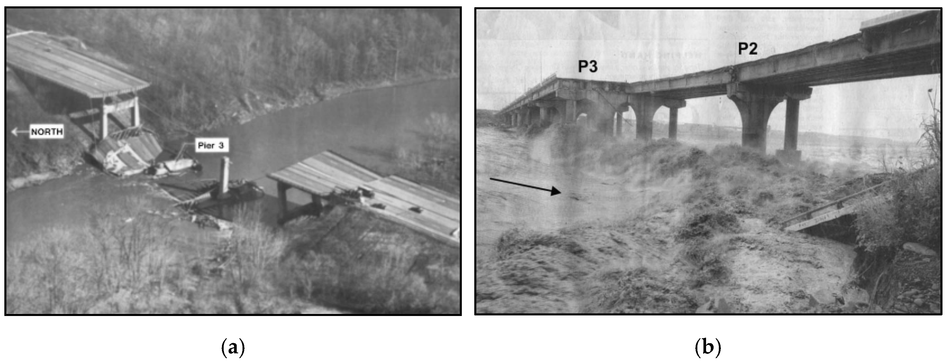
:1. Introduction
2. Numerical Method
2.1. Governing Equations
2.2. Turbulence Model
2.3. Sediment Transport Model
2.3.1. Critical Shields Number
2.3.2. Bed-Load Transport
2.3.3. Maximum Packing Fraction
2.3.4. Bed Shear Stress
2.3.5. Sediment Characteristics
2.4. Meshing
2.5. Boundary Conditions
3. Verification of the Present Model
3.1. Experimental Setup
3.2. Numerical Setup
3.2.1. Sediment Scour and Turbulence
3.2.2. Geometry and Meshing
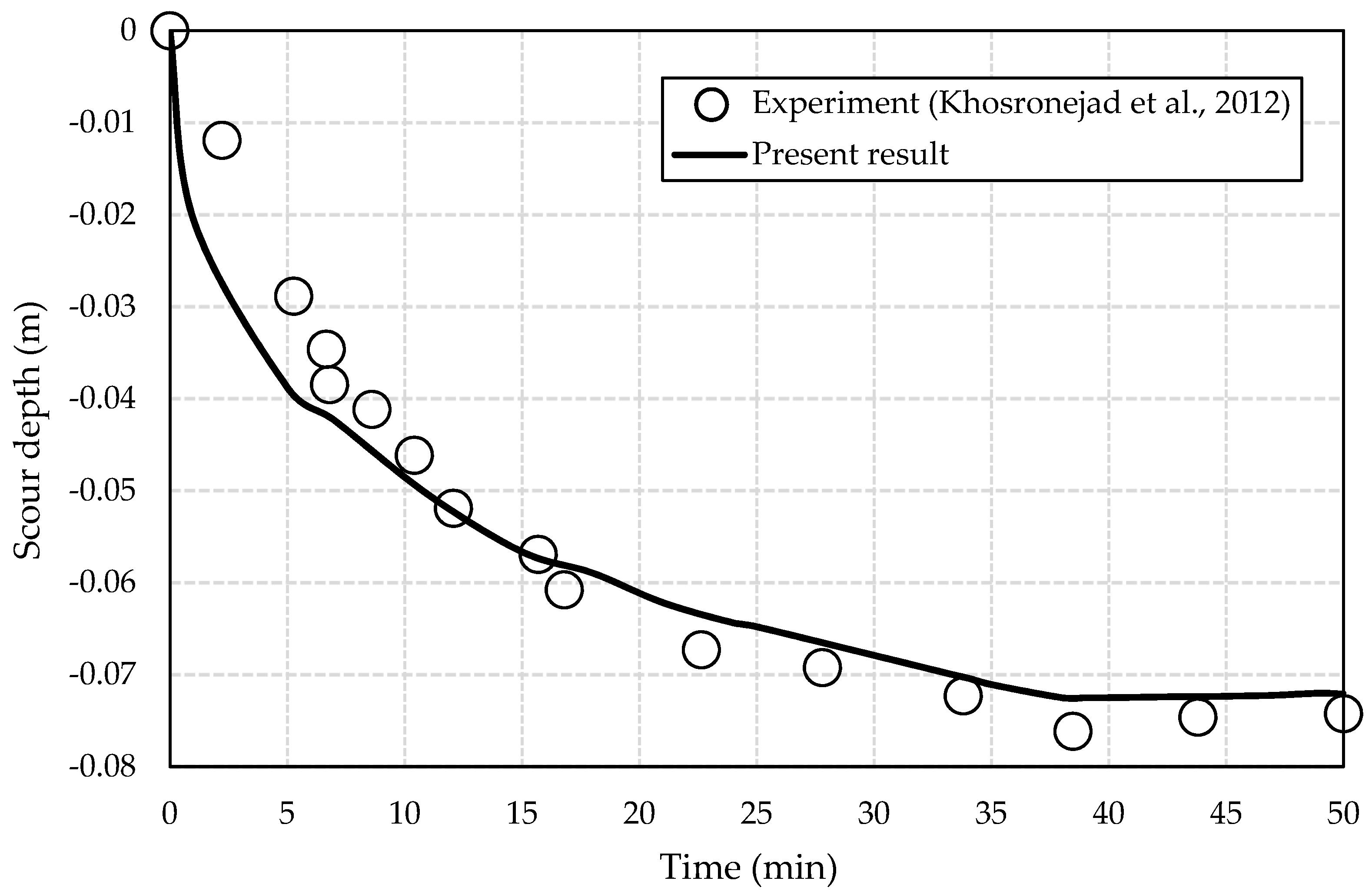
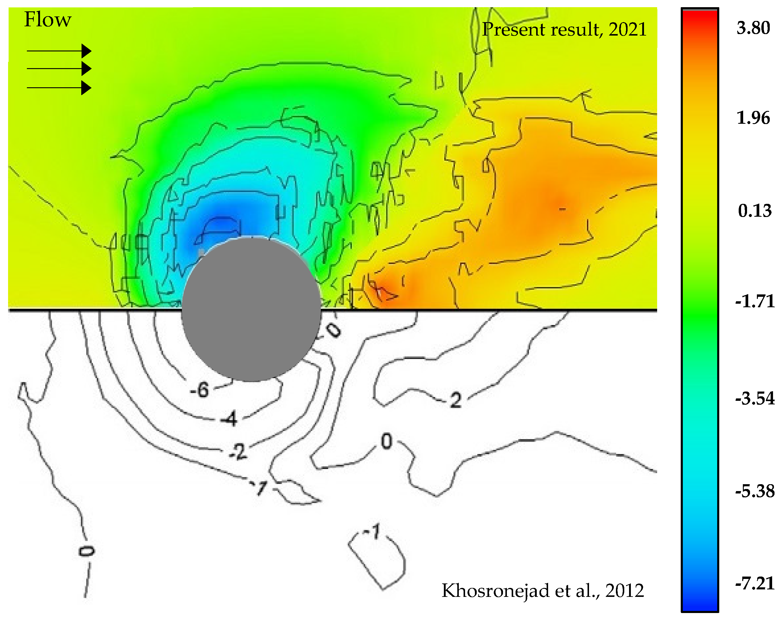
3.3. Validation Result
4. Numerical Simulation of Three Cylinders
4.1. Sediment Scour and Turbulence
4.2. Geometry and Meshing
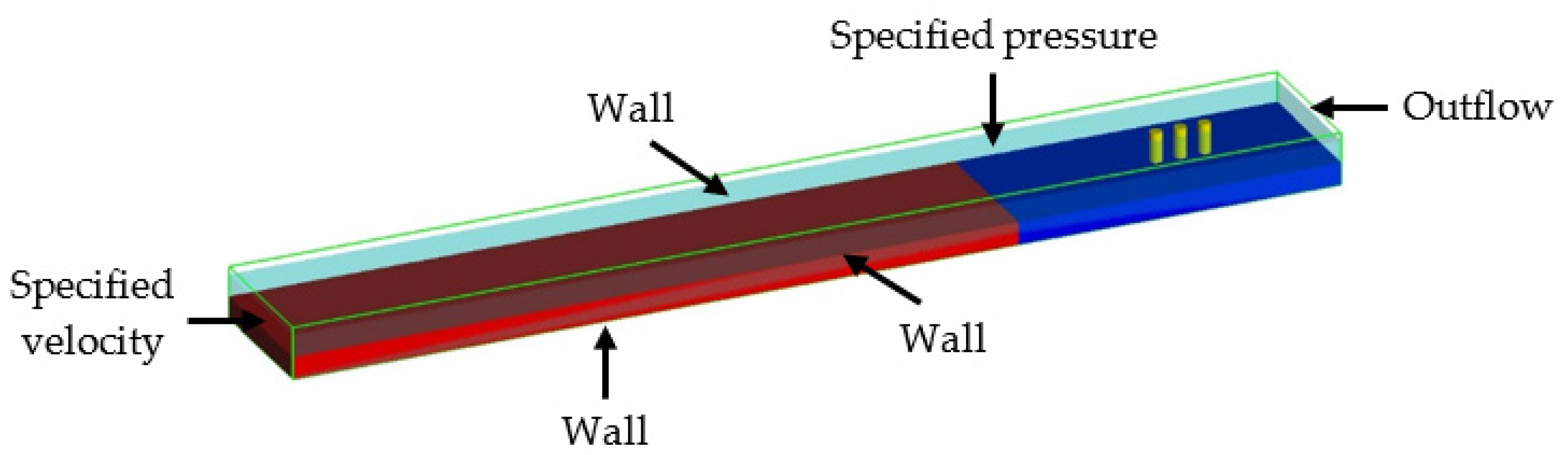
4.3. Boundary Conditions
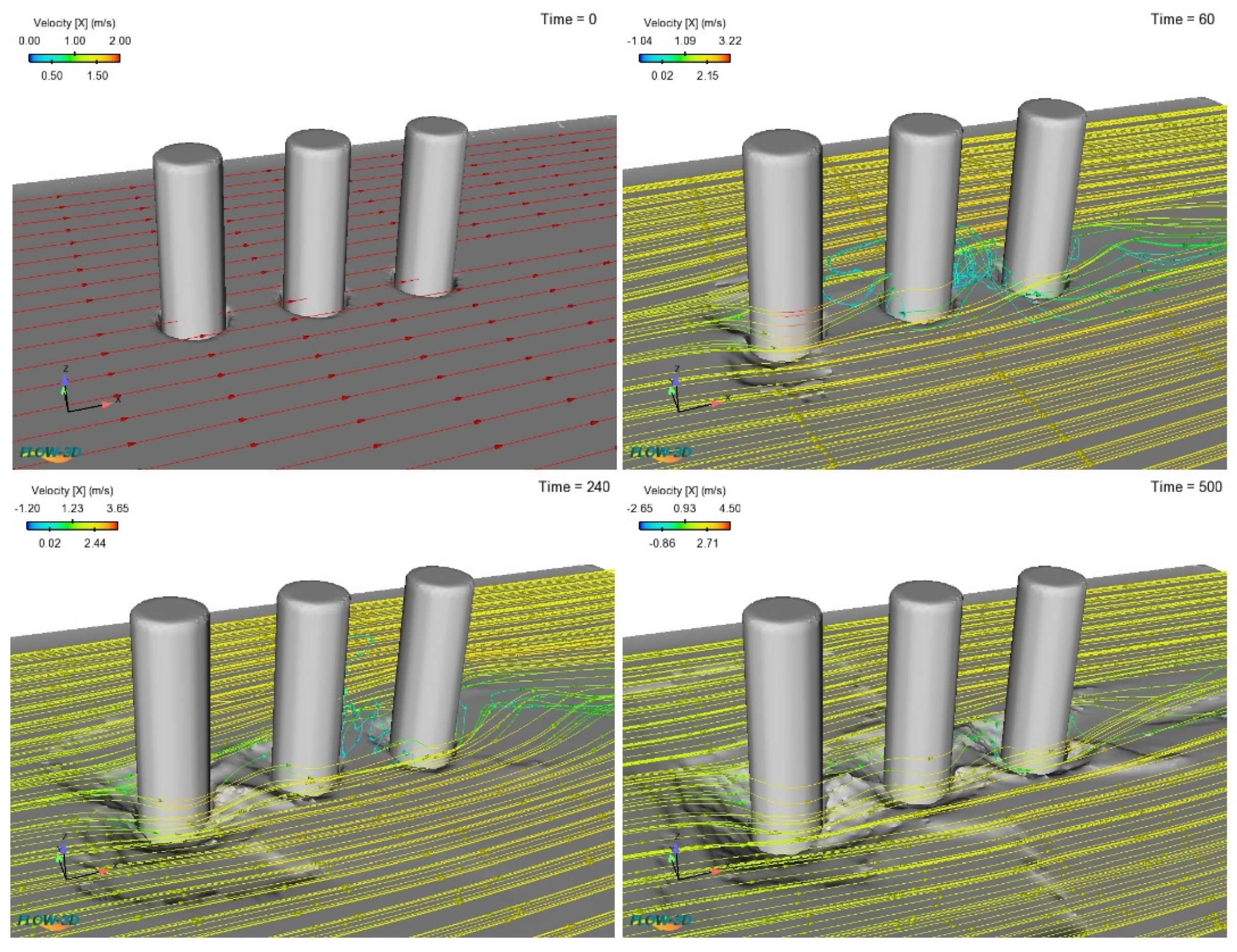
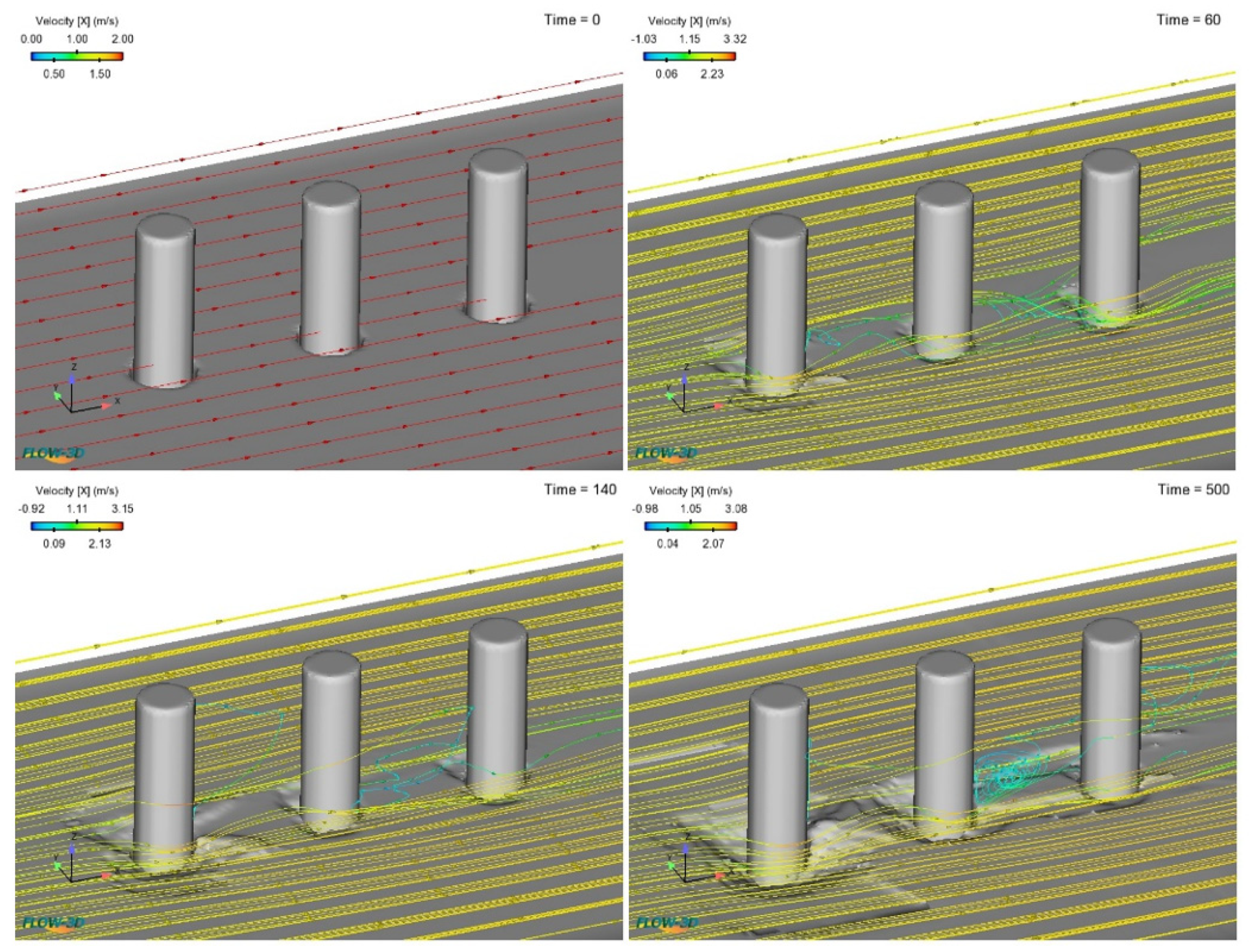
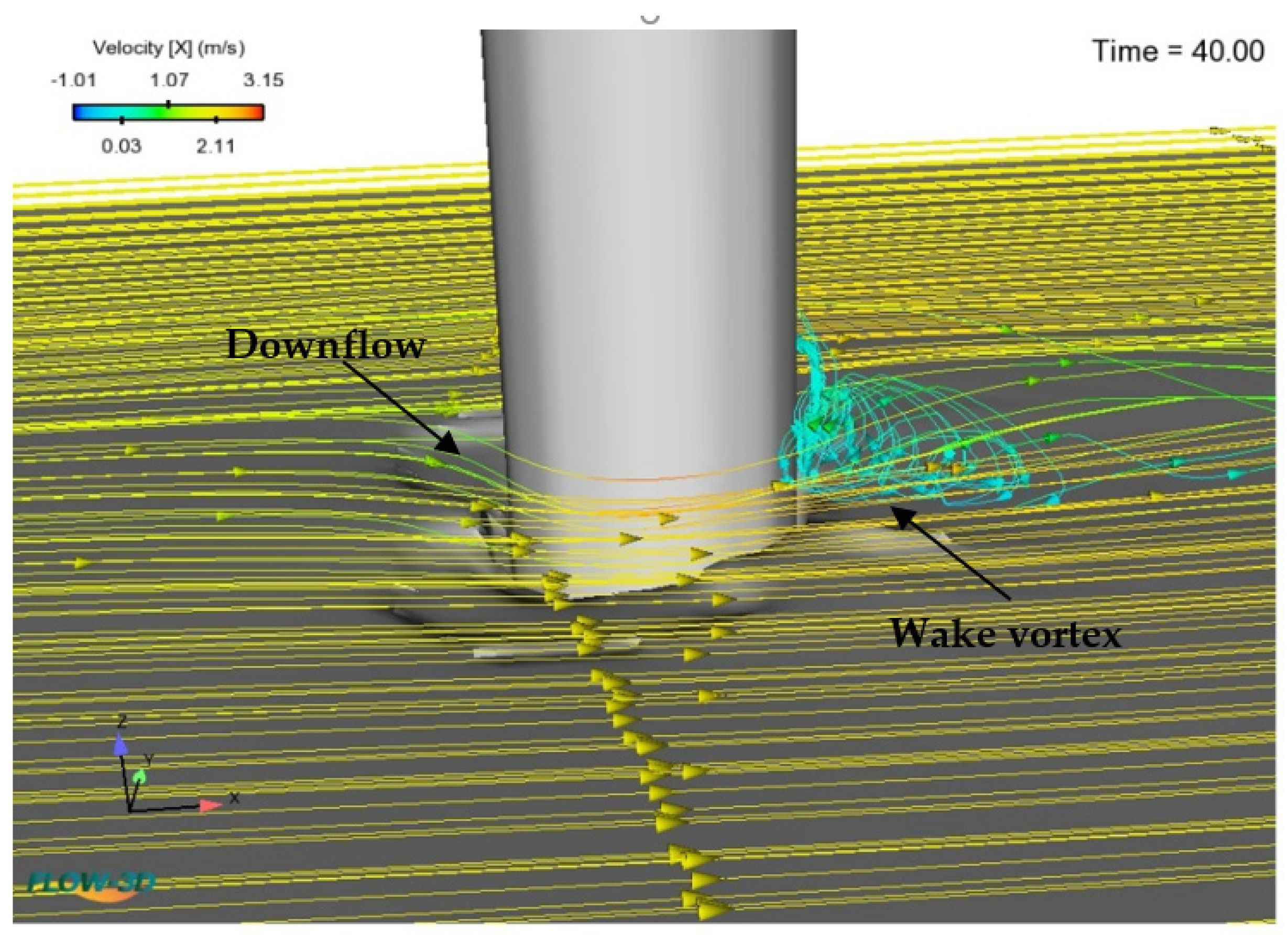
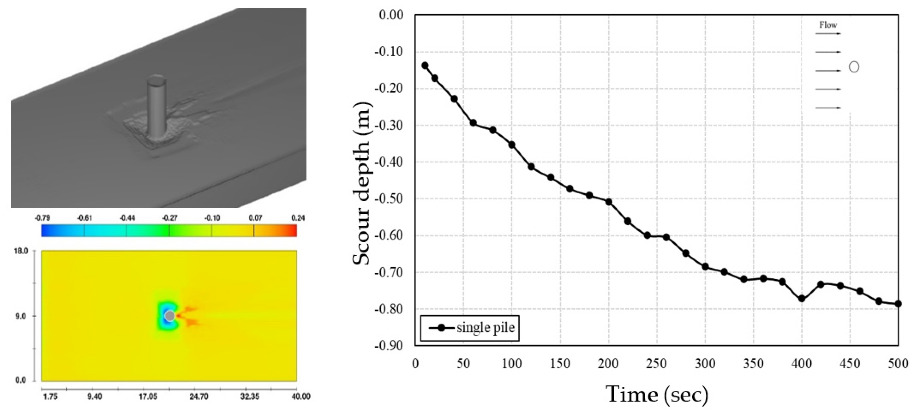
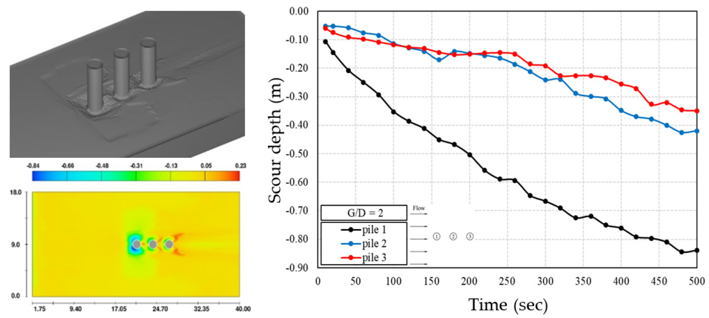
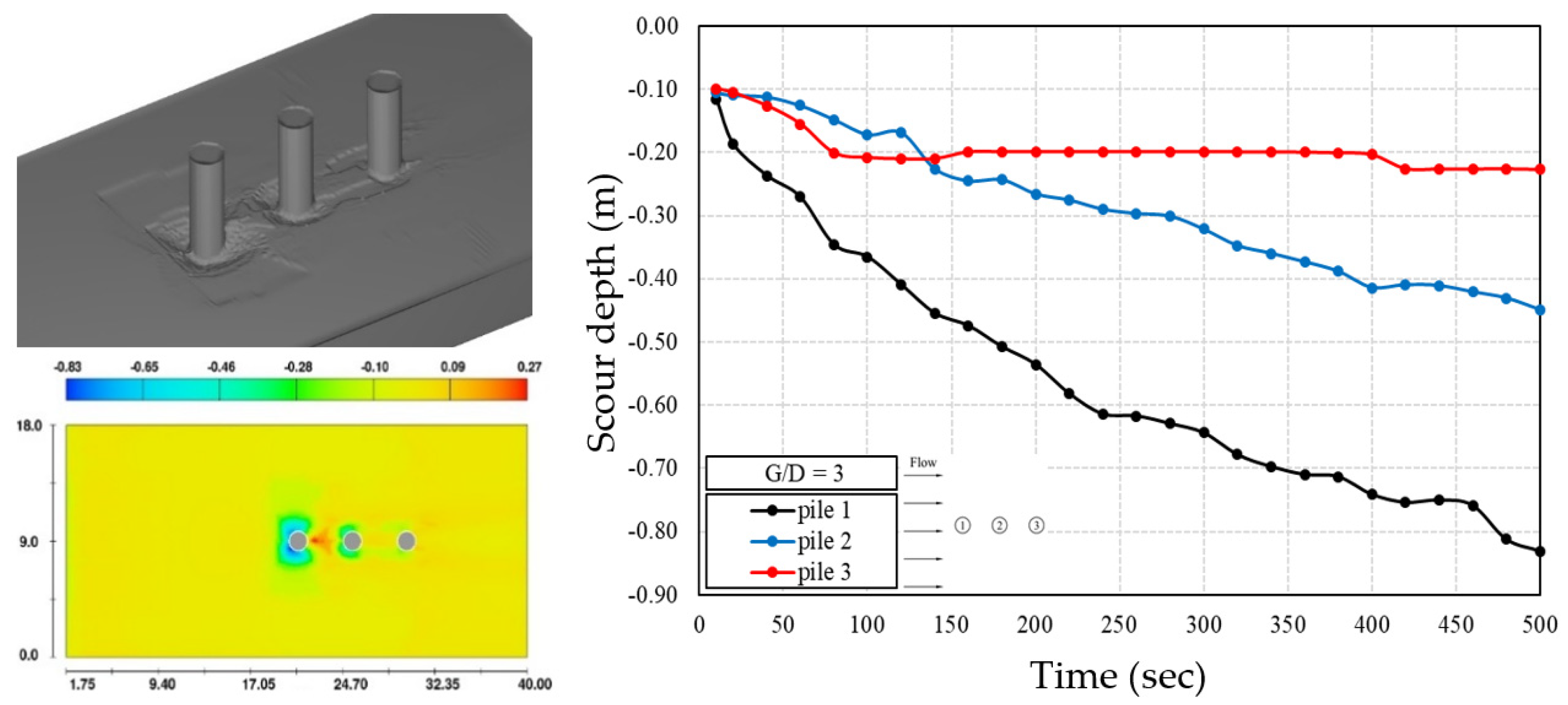
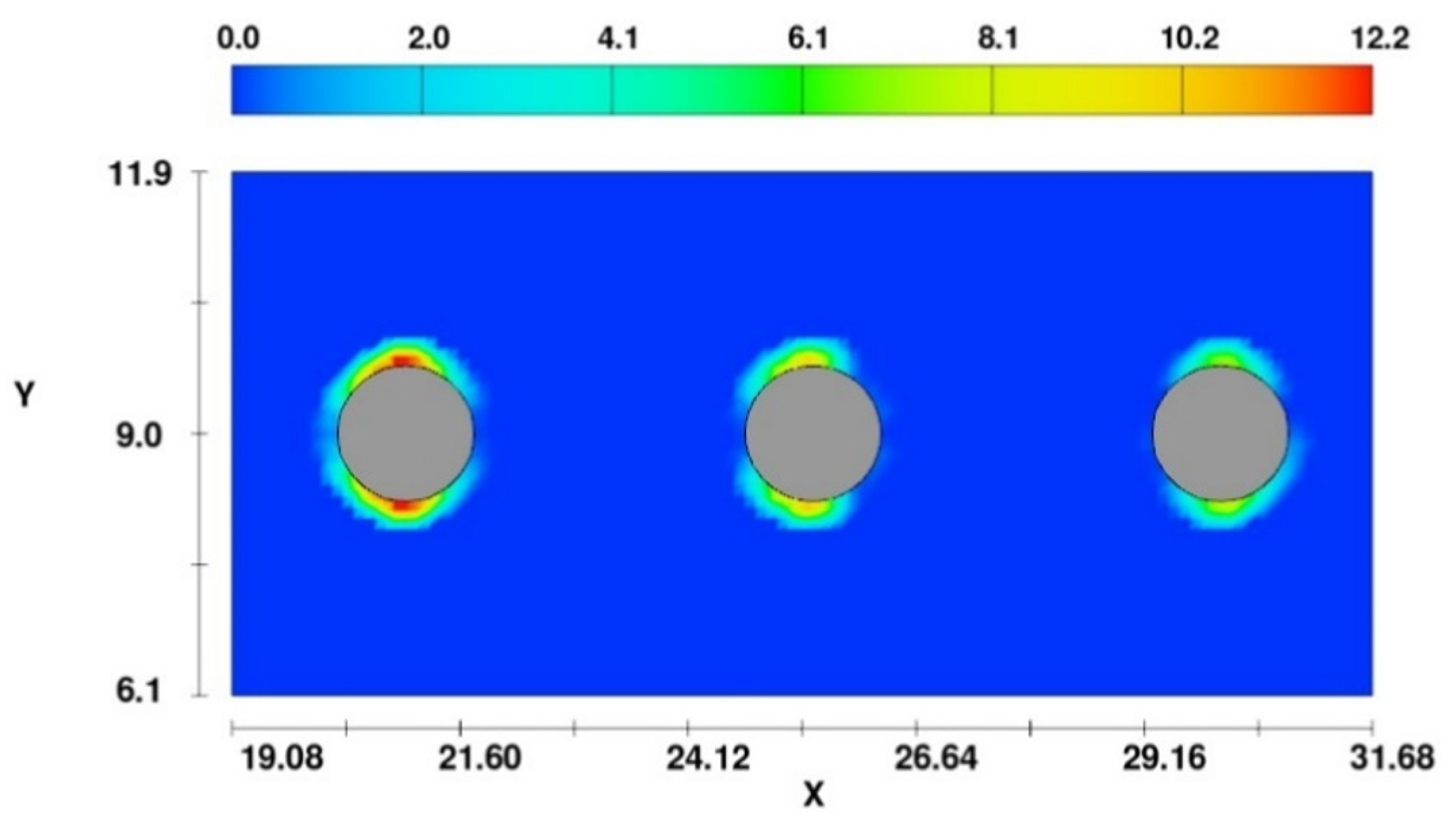
4.4. Numerical Results and Discussion
5. Conclusions
Author Contributions
Funding
Institutional Review Board Statement
Informed Consent Statement
Data Availability Statement
Conflicts of Interest
References
- Basack, S. Analysis and design of offshore pile foundation. In Advanced Materials Research; Trans Tech Publications, Ltd.: Stafa-Zurich, Switzerland, 2014; Volume 891–892, pp. 17–23. [Google Scholar]
- Zhang, Q.; Zhou, X.L.; Wang, J.H.; Guo, J.J. Wave-induced seabed response around an offshore pile foundation platform. Ocean Eng. 2017, 130, 567–582. [Google Scholar] [CrossRef]
- Jin, Y.F.; Yin, Z.Y.; Wu, Z.X.; Zhou, W.H. Identifying parameters of easily crushable sand and application to offshore pile driving. Ocean Eng. 2018, 154, 416–429. [Google Scholar] [CrossRef]
- AbdelSalam, S.; Sritharan, S.; Suleiman, M.T. Current Design and Construction Practices of Bridge Pile Foundations. J. Bridg. Eng. 2010, 15, 749–758. [Google Scholar] [CrossRef]
- DiMaggio, J.A.; Goble, G.G. Developments in Deep Foundation Highway Practice-The Last Quarter Century. In Current Practices and Future Trends in Deep Foundations; ASCE: Los Angeles, CA, USA, 2004; pp. 110–127. [Google Scholar]
- Ingham, T.J.; Rodriguez, S.; Donikian, R.; Chan, J. Seismic analysis of bridges with pile foundations. Comput. Struct. 1999, 72, 49–62. [Google Scholar] [CrossRef]
- Abdel-Mohti, A.; Khodair, Y. Analytical investigation of pile–soil interaction in sand under axial and lateral loads. Int. J. Adv. Struct. Eng. 2014, 54, 1–6. [Google Scholar] [CrossRef] [Green Version]
- Lin, C.; Han, J.; Bennett, C.; Parsons, R.L. Analysis of laterally loaded piles in soft clay considering scour-hole dimensions. Ocean Eng. 2016, 111, 461–470. [Google Scholar] [CrossRef]
- Qi, W.G.; Li, Y.X.; Xu, K.; Gao, F.P. Physical modelling of local scour at twin piles under combined waves and current. Coast. Eng. 2019, 143, 63–75. [Google Scholar] [CrossRef] [Green Version]
- Homaei, F.; Najafzadeh, M. A reliability-based probabilistic evaluation of the wave-induced scour depth around marine structure piles. Ocean Eng. 2020, 196, 106818. [Google Scholar] [CrossRef]
- Rasaei, M.; Nazari, S.; Eslamian, S. Experimental investigation of local scouring around the bridge piers located at a 90° convergent river bend. Sadhana-Acad. Proc. Eng. Sci. 2020, 45, 87. [Google Scholar] [CrossRef]
- Zhang, Q.; Zhou, X.L.; Wang, J.H. Numerical investigation of local scour around three adjacent piles with different arrangements under current. Ocean Eng. 2017, 142, 625–638. [Google Scholar] [CrossRef]
- Jia, Y.; Altinakar, M.; Guney, M.S. Three-dimensional numerical simulations of local scouring around bridge piers. J. Hydraul. Res. 2018, 56, 351–366. [Google Scholar] [CrossRef]
- Ghaderi, A.; Abbasi, S. CFD simulation of local scouring around airfoil-shaped bridge piers with and without collar. Sādhanā 2019, 44, 216. [Google Scholar] [CrossRef] [Green Version]
- Xiong, W.; Tang, P.; Kong, B.; Cai, C.S. Computational Simulation of Live-Bed Bridge Scour Considering Suspended Sediment Loads. J. Comput. Civ. Eng. 2017, 31, 04017040. [Google Scholar] [CrossRef]
- Lagasse, P.F.; Richardson, E.V.; Schall, J.D.; Price, G.R. NCHRP Report 396: Instrumentation for Measuring Scour at Bridge Piers and Abutments; National Academies Press: Washington, DC, USA, 1997. [Google Scholar]
- Shirole, A.M.; Holt, R.C. Planning for a comprehensive bridge safety assurance program. Transp. Res. Rec. 1991, 1290, 137–142. [Google Scholar]
- LeBeau, K.H.; Wadia-Fascetti, S.J. Fault Tree Analysis of Schoharie Creek Bridge Collapse. J. Perform. Constr. Facil. 2007, 21, 320–326. [Google Scholar] [CrossRef]
- Hong, J.-H.; Chiew, Y.-M.; Lu, J.-Y.; Lai, J.-S.; Lin, Y.-B. Houfeng Bridge Failure in Taiwan. J. Hydraul. Eng. 2012, 138, 186–198. [Google Scholar] [CrossRef] [Green Version]
- Chris, S.; Norbert, D. Lessons from the Collapse of the Schoharie Creek Bridge. In Proceedings of the Forensic Engineering Congress, San Diego, CA, USA, 19–21 October 2003; ASCE: San Diego, CA, USA, 2003; pp. 158–167. [Google Scholar]
- Kayser, M.; Gabr, M. Assessment of scour on bridge foundations by means of in situ erosion evaluation probe. Transp. Res. Rec. 2013, 8, 72–78. [Google Scholar] [CrossRef]
- Elsebaie, I.H. An Experimental Study of Local Scour Around Circular Bridge Pier in Sand Soil. Int. J. Civ. Environ. Eng. 2013, 13, 23–28. [Google Scholar]
- Ghasemi, M.; Soltani, S. The Scour Bridge Simulation around a Cylindrical Pier Using Flow-3D. J. Hydrosci. Environ. 2017, 1, 46–54. [Google Scholar]
- Link, O.; Mignot, E.; Roux, S.; Camenen, B.; Escauriaza, C.; Chauchat, J.; Brevis, W.; Manfreda, S. Scour at bridge foundations in supercritical flows: An analysis of knowledge gaps. Water 2019, 11, 1656. [Google Scholar] [CrossRef] [Green Version]
- Lu, J.-Y.; Hong, J.-H.; Su, C.-C.; Wang, C.-Y.; Lai, J.-S. Field Measurements and Simulation of Bridge Scour Depth Variations during Floods. J. Hydraul. Eng. 2008, 134, 810–821. [Google Scholar] [CrossRef] [Green Version]
- Deng, L.; Cai, C.S. Bridge Scour: Prediction, Modeling, Monitoring, and Countermeasures—Review. Pract. Period. Struct. Des. Constr. 2010, 125–134. [Google Scholar] [CrossRef] [Green Version]
- Najafzadeh, M.; Oliveto, G. More reliable predictions of clear-water scour depth at pile groups by robust artificial intelligence techniques while preserving physical consistency. Soft Comput. 2021, 25, 5723–5746. [Google Scholar] [CrossRef]
- Flow Science. Flow-3D: Version 9.3: User Manual; Flow Science: Santa Fe, NM, USA, 2008. [Google Scholar]
- Abdelaziz, S.; Bui, M.D.; Rutschmann, P. Numerical simulation of scour development due to submerged horizontal jet. In River Flow; Bundesanstalt für Wasserbau: Karlsruhe, Germany, 2010; pp. 1597–1604. [Google Scholar]
- Nielsen, A.W.; Liu, X.; Sumer, B.M.; Fredsøe, J. Flow and bed shear stresses in scour protections around a pile in a current. Coast. Eng. 2013, 72, 20–38. [Google Scholar] [CrossRef]
- Jalal, H.K.; Hassan, W.H. Three-dimensional numerical simulation of local scour around circular bridge pier using Flow-3D software. IOP Conf. Ser. Mater. Sci. Eng. 2020, 745, 012150. [Google Scholar] [CrossRef]
- Wang, C.; Liang, F.; Yu, X. Experimental and numerical investigations on the performance of sacrificial piles in reducing local scour around pile groups. Nat. Hazards 2016, 85, 1417–1435. [Google Scholar] [CrossRef]
- Omara, H.; Tawfik, A. Numerical study of local scour around bridge piers. IOP Conf. Ser. Earth Environ. Sci. 2018, 151, 012013. [Google Scholar] [CrossRef]
- Nazari-Sharabian, M.; Nazari-Sharabian, A.; Karakouzian, M.; Karami, M. Sacrificial Piles as Scour Countermeasures in River Bridges A Numerical Study using Flow-3D. Civ. Eng. J. 2020, 6, 1091–1103. [Google Scholar] [CrossRef]
- Heidarpour, M.; Afzalimehr, H.; Izadinia, E. Reduction of local scour around bridge pier groups using collars. Int. J. Sediment Res. 2010, 25, 411–422. [Google Scholar] [CrossRef]
- Wei, G.; Brethour, J.; Grünzner, M.; Burnham, J. The Sediment Scour Model in Flow-3D. Flow Sci. Rep. 2014, FSR 03-14, 1–29. Available online: https://flow3d.co.kr/wp-content/uploads/FSR-03-14_sedimentation-scour-model.pdf (accessed on 14 September 2021).
- Ahmed, F.; Rajaratnam, N. Flow around Bridge Piers_Ahmed.pdf. J. Hydraul. Eng. 1998, 124, 288–300. [Google Scholar] [CrossRef]
- Melville, B.W. Local Scour at Bridge Sites. 1975. Available online: https://researchspace.auckland.ac.nz/handle/2292/2537 (accessed on 14 September 2021).
- Balouchi, M.; Chamani, M. Investigating the Effect of using a Collar around a Bridge Pier, on the Shape of the Scour Hole. In Proceedings of the First International Conference on Dams and Hydropower, Tehran, Iran, 8 February–13 February 2012. [Google Scholar]
- Abdeldayem, A.W.; Elsaeed, G.H.; Ghareeb, A.A. The effect of pile group arrangements on local scour using numerical models. Adv. Nat. Appl. Sci. 2011, 5, 141–146. [Google Scholar]
- Liang, F.; Wang, C.; Huang, M.; Wang, Y. Experimental observations and evaluations of formulae for local scour at pile groups in steady currents. Mar. Georesources Geotechnol. 2017, 35, 245–255. [Google Scholar] [CrossRef]
- Yang, Y.; Melville, B.W.; Macky, G.H.; Shamseldin, A.Y. Local scour at complex bridge piers in close proximity under clear-water and live-bed flow regime. Water 2019, 11, 1530. [Google Scholar] [CrossRef] [Green Version]
- Mostafa, Y.E. Design Considerations for Pile Groups Supporting Marine Structures with Respect to Scour. Engineering 2012, 4, 833–842. [Google Scholar] [CrossRef] [Green Version]
- Hassan, Z.F.; Karim, I.R.; Al-Shukur, A.-H.K. Numerical Simulation of Local Scour around Tandem Bridge Piers. J. Water Resour. Res. Dev. 2020, 3, 1–10. [Google Scholar]
- Hirt, C.W.; Nichols, B.D. Volume of Fluid (VOF) Method for the Dynamics of Free Boundaries. J. Comput. Phys. 1981, 39, 201–225. [Google Scholar] [CrossRef]
- Yakhot, V.; Orszag, S.A. Renormalization group analysis of turbulence. I. Basic theory. J. Sci. Comput. 1986, 1, 3–51. [Google Scholar] [CrossRef]
- Yakhot, V.; Smith, L.M. The renormalization group, the ɛ-expansion and derivation of turbulence models. J. Sci. Comput. 1992, 7, 35–61. [Google Scholar] [CrossRef]
- Brethour, J. Modeling Sediment Scour-Flow 3D Technical Notes; Flow Science, Inc.: Santa Fe, NM, USA, 2003; p. 6. [Google Scholar]
- Hyperinfo Corp. Flow-3D v11.2; Flow Science, Inc.: Santa Fe, NM, USA, 2016. [Google Scholar]
- Richard Soulsby. Dynamics of Marine Sands; Thomas Telford Publications: London, UK, 1997. [Google Scholar]
- Meyer-Peter, E.; Müller, R. Formulas for Bed-Load Transport. In Proceedings of the IAHSR 2nd Meeting, Stockholm, Sweden, 7–9 June 1948; pp. 39–64. [Google Scholar]
- Nielsen, P. Coastal Bottom Boundary Layers and Sediment Transport; World Scientific Publishing: Singapore, 1992; ISBN1 9810204728. ISBN2 9810204736. [Google Scholar]
- Van Rijn, L.C. Sediment transport, Part I: Bed load transport. J. Hydraul. Eng. 1984, 110, 1431–1456. [Google Scholar] [CrossRef] [Green Version]
- Omara, H.; Elsayed, S.M.; Abdeelaal, G.M.; Abd-Elhamid, H.F.; Tawfik, A. Hydromorphological Numerical Model of the Local Scour Process Around Bridge Piers. Arab. J. Sci. Eng. 2018, 44, 4183–4199. [Google Scholar] [CrossRef]
- Khosronejad, A.; Kang, S.; Sotiropoulos, F. Experimental and computational investigation of local scour around bridge piers. Adv. Water Resour. 2012, 37, 73–85. [Google Scholar] [CrossRef]
- Melville, B.W.; Chiew, Y. Time Scale for Local Scour at Bridge Piers. J. Hydraul. Eng. 1999, 125, 59–65. [Google Scholar] [CrossRef]
- Cengel, Y.A.; Cimbala, J.M. Fluid Mechanics: Fundamentals and Applications; McGraw-Hill: New York, NY, USA, 2014; ISBN 9780073380322. [Google Scholar]
- Raudkivi, A.J. Loose Boundary Hydraulics; August Aimé Balkema: Rotterdam, The Netherlands, 1998; ISBN 9054104473. [Google Scholar]
- Wang, H.; Tang, H.W.; Xiao, J.F.; Wang, Y.; Jiang, S. Clear-water local scouring around three piers in a tandem arrangement. Sci. China Technol. Sci. 2016, 59, 888–896. [Google Scholar] [CrossRef]
- Zhou, K.; Duan, J.G.; Bombardelli, F.A. Experimental and Theoretical Study of Local Scour around Three-Pier Group. J. Hydraul. Eng. 2020, 146, 04020069. [Google Scholar] [CrossRef]


| Numerical Research | Wang et al. [32] | Ghasemi [23] | Zhang et al. [12] | Omara & Tawfik [33] | Jalal & Hasan [31] | Nazari et al. [34] | |
|---|---|---|---|---|---|---|---|
| Properties | |||||||
| Type of arrangements | Single pile | Single pile | 3 piles, tandem | Single pile | Single pile | Single pile | |
| Channel dimension, L × W × H (m) | 2.7 × 0.8 × 1.0 | 1.0 × 0.4 × 0.3 | 19 × 8 × * | 4.628 × 0.89 × * | 1.12 × 0.46 × 0.28 | 5.1 × 0.405 × 1.2 | |
| Packed sediment thickness (m) | * | 0.12 | 0.12 | 0.2 | 0.127 | 0.2 | |
| Pile diameter, D (m) | 0.03 | 0.03 | 1.5 | 0.089 | 0.0508 | 0.04 | |
| Pile spacing, S (m) | * | * | 2 | * | * | * | |
| Water depth (m) | 0.25 | 0.3 | * | * | 0.15 | 0.2 | |
| Flow velocity, υ (m/s) | 0.225 | * | 2 | 0.2927 | 0.25 | 0.56 | |
| Flow rate, Q (L/s) | * | 19 | * | * | * | 45 | |
| Turbulence model | k-ε | RNG k-ε | RNG k-ε | RNG k-ε | RNG k-ε | RNG k-ε | |
| Critical shields number definition | Soulsby-Whitehouse eq. | * | Soulsby-Whitehouse eq. | Soulsby-Whitehouse eq. | Soulsby-Whitehouse eq. | Soulsby-Whitehouse eq. | |
| Bed-load transport rate equation | * | * | Meyer, Peter and Müller eq. | Van Rijn eq. | Meyer, Peter and Müller eq. | Meyer, Peter and Müller eq. | |
| Bed roughness/d50 ratio, Crough | 2.5 | * | * | 2.5 | 1.0 | * | |
| Sediment size, d50 (mm) | 0.15 | 0.72 | 5, 10, and 20 | 1.8 | 0.385 | 0.72 | |
| Angle of repose, φ (degrees) | * | * | 32 | * | 32 | 45 | |
| Critical shields number, θcr | 0.048 | 0.031 | 0.048 | 0.05 | 0.05 | * | |
| Entrainment coefficient | 0.018 | * | 0.018 | 0.005 | 0.018 | 0.018 | |
| Bed-load coefficient | * | * | 8 | 0.053 | 12 | 8 | |
| Min. and max. cell size (m) | 0.008 | * | * | 0.003 and 0.025 | 0.005 and 0.01 | 0.006 and 0.01 | |
| Total amount of cells | >42,000,000 | 20,000 | * | * | 252,000 | 1,100,000 | |
| Max scour depth for present model (m) | 0.055 | 0.034 | 0.74 | 0.0397 | 0.036 | 0.042 | |
| Max scour depth for experimental (m) | 0.043 | * | 0.79 | 0.04 | 0.04 | 0.041 | |
| Experimental studies | Wang et al. [32] | Heidarpour et al. [35] | Gengsheng Wei et al. [36] | Ahmed & Rajaratnam [37] | B W Melville [38] | Balouchi & Chamani [39] | |
| Numerical Research | Wang et al. [32] | Ghasemi [23] | Zhang et al. [12] | Omara & Tawfik [33] | Jalal & Hasan [31] | Nazari et al. [34] | |
|---|---|---|---|---|---|---|---|
| Boundary conditions | |||||||
| X Min | Left boundary | Specified velocity | Volume flow rate | Specified velocity | Specified velocity | Specified velocity | Volume flow rate |
| X Max | Right boundary | Outflow | Outflow | Outflow | Outflow | Outflow | Outflow |
| Y Min | Front boundary | Symmetry | Wall | Symmetry | Symmetry | Symmetry | Wall |
| Y Max | Back boundary | Symmetry | Wall | Symmetry | Symmetry | Symmetry | Wall |
| Z Min | Bottom boundary | Wall | Wall | Wall | Wall | Wall | Wall |
| Z Max | Top boundary | Symmetry | Symmetry | Specified pressure | Specified pressure | Symmetry | Symmetry |
| Mesh Directions | Number of Cells | Minimum Cell Size | Maximum Cell Size | Maximum Adjacent Ratio | Maximum Aspect Ratios |
|---|---|---|---|---|---|
| x | 400 | 0.00769 | 0.08443 | 1.08046 | 2.92517 |
| y | 50 | 0.01667 | 0.05091 | 1.20545 | 1.00000 |
| z | 20 | 0.0225 | 0.0225 | 1 | 1.65846 |
| Sediment Type | Mean Particle Diameter, d50 (m) | Density (kg/m3) | Angle of Repose (Degrees) |
|---|---|---|---|
| Fine gravel | 0.005 | 1922 | 35 |
| Medium gravel | 0.01 | 1682 | 36 |
| Mesh Plane | Pile Config. | Mesh Direction | Number of Cells | Cell Size | Max. Adjacent Ratio | Max. Aspect Ratio | |
|---|---|---|---|---|---|---|---|
| Min | Max | ||||||
 | x | 380 | 0.12 | 0.60 | 1.09 | 1.00 | |
| Single | y | 70 | 0.12 | 0.60 | 1.21 | 1.00 | |
| pile | z | 58 | 0.12 | 0.12 | 1.00 | 1.00 | |
| Total | 1,542,800 | ||||||
 | x | 414 | 0.12 | 0.60 | 1.14 | 1.00 | |
| Tandem | y | 70 | 0.12 | 0.60 | 1.21 | 1.00 | |
| G/D = 2 | z | 58 | 0.12 | 0.12 | 1.00 | 1.00 | |
| Total | 1,680,840 | ||||||
 | x | 430 | 0.12 | 0.60 | 1.22 | 1.00 | |
| Tandem | y | 70 | 0.12 | 0.60 | 1.21 | 1.00 | |
| G/D = 3 | z | 58 | 0.12 | 0.12 | 1.00 | 1.00 | |
| Total | 1,745,800 | ||||||
Publisher’s Note: MDPI stays neutral with regard to jurisdictional claims in published maps and institutional affiliations. |
© 2021 by the authors. Licensee MDPI, Basel, Switzerland. This article is an open access article distributed under the terms and conditions of the Creative Commons Attribution (CC BY) license (https://creativecommons.org/licenses/by/4.0/).
Share and Cite
Tang, J.-H.; Puspasari, A.D. Numerical Simulation of Local Scour around Three Cylindrical Piles in a Tandem Arrangement. Water 2021, 13, 3623. https://doi.org/10.3390/w13243623
Tang J-H, Puspasari AD. Numerical Simulation of Local Scour around Three Cylindrical Piles in a Tandem Arrangement. Water. 2021; 13(24):3623. https://doi.org/10.3390/w13243623
Chicago/Turabian StyleTang, Jyh-Haw, and Aisyah Dwi Puspasari. 2021. "Numerical Simulation of Local Scour around Three Cylindrical Piles in a Tandem Arrangement" Water 13, no. 24: 3623. https://doi.org/10.3390/w13243623
APA StyleTang, J.-H., & Puspasari, A. D. (2021). Numerical Simulation of Local Scour around Three Cylindrical Piles in a Tandem Arrangement. Water, 13(24), 3623. https://doi.org/10.3390/w13243623