Simple and Two-Level Hierarchical Bayesian Approaches for Parameter Estimation with One- and Two-Layer Evapotranspiration Models of Crop Fields

Abstract

The two-layer Shuttleworth–Wallace (SW) evapotranspiration (ET) model has been widely used for predicting ET with good results. Since the SW model has a large number of specific parameters, these parameters have been estimated using a simple non-hierarchical Bayesian (SB) approach. To further improve the performance of the SW model, we aimed to assess parameter estimation using a two-level hierarchical Bayesian (HB) approach that takes into account the variation in observed conditions through the comparison with a traditional one-layer Penman–Monteith (PM) model. The difference between the SB and HB approaches were evaluated using a field-based ET dataset collected from five agricultural fields over three seasons in Myanmar. For a calibration period with large variation in environmental factors, the models with parameters calibrated by the HB approach showed better fitting to observed ET than that with parameters estimated using the SB approach, indicating the potential importance of accounting for seasonal fluctuations and variation in crop growth stages. The validation of parameter estimation showed that the ET estimation of the SW model with calibrated parameters was superior to that of the PM model, and the SW model provided acceptable estimations of ET, with little difference between the SB and HB approaches.

1. Introduction

Evapotranspiration (ET) is the process of moving water from vegetation to the atmosphere by a combination of soil water evaporation (E) and crop transpiration (T). The measurement and prediction of ET are essential for many applications in agriculture, such as irrigation scheduling, crop yield forecasting, and general hydrologic studies [1] (Flumignan et al., 2011). ET and its components can be directly measured using lysimeter, sap flow, eddy covariance, and stable isotope techniques [2,3]. However, these methods are expensive and labor intensive. Several models of ET have been developed since the 1950s. Over the last decade, the two-layer Shuttleworth–Wallace (SW) evapotranspiration model, which is physically sound and rigorous, has been widely used, and has shown performance superior to that of one-layer models such as the Penman–Monteith model (PM) [4] for different types of sparse crops, and different climatic conditions [5,6,7,8,9,10]. The SW model calculates ET as the sum of the PM equation for E and T, weighted by a set of coefficients that represent the combination of soil and canopy resistance [11]. However, the practical application of this approach is somewhat limited, since it is a highly complex model with a large number of specific parameters [9], which are both difficult and expensive to continuously measure under field conditions [12]. The most widely used approach to the estimation of parameter for the model is fitting to observed values by trial and error, using an approach such as a least-square method. However, this approach does not take into account the uncertainty in the model estimation process [13,14]. When the least-square criterion is used, outliers can strongly influence the final values of the parameters, and can, therefore, introduce significant bias into the estimated model parameters [15].

Bayesian approaches have recently been used to simultaneously estimate the model parameters against the ET observed in the field [16]. These approaches have been used in grassland [17], for maize [18], for jujube [19], and for maize, vegetables, and fruit trees [20]. The Bayesian approach combines the probability distributions of model parameters based on the prior probabilities for magnitude and uncertainty, using observed data to generate the posterior distributions of the parameters. This approach allows the quantification of model inputs, parameters, and output uncertainties, and also takes into account prior knowledge for all parameters, making allowances for unknown influences [21].

However, these studies used a non-hierarchical Bayesian (HB) approach for parameter estimation. This approach cannot take into account sources of uncertainty such as variations in observed conditions or measurement errors in the model parameter estimation process. Using the non-hierarchical approach, the results are based on a specific set of parameter estimates, which are obtained in a specific observation group, under specific conditions, at a specific time. These results, therefore, cannot necessarily be generalized across different conditions and groups [22]. It is critical to consider the effects on the parameters of changes in season and observed conditions when simulating ET over long periods [19]. To improve parameter estimation, therefore, a Bayesian model with a hierarchical structure should be used, to take into account the variations in crop growth and seasonal fluctuations within a dataset. In a hierarchical model, individual parameter estimates are assumed to come from a group level distribution, such as crop growth stages and observation periods, and can account for both differences and similarities between groups [23].

The objectives of this study, therefore, were: (1) to estimate the parameters of the SW and the PM models using simple non-hierarchical Bayesian (SB) and two-level HB approaches against ET data collected in the field for different crops and seasons in Myanmar; (2) to compare the posterior distributions of the model parameters obtained using the SB and HB approaches; (3) to analyze the effects of variation in observation conditions on the posterior mean values of parameters calibrated using the HB approach in the SW and PM models; and (4) to assess the performance of models parameterized using either the SB or the HB approach on the estimation of daily ET. We calculated ET using the Bowen Ratio Energy Balance (BREB) method [24] at five agricultural fields over three seasons from 2017 to 2019 in Myanmar, where few studies on ET have been conducted. Thus, little data exists concerning crop water requirements and the water balance of agricultural fields. One of the most important problems, with respect to agriculture in Myanmar, is the shortage of irrigation which leads to low productivity [25]. We expect that this study will not only improve the method of model parameter calibration, but also contribute to the practical application of ET models, increasing the efficiency of water use.

2. Materials and Methods

2.1. Study Sites and Observation

The study sites were experimental fields of the Department of Agricultural Research in the Zayarthiri Township of Naypyidaw (latitude 19°49.5′ N, longitude 96°16.44′ E, 100 m above sea level) (Figure 1a). This area has a moderate monsoon climate, with an average annual rainfall of 1100 mm, of which about 75% falls during the monsoon season—between June and September. The observation of ET using the BREB method was conducted using a tripod micrometeorological station installed at five agricultural experimental fields growing four crops—rice, sunflower, sesame, and groundnut—over three seasons—dry, monsoon, and post-monsoon—from 2017 to 2019 (Figure 1b). The abbreviations of each observation representing seasons and crops (i.e., sesame in the dry (SsD), paddy rice in the dry (PrD), paddy rice in the monsoon (PrM), groundnut in the post-monsoon (GnPm), and sunflower in the post-monsoon (SfPm) seasons) are defined in

Table 1. Conditions of observation of crops, seasons, cultivation schedules, and soil, and the calibration/validation periods for model parameters using Bayesian approaches.

Abbrev.	Crops	Seasons	Sown Day/Harvested Day	Soil Texture	Periods (87 Days)
Calibration
SsD	Sesame	Dry	5 February/15 May	Clay loam	5 February–2 May 2018
PrD1	Paddy rice	Dry	27 January/11 June	Sandy loam	24 February–21 May 2019
PrM	Paddy rice	Monsoon	31 June/30 November	Sandy loam	1 August–26 October 2017
GnPm	Groundnut	Post-monsoon	12 September/12 January	Sandy loam	14 September–9 December 2018
SfPm	Sunflower	Post-monsoon	31 October/30 January	Sandy loam	8 November 2017–2 February 2018
Validation
PrD2	Paddy rice	Dry	1 February/30 May	Sandy loam	4 February–1 May 2017

. The soil at a depth of 0–70 cm in the study fields was primarily sandy loam and clay loam with poor organic matter content, and partially contained a layer of loam and loamy sand. Due to the limited dataset in Myanmar, only PrD2 was used to validate the model parameters. The other observations were used for the calibration. The calibration period for the parameters of the ET model was 87 days for all observations. In the HB approach, the parameters were calibrated using a dataset of 87 days which was divided equally into three calibration periods of 29 days, each considering three growth stages of crops (i.e., vegetative, reproductive, and ripening stages). The irrigated fields included both paddy rice and SsD fields; the soil condition of the paddy field was almost saturated duration the observation; thus, the amount of water provided by basin irrigation was only observed for SsD.

The BREB ET observation system was composed of thermo-hygrometers (air temperature and capacitive relative humidity sensor instruments) (HMP110; Vantaa, Vaisala, Finland) with multi-plate radiation shields (FP1806; Field Pro, Tokyo, Japan) located at 1.0 m and 2.5 m above ground level; solar radiometers (PCM−01NB−L3CS; PREDE Co., Tokyo, Japan) for shortwave radiation and infrared radiometers (PRI−01B−L3CS; PREDE Co,.) for long-wave radiation; a heat flux sensor (PHF02−L5CS; PREDE Co.); and an anemometer (03101Y−L3CS; RM Young, Traverse City, MI, USA). These data were automatically logged every 10 min using a data logger (CR1000; Campbell Scientific Inc., Logan, UT, USA). The soil moisture content was observed using capacitance sensors (GS-1; METER Group Inc., Pullman, WA, USA) installed in each field, which recorded into a data logger at 30 min intervals (Em50; METER Group Inc.). The daily mean datasets were used for the ET calculation of the BREB and the simulation of the SW model. We did not measure the leaf area index (LAI) and no research into LAI has been conducted in Myanmar. The LAI plays important roles in determining the coefficients of soil surface and canopy resistances in ET models for weighting ET partitioning into E and T. However, since in this study we did not aim to rigorously evaluate ET by the models, we estimated the values of LAI from plant height using formulas from the literature, as described below.

2.2. Evapotranspiration Model

2.2.1. Two-Layer Model Based on the SW Model

The SW model is composed of the sum of two terms, E and T, as follows:

$$\mathsf{\lambda }ET=\mathsf{\lambda }E+\mathsf{\lambda }T={\mathrm{C}}_{\mathrm{s}}E{T}_{\mathrm{s}}+{\mathrm{C}}_{\mathrm{c}}E{T}_{\mathrm{c}}$$

(1)

where the latent heat flux (λET) is the sum of the latent heat of water evaporation of the soil surface (λE) and crops (λT), respectively (W m⁻²). C_s and C_c represent the soil surface and canopy resistance coefficients, respectively. λ is the latent heat of water vaporization (MJ kg⁻¹). ET_s and ET_c represent the soil evaporation and the canopy transpiration (W m⁻²), respectively, and are calculated as:

$$E{T}_{\mathrm{s}}=\frac{\Delta A+\left[\rho C_{p}D-\Delta r_{\mathrm{a}}^{\mathrm{s}}\left(A-A_{\mathrm{s}}\right)\right]/\left(r_{\mathrm{a}}^{\mathrm{a}}+r_{\mathrm{a}}^{\mathrm{s}}\right)}{\Delta +\gamma \left[1+r_{\mathrm{s}}^{\mathrm{s}}/\left(r_{\mathrm{a}}^{\mathrm{a}}+r_{\mathrm{a}}^{\mathrm{s}}\right)\right]}$$

(2)

$$E{T}_{\mathrm{c}}=\frac{\Delta A+\left[\rho C_{p}D-\Delta r_{\mathrm{a}}^{\mathrm{c}}{A}_{\mathrm{s}}\right]/\left(r_{\mathrm{a}}^{\mathrm{a}}+r_{\mathrm{a}}^c\right)}{\Delta +\gamma \left[1+r_{\mathrm{s}}^{\mathrm{c}}/\left(r_{\mathrm{a}}^{\mathrm{a}}+r_{\mathrm{a}}^{\mathrm{s}}\right)\right]}$$

(3)

where Δ is slope of the saturation vapor pressure curve at the mean air temperature (kPa °C⁻¹), ρ is the mean air density (kg m⁻³), C_p is the specific heat capacity of dry air at constant pressure (approximately 1.01 kJ kg⁻¹ °C⁻¹), γ is the psychrometric constant (approximately 0.066 kPa °C⁻¹), D is the air water vapor pressure deficit at the reference height (kPa), $r_a$ and $r_s$ are the aerodynamic resistance and stomatal resistance (s m⁻¹), respectively, and A and A_s represent the available energy input above the canopy and above the soil surface (W m⁻²), respectively. These are expressed as:

$$A=R_{\mathrm{n}}-G$$

(4)

$$A_{\mathrm{s}}=R_{\mathrm{ns}}-G$$

(5)

where R_n and R_ns are the net radiation fluxes (W m⁻²) into the canopy and the soil surface and G is the soil heat flux (W m⁻²). R_ns can be calculated using Beer’s law:

$$R_{\mathrm{ns}}=R_{\mathrm{n}}\exp \left(-K_a\mathrm{LAI}\right)$$

(6)

where K_a is the extinction coefficient of light attenuation depending on the crop development stage. For example, the K_a of rice increases from 0.35 to 0.62 from the vegetative period to the post-heading stage [26]. In this study, K_a was set to 0.4 for all crop and growth stages. The LAI is defined as the effective value of the leaf area index that accounts for illumination-induced stomatal closure deeper in the canopy (m² m⁻²). The value of estimated LAI (LAI_est) was estimated from the measured plant height (h_c) using the following formula for typical values of field crops [27,28]:

LAI_est = LAI_max + 1.5 ln (h_c)

(7)

The maximum LAI (LAI_max) for normal conditions of plant density were obtained from the literature, and were 4.0 for rice [29,30], 5.0 for groundnut [31,32], 3.0 for sunflower [33], and 2.2 for sesame [34]. The coefficients C_s and C_c are given by the expressions:

$${\mathrm{C}}_{\mathrm{s}}=\frac{1}{1+\left[R_{\mathrm{s}}{R}_{\mathrm{a}}/R_{\mathrm{c}}\left(R_{\mathrm{s}}+R_{\mathrm{a}}\right)\right]}$$

(8)

$${\mathrm{C}}_{\mathrm{c}}=\frac{1}{1+\left[R_{\mathrm{c}}{R}_{\mathrm{a}}/R_{\mathrm{s}}\left(R_{\mathrm{c}}+R_{\mathrm{a}}\right)\right]}$$

(9)

in which R_a, R_s, and R_c are calculated as:

$$R_{\mathrm{a}}=\left(\Delta +\gamma \right)r_{\mathrm{a}}^{\mathrm{a}}$$

(10)

$$R_{\mathrm{s}}=\left(\Delta +\gamma \right)r_{\mathrm{a}}^{\mathrm{s}}+\gamma r_{\mathrm{s}}^{\mathrm{s}}$$

(11)

$$R_{\mathrm{c}}=\left(\Delta +\gamma \right)r_{\mathrm{a}}^{\mathrm{c}}+\gamma r_{\mathrm{s}}^{\mathrm{c}}$$

(12)

The three aerodynamic resistance values ($r_{\mathrm{a}}^{\mathrm{c}}$, $r_{\mathrm{a}}^{\mathrm{a}}$, and $r_{\mathrm{a}}^{\mathrm{s}}$) (s m⁻¹) were calculated using the methodology of [35], as detailed in Appendix A. The bulk stomatal resistance of the canopy ($r_{\mathrm{s}}^{\mathrm{c}}$) (s m⁻¹), which is the equivalent resistance of all the individual stoma in a canopy and depends on other environmental variables, can be calculated using the Jarvis-type model [36,37] and following the protocol of [17] as;

$$r_{\mathrm{s}}^{\mathrm{c}}=\frac{r_{\mathrm{STmin}}}{\mathrm{LAI}\left\{F_1\left(R_{\mathrm{s}}\right)F_2\left(T_{\mathrm{a}}\right)F_3\left(D\right)F_4\left(wc\right)\right\}}$$

(13)

where $r_{\mathrm{ST}\min }$ indicates the minimal stomatal resistance (s m⁻¹) and is estimated using a Bayesian approach. Following previous studies [17,38], the stress functions F₁ to F₄, representing the effect of the variables related to soil surface and aerodynamic resistance R_s, air temperature T_a (°C), D (kPa), and volumetric moisture content wc (m³ m⁻³), are defined as follows:

$$F_1\left(R_{\mathrm{s}}\right)=\frac{R_{\mathrm{s}}}{1000}\frac{1000+k_1}{R_{\mathrm{s}}+k_1}$$

(14)

$$F_2\left(T_a\right)=\frac{\left(T_{\mathrm{a}}-T_{\mathrm{a},\mathrm{low}}\right){\left(T_{\mathrm{a},\mathrm{high}}-T_{\mathrm{a}}\right)}^{\left(T_{\mathrm{a},\mathrm{high}}-k_2\right)/\left(k_2-T_{\mathrm{a},\mathrm{low}}\right)}}{\left(k_2-T_{\mathrm{a},\mathrm{low}}\right){\left(T_{\mathrm{a},\mathrm{high}}-k_2\right)}^{\left(T_{\mathrm{a},\mathrm{high}}-k_2\right)/\left(k_2-T_{\mathrm{a},\mathrm{low}}\right)}}$$

(15)

$$F_3\left(D\right)=1-k_{3}D$$

(16)

$$F_4\left(wc\right)=\{\begin{array}{cc}\hfill 1\hfill & w{c}_{root}>w{c}_{\mathrm{cr}}\hfill \\ \hfill \frac{\left(w{c}_{root}-w{c}_{\mathrm{wp}}\right)}{\left(w{c}_{\mathrm{cr}}-w{c}_{\mathrm{wp}}\right)}\hfill & w{c}_{\mathrm{wp}}\le w{c}_{root}\le w{c}_{\mathrm{cr}}\hfill \\ \hfill 0\hfill & w{c}_{root}<w{c}_{\mathrm{wp}}\hfill \end{array}$$

(17)

where k₁ (W m⁻²), k₂ (°C), and k₃ (kPa⁻¹) are constants optimized using a Bayesian approach. T_a,low and T_a,high are the low and high temperature limits and were assumed to be 0 and 40 °C, respectively [39]; $w{c}_{root}$ is the moisture content in the root zone, estimated from observed data at a depth of 0–50 cm (m³ m⁻³); wc_wp is the moisture content at the wilting point (m³ m⁻³) measured in the laboratory, and wc_cr is the critical moisture content at which plant stress starts, set to 60% of saturated moisture content [16]. When the value of the stress function is zero, the canopy resistance is not calculated. The soil surface resistance ($r_{\mathrm{s}}^{\mathrm{s}}$) (s m⁻¹) is expressed as:

$$r_{\mathrm{s}}^{\mathrm{s}}=\exp \left(b_1-b_2\frac{w{c}_{sur}}{w{c}_{\mathrm{SAT}}}\right)$$

(18)

where b₁ and b₂ are empirical constants (s m⁻¹) representing the estimation parameters using the Bayesian approaches, $w{c}_{sur}$ is the observed volumetric soil moisture content 5 cm below the soil surface, and $w{c}_{\mathrm{SAT}}$ is the saturated moisture content.

2.2.2. Traditional One-Layer PM Model

The PM model can be formulated as [4]:

$$\lambda ET=\frac{\Delta \left(R_n-G\right)+\rho C_{p}D/r_{\mathrm{a}}}{\Delta +\gamma \left(1+r_{\mathrm{s}}^{\mathrm{c}}/r_{\mathrm{a}}\right)}$$

(19)

where the canopy resistance $r_{\mathrm{s}}^{\mathrm{c}}$ was computed following Equation (13). r_a is the aerodynamic resistance (s m⁻¹) and is usually calculated using the following equation, assuming neutral stability conditions [40]:

$$r_a=\frac{1}{k^2{u}_2}\ln \left(\frac{z-d}{h_c-d}\right)\ln \left(\frac{z-d}{z_0}\right)$$

(20)

where k is von Karman’s constant (0.41), u is the wind speed at 2 m height (m s⁻¹); z is the reference height above the crop at which meteorological measurements are available (2 m); d is zero plane displacement (m), estimated as d = 0.63·h_c; and z₀ is the roughness length for momentum transfer (m), estimated as z₀ = 0.13·h_c.

2.3. Simple and HB Approaches

The probabilistic models for the estimation of parameters of the ET model are described as follows:

For the SB approach,

$$O_{ET}\left[t\right] ~ \mathrm{Normal}\left(S_{ET}\left({\theta }_s\right)\left[t\right], \sigma \right)$$

(21)

and for the HB approach,

$$O_{ET \left[c\right]}\left[t\right] ~ \mathrm{Normal}\left(S_{ET}\left({\theta }_{s \left[c\right]}\right)\left[t\right], \sigma \right)$$

(22)

$${\theta }_{s \left[c\right]} ~ \mathrm{Normal}\left({\theta }_{s, mean}, {\sigma }_{{\theta }_s}\right)$$

(23)

where the SB approach does not include the constant c, representing different groups; in this study, the three calibration periods. $O_{ET \left[c\right]}\left[t\right]$ indicates the ET data observed at day t (1, 2, …, 87 in this study) at each observation period, divided evenly into three calibration periods c (1, 2, 3), $S_{ET \left[c\right]}\left[t\right]$ are the ET data estimated by the SW and PM models at day t for each period c, and $\sigma$ is the standard deviation, representing the measurement error variance of ET estimates (mm day⁻¹). Normal indicates a normal distribution from which the ET estimates are generated. ${\theta }_{s \left[c\right]}$ represents a prior uncertainty in the parameters of the calibration period and can be described as being stochastically generated from a normal distribution of ${\theta }_{s, mean}$ and ${\sigma }_{{\theta }_s}$. ${\theta }_{s, mean}$ is the overall mean distribution of each parameter in a dataset, while ${\sigma }_{{\theta }_s}$ is a random variable distribution that represents the difference in the calibration period of the parameter. We assumed that the specific unknown parameters ${\theta }_s$ are distributed uniformly within a specified prior distribution range, as shown in Table 2.

In this study, all the simulations and calculations were performed in R version 4.0.2. For estimating the posterior distribution for the SB and HB approaches, we used RStan version 2.19.3 developed by [41], which employs a Markov Chain Monte Carlo (MCMC) technique to sample from the posterior distribution of a given model. We ran four MCMC chains with 50,000 iterations and monitored them to confirm that the MCMC chains converged to the target distributions. When the Rhat of RStan was less than 1.05, we judged the chains to have converged.

Table 2. Prior distributions used for estimating the posterior distributions of the model parameters associated with canopy and soil surface resistance.

Parameter	Prior Range	References
$r_{ST\min }$	[0, 60]	[38]
k1	[0, 500]	[39]
k2	[5, 30]	[38]
k3	[0, 0.1]	[39]
b1	[4, 15]	[42]
b2	[0, 8]	[42]

Table 2. Prior distributions used for estimating the posterior distributions of the model parameters associated with canopy and soil surface resistance.

Parameter	Prior Range	References
$r_{ST\min }$	[0, 60]	[38]
k1	[0, 500]	[39]
k2	[5, 30]	[38]
k3	[0, 0.1]	[39]
b1	[4, 15]	[42]
b2	[0, 8]	[42]

2.4. Evaluation of the Performance of the SW Model Using Bayesian Approaches

The ET values were calculated from the posterior mean values of the model parameters were evaluated using four statistical criteria: the mean absolute error (MAE), the root mean square error (RMSE), the mean absolute percentage error (MAPE), and the root mean square percentage error (RMSPE). The MAE can potentially be used to identify bias. RMSE provides an overall measure of the degree to which the data differ from the model estimation. MAE and RMSE values of zero indicate a perfect fit. MAPE and RMSPE, which can express the estimation accuracy as a ratio, were included because the model was estimated under different observation conditions: the dry and the monsoon. These statistical criteria are described as follows:

$$\mathrm{MAE}=\frac{1}{n}{\displaystyle \sum }_{i=1}^N\left|E_i-O_i\right|$$

(24)

$$\mathrm{RMSE}=\sqrt{\frac{1}{n}{\displaystyle \sum }_{i=1}^N{\left(E_i-O_i\right)}^2}$$

(25)

$$\mathrm{MAPE}=\frac{1}{n}{\displaystyle \sum }_{i=1}^N\left|\frac{E_i-O_i}{O_i}\right|$$

(26)

$$\mathrm{RMSPE}=\sqrt{\frac{1}{n}{\displaystyle \sum }_{i=1}^N{\left(\frac{E_i-O_i}{O_i}\right)}^2}$$

(27)

where $E_i$ and $O_i$ represent the estimated and observed values, respectively. N (or n) is the number of data points in the dataset.

3. Results and Discussion

3.1. Differences in Observation Conditions in a Dataset

In the HB approach, the model parameters were estimated taking into account the uncertainty in group levels within a dataset. The growth period of crops is generally separated into three stages: the vegetative, reproductive, and ripening stages. Therefore, daily observed data for the 87 days were divided into three periods to calibrate the parameters using the HB approach, as described in Figure 2.

The difference between R_n and T_a in the first and third periods of the dry season and the post-monsoon was greater than that for the monsoon season. The T_a of PrM was almost constant and SsD, PrD1, and PrD2 gradually increased, but GnPm and SfPm gradually decreased over the three periods. The difference between the minimum and maximum T_a in a dataset was 3.6 °C in the monsoon, 6.1 °C and 8.1 °C in the dry, and 7.2 °C and 8.0 °C in the post-monsoon seasons, respectively. Changes in wc, except in the paddy field, indicated that SsD, GnPm, and SfPm had decreased residual wc, and PrM, PrD1, and PrD2 with ponded water maintained high. As calculated using Equation (7), the estimated LAI values increased rapidly in the first and second periods and gradually reached a constant value in the third calibration period. The value of PrD1 and PrD2 increased constantly over the entire period.

3.2. Model Parameter Estimation Using the SB and HB Approaches

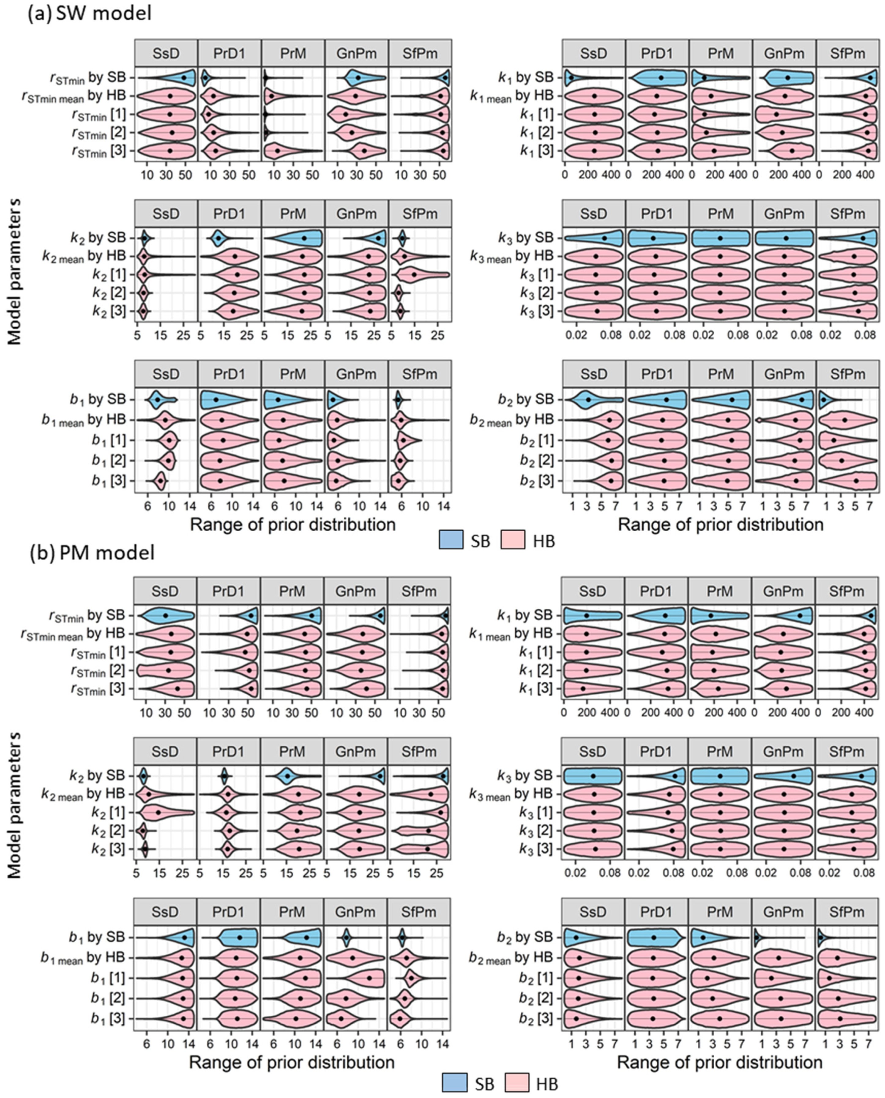
3.2.1. Comparison of Posterior Distributions of Model Parameters

A violin plot, depicting the posterior distribution of the SW and PM models parameters using the SB and HB approaches, is presented in Figure 3. The values of the posterior parameter distribution for the two models corresponding to the means and the 95% confidence intervals are given in Appendix B (

Table A1. Posterior probability distributions of the parameters in the Shuttleworth–Wallace (SW) and the Penman–Monteith (PM) models using simple Bayesian (SB) and hierarchical Bayesian (HB) approaches for five observations, characterized by the posterior means and 95% Bayesian confidence intervals.

Parameter	Model	Bayes	SsD	PrD1	PrM	GnPm	SfPm
rSTmin (s m−1)	SW	SB	45.8 (19.0, 59.5)	5.60 (1.60, 15.2)	2.10 (0.033, 10.4)	33.9 (19.6, 57.0)	54.4 (40.9, 59.8)
		HB	33.4 (5.40, 57.4)	15.8 (2.30, 45.2)	11.6 (0.41, 45.8)	29.4 (4.48, 55.8)	48.2 (19.1, 59.3)
	PM	SB	31.8 (9.46, 57.6)	52.0 (37.6, 59.7)	47.7 (22.3, 59.6)	54.3 (41.5, 59.8)	56.5 (47.7, 59.9)
		HB	35.2 (5.95, 57.6)	46.6 (16.4, 59.0)	40.9 (11.8, 58.4)	36.3 (8.55, 57.3)	51.2 (27.8, 59.4)
k1 (W m−2)	SW	SB	104 (2.10, 432)	284 (70.3, 489)	155 (2.30, 471)	286 (104, 488)	427 (266, 498)
		HB	256 (32.2, 473)	250 (37.4, 470)	185 (11.3, 453)	257 (36.3, 471)	381 (125, 492)
	PM	SB	214 (4.50, 483)	317 (86.1, 492)	197 (3.20, 479)	378 (177, 495)	446 (322, 498)
		HB	209 (14.4, 463)	309 (64.1, 483)	225 (22.9, 464)	254 (39.2, 470)	378 (137, 490)
k2 (°C)	SW	SB	8.41 (7.02, 10.6)	12.9 (10.0, 17.2)	21.6 (10.4, 29.6)	26.2 (18.8, 29.9)	9.70 (8.11, 11.0)
		HB	9.06 (5.55, 21.0)	19.7 (9.23, 28.6)	20.9 (8.76, 29.2)	22.0 (9.96, 29.3)	12.2 (5.82, 26.0)
	PM	SB	8.11 (6.66, 9.50)	15.7 (14.5, 17.0)	16.3 (10.95, 27.6)	27.2 (19.8, 29.9)	25.8 (11.6, 29.9)
		HB	12.0 (5.77, 26.0)	17.4 (10.2, 25.3)	20.1 (9.23, 28.9)	19.1 (8.34, 28.7)	21.5 (7.94, 29.5)
k3 (kPa−1)	SW	SB	0.063 (0.006, 0.099)	0.045 (0.002, 0.096)	0.049 (0.002, 0.097)	0.052 (0.003, 0.098)	0.069 (0.009, 0.099)
		HB	0.053 (0.006, 0.095)	0.048 (0.005, 0.094)	0.049 (0.005, 0.094)	0.050 (0.005, 0.095)	0.058 (0.008, 0.096)
	PM	SB	0.050 (0.003, 0.097)	0.077 (0.024, 0.099)	0.050 (0.002, 0.098)	0.063 (0.006, 0.099)	0.069 (0.009, 0.099)
		HB	0.052 (0.006, 0.095)	0.068 (0.015, 0.098)	0.051 (0.006, 0.095)	0.051 (0.005, 0.095)	0.056 (0.007, 0.096)
b1 (s m−1)	SW	SB	8.20 (6.39, 11.1)	7.26 (4.13, 12.0)	7.06 (4.12, 12.0)	5.21 (4.04, 7.36)	5.41 (4.92, 6.16)
		HB	9.42 (5.74, 13.2)	8.32 (4.45, 13.6)	8.00 (4.36, 13.6)	6.33 (4.16, 11.8)	6.22 (4.35, 10.6)
	PM	SB	12.9 (9.27, 14.9)	11.6 (8.13, 14.8)	12.0 (8.22, 14.9)	7.81 (7.07, 8.67)	6.29 (5.54, 7.05)
		HB	12.3 (7.03, 14.8)	10.9 (6.57, 14.5)	10.8 (5.61, 14.5)	9.06 (4.58, 14.2)	7.39 (4.49, 12.3)
b2 (s m−1)	SW	SB	3.65 (1.16, 7.66)	4.93 (0.626, 7.88)	5.18 (0.835, 7.89)	6.13 (2.86, 7.93)	0.774 (0.027, 2.33)
		HB	5.87 (2.23, 7.79)	4.54 (0.685, 7.67)	4.76 (0.789, 7.69)	5.19 (0.616, 7.78)	3.65 (0.40, 7.40)
	PM	SB	2.02 (0.072, 5.87)	3.59 (0.192, 6.96)	1.99 (0.069, 5.57)	0.419 (0.010, 1.55)	0.573 (0.013, 2.28)
		HB	2.43 (0.183, 6.55)	3.62 (0.359, 7.19)	3.30 (0.329, 7.19)	3.474 (0.315, 7.38)	2.98 (0.230, 7.17)
σ (mm day−1)	SW	SB	0.406 (0.348, 0.477)	0.702 (0.603, 0.821)	0.840 (0.723, 0.981)	0.509 (0.438, 0.595)	0.318 (0.273, 0.373)
		HB	0.310 (0.265, 0.364)	0.705 (0.604, 0.825)	0.806 (0.692, 0.943)	0.479 (0.412, 0.561)	0.285 (0.244, 0.336)
	PM	SB	1.20 (1.03, 1.40)	0.676 (0.581, 0.792)	0.948 (0.815, 1.11)	0.897 (0.768, 1.05)	1.05 (0.892, 1.23)
		HB	1.06 (0.911, 1.24)	0.646 (0.553, 0.760)	0.768 (0.660, 0.899)	0.701 (0.602, 0.820)	0.944 (0.808, 1.11)

).

These results showed that parameterizations using SB and HB were, in most cases, successful in reducing the uncertainties in the parameters. Several posterior distributions, such as the k₂ of SsD and the b₁ of SfPm for the SW model were strongly constrained, indicating their importance as a parameter for controlling ET estimation and partition (Figure 3a), as discussed below. In the estimation of the k₂ of SsD, we assumed that the strong correlation between T_a and the observed ET with the small LAI was a factor that constrained the posterior distributions, in order to reduce the value of T. SsD had the highest correlation with T_a and the observed ET of all crops. The correlation coefficients between daily T_a and the observed ET in descending order were SsD 0.66 > PrD1 0.57 > PrM 0.47 > GnPm 0.36 > SfPm 0.21. This strongly constrained k₂ of SsD at the low side of the prior bound indicated that the stomatal resistance of the canopy largely limited the value of T. In the estimation of the b₁ of SfPm in the SW model, the soil moisture of SfPm near the soil surface was the lowest of all observations (Figure 2). The posterior distribution range of b₁ associated with the soil surface resistance was, therefore, constrained to the low side of the prior range to reduce the value of E. The parameter k₃, which is related to D, was poorly constrained and displayed large variability in all observations (Figure 3). Although the D value differed considerably between the dry and monsoon seasons (Figure 2), there were no differences in the posterior distribution of k₃ between the two seasons for the SW model. As previous studies [17,18] showed, k₃ is an insensitive parameter of the models. Some parameters showed large differences between the SB and the HB on the posterior distribution. For example, the b₂ of SsD for the SB in the SW model was constrained at the low side on the prior bound, but that for the HB was restricted at the upper side, with no differences in group levels (Figure 3a). This observation indicated that the parameter b₂, calibrated by the SB and the HB, had different abilities under the same environmental factors, and thus might have made a difference in the estimated and partitioned ET between the SB and HB approaches (Figure 3a).

The range of posterior distributions for several parameters differed substantially between the SW and PM models. For example, the $r_{\mathrm{STmin}}$ of PrM of the SW model was well constrained compared to that of the PM model. For the PM model, the b₂ of SsD had lower uncertainty than that for the SW model. The differences in model structure between the SW and PM models affected the reduction in uncertainty in the parameter estimation. However, for most of the parameters and conditions, there were no large differences in the range of posterior distributions between the models.

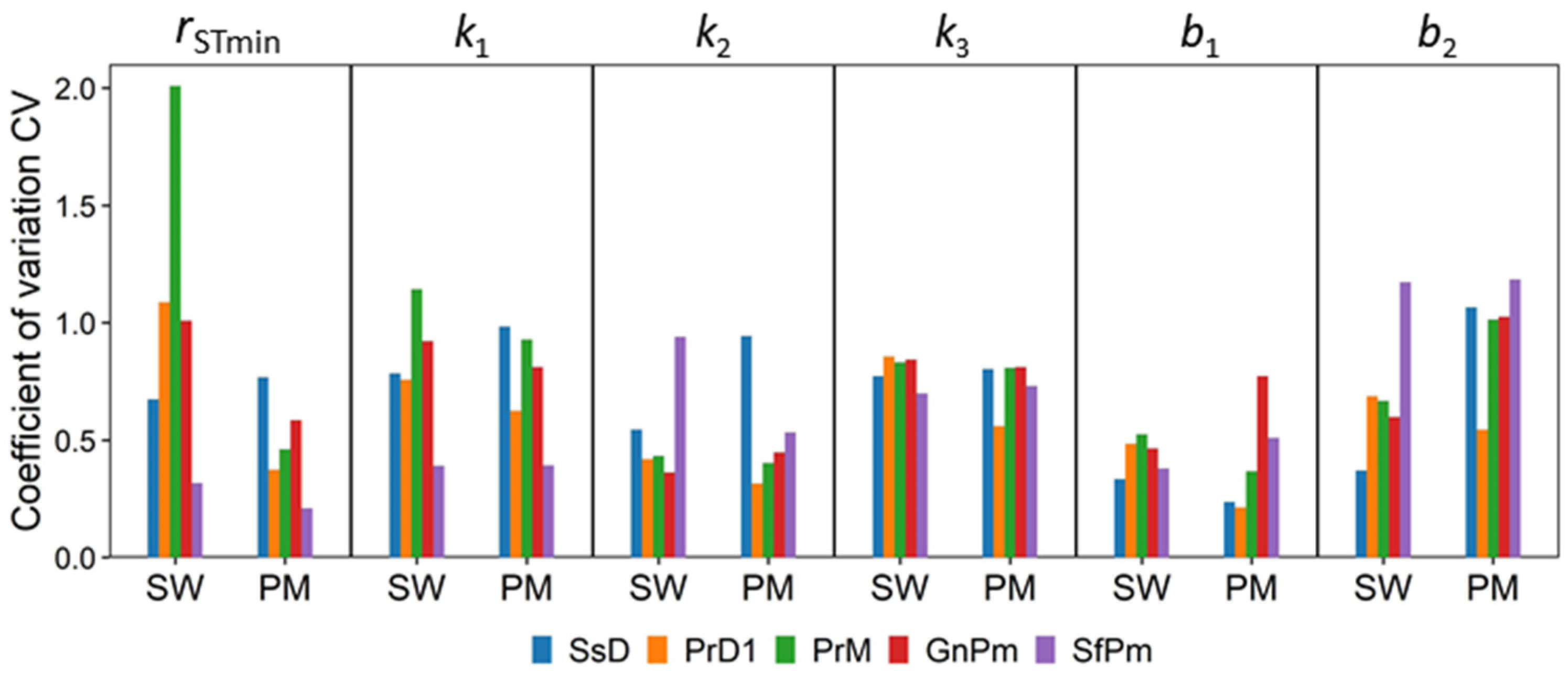
3.2.2. Effect of Difference in Observation Conditions on Parameter Estimation

The differences between the posterior distributions of the model parameters, estimated using the HB approach based on observed ET data over the three calibration periods, were clear in several cases (Figure 3), including the $r_{\mathrm{STmin}}$ of PrM and GnPm, the k₁ of GnPm, the k₂ of SfPm, and the b₁ of SsD in the SW model, and the k₂ of SsD and SfPm, the b₁ of GnPm, and the b₂ of SfPm in the PM model. However, in the k₃ of all conditions and all parameters for PrD1, these differences were unclear.

The degrees of variation in the posterior mean value of the three calibration periods in a dataset—the coefficient of variation (CV) for each parameter and observation—are shown in Figure 4. The CV was calculated from the posterior mean value of ${\sigma }_{{\theta }_s}$ divided by ${\theta }_{s,mean}$ in Equation (23). The CV values of $r_{\mathrm{STmin}}$, which are associated with stomatal resistance, varied greatly depending on the observations; the difference between the SW and PM models was also larger than those of other parameters. Since the two-layer SW model is sensitive to error in the values of canopy and soil resistance [10,43], measurement errors or improperly used constants and variables, such as K_a and LAI, may have increased the variation in the estimation of this parameter. In paddy fields, which have continuously saturated surfaces in which the fluctuations in the surface resistance are small, the variations in $r_{\mathrm{STmin}}$ may be strongly affected by the growth of the plant.

In contrast, the variability of k₃ was nearly constant, regardless of differences in the models and observations. The posterior distributions of k₃ were poorly constrained and widespread along prior ranges (Figure 3). As has been shown in previous studies [17,18,20], this observation suggests that k₃ is not very susceptible to seasonal fluctuations with large uncertainties. Therefore, k₃ may not be necessary for strict parameter estimation, and empirical values may suffice.

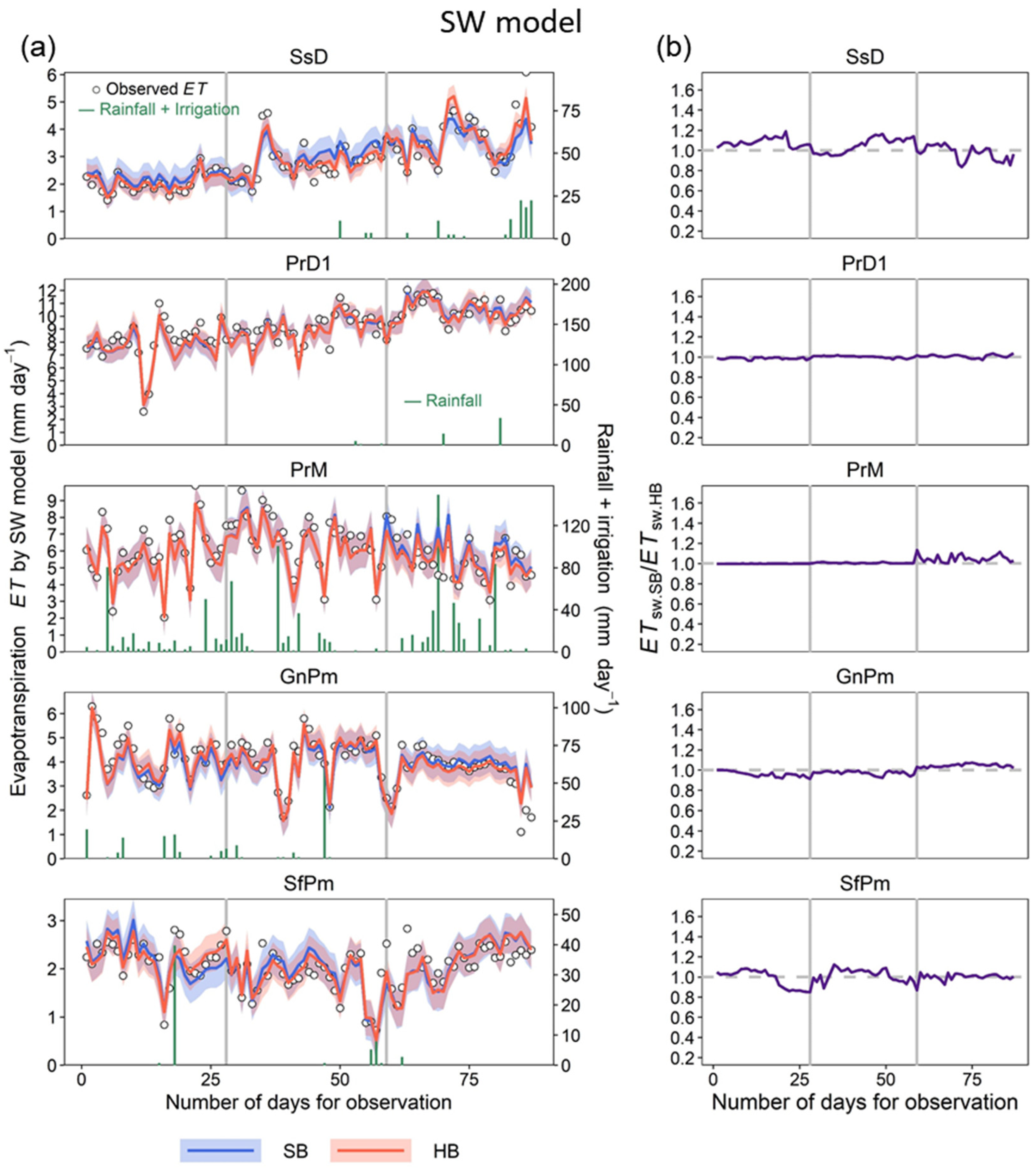
3.3. Comparison of ET Estimation by SW and PM Models Using SB and HB Approaches

Figure 5a and Figure 6a show the daily changes in observed and estimated ET using the SW and the PM models with parameters calibrated using the SB and HB approaches with irrigation + rainfall amount for SsD, while rainfall amount only was used for the others. Figure 5b and Figure 6b show the values corresponding to the difference in the SB and HB approaches on the estimated ET, calculated as the estimated ET of the SB approach divided by that of the HB approach. The ET observed and estimated by the two models with parameters calibrated by the SB and HB approaches with portioned E and T only for the SW model; the results of statistical evaluation for the model performances are shown in

Table 3. Observed and estimated evapotranspiration (ET) with partitioned evaporation (E) and transpiration (T) using the Shuttleworth–Wallace (SW) and the Penman–Monteith (PM) models with parameters calibrated using simple Bayesian (SB) and hierarchical Bayesian (HB) approaches, and statistical criteria under five observation conditions.

Model	Bayes Type	Condition	ETob (mm)	ETest (mm)	Eest (mm)	Test (mm)	MAE (mm d−1)	RMSE (mm d−1)	MAPE (%)	RMSPE (%)
SW	SB	SsD	248	253	182	71	0.275	0.388	0.099	0.120
		PrD1	798	783	110	673	0.562	0.684	0.065	0.087
		PrM	529	516	43	473	0.663	0.825	0.112	0.142
		GnPm	350	339	89	250	0.371	0.499	0.110	0.141
		SfPm	180	179	124	55	0.239	0.309	0.117	0.170
	HB	SsD	248	248	213	35	0.218	0.294	0.074	0.089
		PrD1	798	784	94	690	0.557	0.679	0.065	0.086
		PrM	529	506	43	463	0.642	0.786	0.106	0.140
		GnPm	350	342	78	264	0.341	0.464	0.103	0.133
		SfPm	180	179	129	49	0.205	0.272	0.102	0.153
PM	SB	SsD	248	217	–	–	0.921	1.17	0.333	1.37
		PrD1	798	796	–	–	0.529	0.657	0.062	0.077
		PrM	529	528	–	–	0.731	0.927	0.125	0.151
		GnPm	350	352	–	–	0.608	0.878	0.180	0.291
		SfPm	180	163	–	–	0.661	0.838	0.317	1.01
	HB	SsD	248	236	–	–	0.587	0.824	0.197	0.435
		PrD1	798	797	–	–	0.497	0.615	0.058	0.073
		PrM	529	527	–	–	0.597	0.737	0.102	0.126
		GnPm	350	355	–	–	0.484	0.675	0.147	0.177
		SfPm	180	163	–	–	0.535	0.669	0.266	0.627

Notes: ET_ob and ET_est indicate observed ET and estimated ET using the SW and PM models, respectively. E_est and T_est are the estimated E and T, respectively, using the SW model. MAE, mean absolute error; RMSE, root mean square error; MAPE, mean absolute percentage error; RMSPE, root mean square percentage error.

, and the regression analysis between the observed ET and that estimated by the models are presented in Figure 7.

For the SW model, generally, the posterior mean value of the parameters calibrated using the SB and HB approaches provided acceptable estimations of ET over 87 days (Figure 5a), and the differences in the estimated total values of ET between the SB and HB approaches were small: 0 to 1 mm for PrD1 and SfPm, and 3 to 10 mm for SsD, PrM, and GnPm (Table 3). However, for the PM model, there was a large difference between the estimated and observed ET, except for PrD1 and PrM (Figure 6a and Table 3). The confidence intervals of the posterior distributions on the estimated ET for the PM model were generally wider than those for the SW model, indicating that large uncertainty in the parameter values led to poor model performance. For the PrD1 of both models, the estimated total value of ET produced by the SB and HB approaches were very similar (Table 3). The values of ET_sw.SB/ET_sw.HB and ET_pm.SB/ET_pm.HB were close to 1.0 over the entire period (Figure 5b and Figure 6b), indicating a lack of variation in the posterior mean distributions at three calibration periods using the HB approach (Figure 3). The wc and LAI values changed constantly or linearly over all calibration periods (Figure 2). Therefore, even when the variables that affected the estimation of the parameters varied considerably over the calibration period, the variables would not have affected the parameter estimation for each period if the change ratio was a constant. For PrM with a small fluctuation in environmental factors, a slight difference in ET estimates between SB and HB was apparent in the third calibration period (Figure 5b and Figure 6b), possibly because the estimated LAI value varied in a different change rate at the third period (Figure 2). The averaged change rate of LAI for the three stages in PrM were 3.2%, 1.0%, and 0.1%. For SsD and SfPm, large fluctuations in environmental factors produced differences between the ET estimates obtained using the SB and HB approaches for almost the entire period, especially in the PM model (Figure 5 and Figure 6). This observation suggests that the SW model could adapt well to changes in seasons and surface conditions with respect to parameter estimation, but the PM model was subject to environmental fluctuation in the calibration period.

The ET estimates obtained using the HB approach in both models were better than those produced using the SB approach in both models, indicating that the performance of the SW model was superior to that of the PM model (Table 3). The slope of the estimates obtained using the HB approach in the regression was closer to 1 than that produced by the SB for most observation conditions in both models (Figure 7). Considering the magnitude of errors for the BREB method, which are reported to be in order from several to 10 percent (e.g., [44]), it is not appropriate to evaluate the accuracy of estimated ET with parameters calibrated using the SB and HB approaches. However, the HB approach improved the fit of the model to the observed data, indicating the potential importance of accounting for seasonal fluctuations and variations in crop growth stages in calibrating models which can reliably predict ET.

For ET partitioning in PrM for the SB and HB approaches in the SW model (Table 3), the E_est and E_est/ET_est values were very small, at 43 mm and 0.08, respectively, indicating the improper use of estimated LAI values, or the uncertainty in ET partitioning by the SW model calibrated using only observed ET data. However, due to the lack of direct measurements of the different components of ET, it is not possible to validate the partitioned ET values using the SB and HB approaches in the SW model, although the estimated total ET was acceptable. Thus, multiple observations obtained using lysimeters and measures of sap flow should be used to validate ET partitioning into E and T by the SW model using the Bayesian approach in future studies.

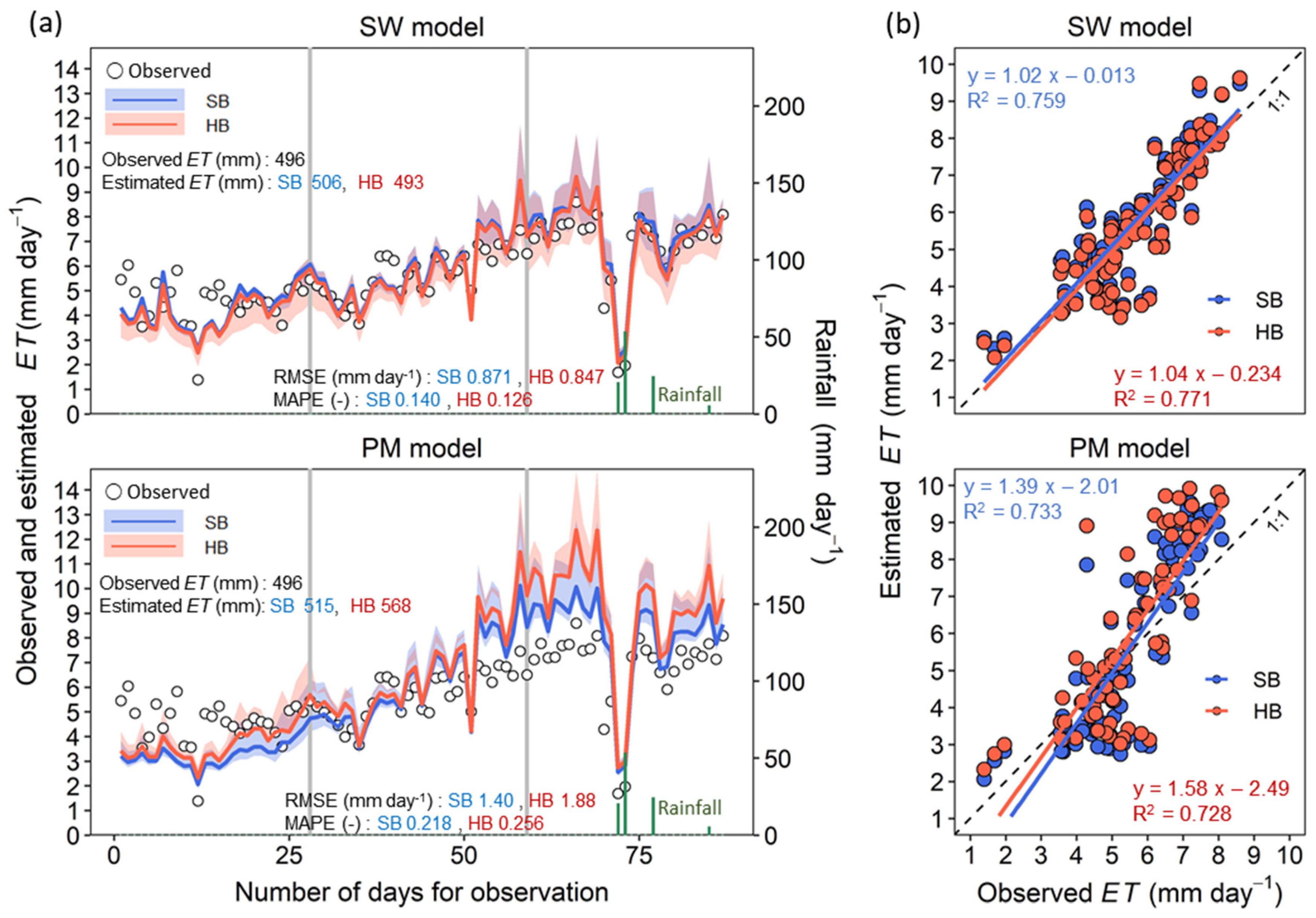
3.4. Validation of Model ET Estimation

Applying the posterior mean values of the parameters generated by the SB and the HB approaches using the dataset of PrD1 (Table A1), the model performance of the SW and the PM models were validated using the dataset of PrD2, as shown in Figure 8.

The ET estimates of the SW model were approximately equal to the observed ET, except during the initial stage, and there were few differences in the estimated ET using parameters calibrated by the SB and the HB approaches. The PM model overestimated ET in the last half period; the estimated ET using parameters obtained using the HB approach was slightly larger than those obtained using the SB approach.

Numerous studies have shown that the two-layer SW model has higher performance for ET estimation than other ET models, a finding consistent with those of our study. These studies have confirmed that the differences in the model structure by which ET is partitioned into E and T is related to the model performance (e.g., [16,17,45,46,47,48]). The ET estimation of the SW model with parameters calibrated using the Bayesian approaches was acceptable for the paddy field condition, suggesting the usefulness of the two-layer SW model. The low level of difference between the SB and HB approaches in the ET estimation of the SW model may be related to the small environmental fluctuations in the calibration period (PrD1).

The overestimation of ET by the PM model in this study agrees with the results of several previous studies (e.g., [9,48]), but some studies have found that the difference between the SW and PM models is not significant [8,49]. Generally, the performance of ET model is strongly related to the surface resistance, which is calculated as the integration of the canopy and soil surface resistances and reflects the effects of soil moisture and variation in LAI [50]. Some studies (e.g., [46]) reported that when the surface resistance in the PM model is lower than the observed resistance, the PM model overestimates ET. Thus, this overestimation in this study indicates an inadequate parameter estimation of the surface resistance, affected by the model structure of the PM model. The estimated mean value of $r_{\mathrm{s}}^{\mathrm{c}}$ in the PM model using the parameters from the HB approach was slightly lower (54 m s⁻¹) than that from the SB approach (69 m s⁻¹) during the last half period. The posterior means of $r_{\mathrm{STmin}}$ for PrD1 generated by the SB and HB approaches were 52 m s⁻¹ and 47 m s⁻¹, respectively, and those of other parameters also differed slightly between the SB and HB approaches (Table A1). Since the validation was performed using only the dataset of the paddy field conditions, the validity of the HB approach must be further verified using calibration data including large seasonal fluctuations and variations in crop growth.

4. Conclusions

In this study, we assessed the estimation of ET and the parameters of the SW and PM models calibrated using SB and HB approaches, based on a field-based ET dataset collected from five agricultural fields over three seasons in Myanmar. The main conclusions were as follows:

• Parameterization using the SB and HB approaches was, in most cases, successful in reducing the uncertainties in the parameters. Using the HB approach to parameter estimation, we identified the parameters which are sensitive to seasonal fluctuations and differences in crop growth stages. The parameter k₃, which is related to the water vapor pressure deficit, was not very susceptible to seasonal fluctuations, while r_STmin, which is related to stomatal resistance, was sensitive to variations in observation conditions.
• In the calibration of model parameters, the statistical criteria for all conditions observed indicated that the models with parameters calibrated using the HB approach had a better fit to the observed ET data than those with parameters calculated using the SB approach, indicating the potential importance of seasonal fluctuations and variability in crop growth stages for the calibration of model parameters. The performance of the SW models was superior to that of the PM model for most of the observation conditions, using both the SB and HB approaches.
• The SW model, with parameters calculated using the SB and HB approaches with only observed ET data, could provide an acceptable estimation of the ET. The PM model with parameters calculated using both SB and HB approaches overestimated the ET in the last half period; the ET estimates for the HB approach were slightly overestimated compared with the SB approach.

References

1. Flumignan, D.L.; Faria, R.T.; Prete, C.E.C. Evapotranspiration components and dual crop coefficients of coffee trees during crop production. Agric. Water Manag. 2011, 98, 791–800. [Google Scholar] [CrossRef]
2. Williams, D.G.; Cable, W.; Hultine, K.; Hoedjes, J.C.B.; Yepez, E.A.; Simonneaux, V.; Er-Raki, S.; Boulet, G.; de Bruin, H.A.R.; Chehbouni, A.; et al. Evapotranspiration components determined by stable isotope, sap flow and eddy covariance techniques. Agric. For. Meteorol. 2004, 125, 241–258. [Google Scholar] [CrossRef]
3. Moran, M.S.; Scott, R.L.; Keefer, T.O.; Emmerich, W.E.; Hernandez, M.; Nearing, G.S.; Paige, G.B.; Cosh, M.H.; O’Neill, P.E. Partitioning evapotranspiration in semiarid grassland and shrubland ecosystems using time series of soil surface temperature. Agric. For. Meteorol. 2009, 149, 59–72. [Google Scholar] [CrossRef]
4. Monteith, J.L. Evaporation and environment. In Symposia of the Society for Experimental Biology; Cambridge University Press (CUP): Cambridge, UK, 1965; Volume 19, pp. 205–234. [Google Scholar]
5. Anadranistakis, M.; Liakatas, A.; Kerkides, P.; Rizos, S.; Gavanosis, J.; Poulovassilis, A. Crop water requirements model tested for crops grown in Greece. Agric. Water Manag. 2000, 45, 297–316. [Google Scholar] [CrossRef]
6. Gardiol, J.M.; Serio, L.A.; Maggiora, A.D. Modelling evapotranspiration of corn (Zea mays) under different plant densities. J. Hydrol. 2003, 271, 188–196. [Google Scholar] [CrossRef]
7. Kato, T.; Kimura, R.; Kamichika, M. Estimation of evapotranspiration, transpiration ratio and water-use efficiency from a sparse canopy using a compartment model. Agric. Water Manag. 2004, 65, 173–191. [Google Scholar] [CrossRef]
8. Fisher, J.B.; Debiase, T.A.; Qi, Y.; Xu, M.; Goldstein, A.H. Evapotranspiration models compared on a Sierra Nevada forest ecosystem. Environ. Model. Softw. 2005, 20, 783–796. [Google Scholar] [CrossRef] [Green Version]
9. Zhou, M.; Ishidaira, H.; Hapuarachchi, H.; Magome, J.; Kiem, A.; Takeuchi, K. Estimating potential evapotranspiration using Shuttleworth–Wallace model and NOAA-AVHRR NDVI data to feed a distributed hydrological model over the Mekong River basin. J. Hydrol. 2006, 327, 151–173. [Google Scholar] [CrossRef]
10. Ortega-Farias, S.; Carrasco, M.; Olioso, A.; Acevedo, C.; Poblete, C. Latent heat flux over Cabernet Sauvignon vineyard using the Shuttleworth and Wallace model. Irrig. Sci. 2007, 25, 161–170. [Google Scholar] [CrossRef]
11. Shuttleworth, W.J.; Wallace, J.S. Evaporation from sparse crops—An energy combination theory. Q. J. R. Meteorol. Soc. 1985, 111, 839–855. [Google Scholar] [CrossRef]
12. Kool, D.; Agam, N.; Lazarovitch, N.; Heitman, J.L.; Sauer, T.J.; Ben-Gal, A. A review of approaches for evapotranspiration partitioning. Agric. For. Meteorol. 2014, 184, 56–70. [Google Scholar] [CrossRef]
13. Samanta, S.; Mackay, D.S.; Clayton, M.K.; Kruger, E.L.; Ewers, B.E. Bayesian analysis for uncertainty estimation of a canopy transpiration model. Water Resour. Res. 2007, 43. [Google Scholar] [CrossRef]
14. Reinds, G.J.; van Oijen, M.; Heuvelink, G.B.M.; Kros, H. Bayesian calibration of the VSD soil acidification model using European forest. Geoderma 2008, 146, 475–488. [Google Scholar] [CrossRef] [Green Version]
15. Finsterle, S.; Najita, J. Robust estimation of hydrologic model parameters. Water Resour. Res. 1998, 34, 2939–2947. [Google Scholar] [CrossRef] [Green Version]
16. Zhu, G.F.; Su, Y.H.; Li, X.; Zhang, K.; Li, C.B. Estimating actual evapotranspiration from an alpine grassland on Qinghai–Tibetan plateau using a two-source model and parameter uncertainty analysis by Bayesian approach. J. Hydrol. 2013, 476, 42–51. [Google Scholar] [CrossRef]
17. Zhu, G.F.; Li, X.; Su, Y.H.; Zhang, K.; Bai, Y.; Ma, J.Z.; Li, C.B.; Hu, X.L.; He, J.H. Simultaneously assimilating multivariate data sets into the two-source evapotranspiration model by Bayesian approach: Application to spring maize in an arid region of northwestern China. Geosci. Model Dev. 2014, 7, 1467–1482. [Google Scholar] [CrossRef] [Green Version]
18. Wei, G.; Zhang, X.; Ye, M.; Yue, N.; Kan, F. Bayesian performance evaluation of evapotranspiration models based on eddy covariance systems in an arid region. Hydrol. Earth Syst. Sci. 2019, 23, 2877–2895. [Google Scholar] [CrossRef] [Green Version]
19. Chen, D.Y.; Wang, X.; Liu, S.Y.; Wang, Y.K.; Gao, Z.Y.; Zhang, L.L.; Wei, X.G.; Wei, X.D. Using Bayesian analysis to compare the performance of three evapotranspiration models for rainfed jujube (Ziziphus jujuba Mill) plantations in the Loess Plateau. Agric. Water Manag. 2015, 159, 341–357. [Google Scholar] [CrossRef]
20. Song, Y.; Jin, L.; Zhu, G.; Ma, M. Parameter estimation for a simple two-source evapotranspiration model using Bayesian inference and its application to remotely sensed estimations of latent heat flux at the regional scale. Agric. For. Meteorol. 2016, 230–231, 20–32. [Google Scholar] [CrossRef]
21. Clark, J.S.; Gelfand, A.E. Hierarchical Modelling for the Environmental Sciences. In Statistical Methods and Applications; Oxford University Press: Oxford, UK, 2006. [Google Scholar]
22. Nilsson, H.; Rieskamp, J.; Wagenmakers, E. Hierarchical Bayesian parameter estimation for cumulative prospect theory. J. Math. Psychol. 2011, 55, 84–93. [Google Scholar] [CrossRef]
23. Morey, R.D.; Pratte, M.S.; Rouder, J.N. Problematic effects of aggregation in z ROC analysis and a hierarchical modeling solution. J. Math. Psychol. 2008, 52, 376–388. [Google Scholar] [CrossRef]
24. Bowen, I.S. The ratio of heat losses by conduction and by evaporation from any water surface. Phys. Rev. 1926, 27, 779–787. [Google Scholar] [CrossRef] [Green Version]
25. Weine, N.N.O. Review of Efforts to Combat Desertification and Arrest and Reverse Land Degradation in Myanmar. In Combating Desertification in Asia, Africa and the Middle East; Heshmati, G., Squires, V., Eds.; Springer: Dordrecht, The Netherlands, 2013. [Google Scholar] [CrossRef]
26. Casanova, D.; Epema, G.F.; Goudriaan, J. Monitoring rice reflectance at field level for estimating biomass and LAI. Field Crop. Res. 1998, 55, 83–92. [Google Scholar] [CrossRef]
27. Allen, R.G.; Jensen, M.E.; Wright, J.L.; Burman, R.D. Operational Estimates of Reference Evapotranspiration. Agron. J. 1989, 81, 650. [Google Scholar] [CrossRef]
28. Kim, S.; Kim, H.S. Neural networks and genetic algorithm approach for nonlinear evaporation and evapotranspiration modeling. J. Hydrol. 2008, 351, 299–317. [Google Scholar] [CrossRef]
29. Shibayama, M.; Sakamoto, T.; Takada, E.; Inoue, A.; Morita, K.; Takahashi, W.; Kimura, A. Estimating Paddy Rice Leaf Area Index with Fixed Point Continuous Observation of Near Infrared Reflectance Using a Calibrated Digital Camera. Plant Prod. Sci. 2011, 14, 30–46. [Google Scholar] [CrossRef] [Green Version]
30. Wei, Z.; Lee, X.; Wen, X.; Xiao, W. Evapotranspiration partitioning for three agro-ecosystems with contrasting moisture conditions: A comparison of an isotope method and a two-source model calculation. Agric. For. Meteorol. 2018, 252, 296–310. [Google Scholar] [CrossRef]
31. Kar, G.; Kumar, A. Surface energy fluxes and crop water stress index in groundnut under irrigated ecosystem. Agric. For. Meteorol. 2007, 146, 94–106. [Google Scholar] [CrossRef]
32. Banik, C.N.; Nath, R.; Chakraborty, P.K. Effect of dates of sowing on growth and yield of groundnut crop. J. Crop. Weed. 2009, 5, 59–62. [Google Scholar]
33. Chapman, S.C.; Hammer, G.L.; Palta, J.A. Predicting leaf area development of sunflower. Field Crop. Res. 1993, 34, 101–112. [Google Scholar] [CrossRef]
34. Chongdar, S.; Singharoy, A.; Saha, A.; Chhetri, B. Performance of summer sesame (Sesamum indicum L.) cultivars under varying dates of sowing in prevailing agro-climatic condition of North Bengal. Sci. Res. Essays 2015, 10, 411–420. [Google Scholar] [CrossRef]
35. Shuttleworth, W.J.; Gurney, R.J. The theoretical relationship between foliage temperature and canopy resistance in sparse crops. Q. J. R. Meteorol. Soc. 1990, 116, 497–519. [Google Scholar] [CrossRef]
36. Jarvis, P.G. The interpretation of the variations in leaf water potential and stomatal conductance found in canopies in the field. Philos. Trans. R. Soc. B Biol. Sci. 1976, 273, 593–610. [Google Scholar] [CrossRef]
37. Stewart, J.B. Modelling surface conductance of pine forest. Agric. For. Meteorol. 1988, 43, 19–35. [Google Scholar] [CrossRef]
38. Li, S.; Kang, S.; Zhang, L.; Ortega-Farias, S.; Li, F.; Du, T.; Tong, L.; Wang, S.; Ingman, M.; Guo, W. Measuring and modeling maize evapotranspiration under plastic film-mulching condition. J. Hydrol. 2013, 503, 153–168. [Google Scholar] [CrossRef]
39. Stewart, G.H. The influence of canopy cover on understorey development in forests of the western Cascade Range, Oregon, USA. Vegetatio 1988, 76, 79–88. [Google Scholar] [CrossRef]
40. Brutsaert, W. Theory, History, and Applications. In Evaporation into the Atmosphere; Reidel: Dordrecht, The Netherlands, 1982; p. 299. [Google Scholar]
41. Stan Modelling Language Users Guide and Reference Manual, Version 2.4. Available online: http://mc-stan.org/rstan (accessed on 23 October 2020).
42. Sellers, P.J.; Heiser, M.D.; Hall, F.G. Relations between surface conductance and spectral vegetation indices at intermediate (100 m2 to 15 km2) length scales. J. Geophys. Res. 1992, 97, 19033–19059. [Google Scholar] [CrossRef] [Green Version]
43. Meng, W.; Xihuan, S.; Juanjuan, M.; Xianghong, G.; Tao, L.; Ruofan, L. Measurement and simulation of the water storage pit irrigation trees evapotranspiration in the Loess Plateau. Agric. Water Manag. 2019, 226, 105804. [Google Scholar] [CrossRef]
44. Gavilán, P.; Berengena, J. Accuracy of Bowen ratio-energy balance method for measuring latent heat flux in a semiarid advective environment. Irrig. Sci. 2007, 25, 127–140. [Google Scholar] [CrossRef]
45. Ershadi, A.; McCabe, M.F.; Evans, J.P.; Wood, E.F. Impact of model structure and parameterization on Penman–Monteith type evaporation models. J. Hydrol. 2015, 525, 521–535. [Google Scholar] [CrossRef] [Green Version]
46. Stannard, D.I. Comparison of Penman-Monteith, Shuttleworth-Wallace, and Modified Priestley-Taylor Evapotranspiration Models for wildland vegetation in semiarid rangeland. Water Resour. Res. 1993, 29, 1379–1392. [Google Scholar] [CrossRef]
47. The, C.B.S.; Simmonds, L.P.; Wheeler, T.R. Modelling the partitioning of solar radiation capture and evapotranspiration intercropping systems. In Proceedings of the 2nd International Conference on Tropical Climatology, Meteorology and Hydrology TCMH-2001, Brussels, Belgium, 13–14 December 2001. [Google Scholar]
48. Zhang, B.; Kang, S.; Li, F.; Zhang, L. Comparison of three evapotranspiration models to Bowen ratio-energy balance method for a vineyard in an arid desert region of northwest China. Agric. For. Meteorol. 2008, 148, 1629–1640. [Google Scholar] [CrossRef]
49. Ortega-Farias, S.O.; Olioso, A.; Fuentes, S.; Valdes, H. Latent heat flux over a furrow-irrigated tomato crop using Penman–Monteith equation with a variable surface canopy resistance. Agric. Water Manag. 2006, 82, 421–432. [Google Scholar] [CrossRef]
50. Burba, G.G.; Verma, S.B. Seasonal and interannual variability in evapotranspiration of native tallgrass prairie and cultivated wheat ecosystems. Agric. For. Meteorol. 2005, 135, 190–201. [Google Scholar] [CrossRef]
51. Alves, I.; Cameira, M. Evapotranspiration estimation performance of root zone water quality model: Evaluation and improvement. Agric. Water Manag. 2002, 57, 61–73. [Google Scholar] [CrossRef]
52. Denmead, O.T. Temperate Cereals. In Vegetation and the Atmosphere; Monteith, J.L., Ed.; Academic Press: New York, NY, USA, 1976; Volume 2, pp. 1–31. [Google Scholar]
53. Uchijima, Z. Maize and rice. In Vegetation and the Atmosphere; Monteith, J.L., Ed.; Academic Press: New York, NY, USA, 1976; Volume 2, pp. 33–64. [Google Scholar]
54. Monteith, J.L. Principles of Environmental Physics; Edward Arnold: London, UK, 1973; p. 241. [Google Scholar]
Figure 1. (a) Study site location and (b) experimental fields where evapotranspiration was observed.
Water 13 03607 g001
Figure 2. Variations in daily net radiation (Rn), air temperature (Ta), air water vapor pressure deficit (D), wind speed (U), soil moisture content (wc), and plant height (hc) with estimated leaf area index (LAI) in different observation periods at three fields in the dry season, a different field in the monsoon season, and a third set of two fields in the post-monsoon season. The three calibration periods for HB are indicated by vertical lines.
Water 13 03607 g002
Figure 3. Violin plots of the posterior distributions of (a) the Shuttleworth–Wallace (SW) and (b) the Penman–Monteith (PM) model parameters calibrated using simple Bayesian (SB) and hierarchical Bayesian (HB) approaches. The numbers in square brackets with parameters indicate the three calibration periods of the HB approach. Parameters with mean by HB represent the overall mean distribution. The black dotted circles and horizontal lines inside the violin shapes represent the posterior means and 95% confidence intervals.
Water 13 03607 g003
Figure 4. Coefficient of variation of posterior mean values of the parameters estimated in the Shuttleworth–Wallace (SW) and Penman–Monteith (PM) models using the hierarchical Bayesian (HB) approach, calculated from σ θ s divided by θ s , m e a n in Equation (23), indicating the degree of variation in the posterior mean value of the three calibration periods.
Water 13 03607 g004
Figure 5. (a) Observed and estimated evapotranspiration (ET) using the Shuttleworth–Wallace (SW) model with parameters calibrated using simple Bayesian (SB) and hierarchical Bayesian (HB) approaches. Lines and bands corresponding to the posterior means and confidence intervals at the 95% probability, respectively, in all five observation conditions. Vertical bars indicate the rainfall + irrigation amount for the SsD and rainfall only for the others. (b) Variations in the values of ETsw.SB and ETsw.HB calculated from ET estimates by the SW model using SB and HB. The three calibration periods for HB are separated by vertical lines.
Water 13 03607 g005
Figure 6. (a) Observed and estimated evapotranspiration (ET) using the Penman–Monteith (PM) model with parameters calibrated using the simple Bayesian (SB) and hierarchical Bayesian (HB) approaches. Lines and bands correspond to the posterior means and confidence intervals at the 95% probability, respectively, in all five observation conditions. Vertical bars indicate the rainfall + irrigation amount for the SsD and rainfall only for the others. (b) Variations in the values of ETpm.SB and ETpm.HB calculated from ET estimates by the PM model using SB and HB. The three calibration periods for HB are separated by vertical lines.
Water 13 03607 g006
Figure 7. Regression analysis of observed and estimated evapotranspiration (ET) produced by (a) the Shuttleworth–Wallace (SW) and (b) the Penman–Monteith (PM) models with parameters calibrated using simple Bayesian (SB) and hierarchical Bayesian (HB) approaches at five observation conditions. R2, coefficient of determination.
Water 13 03607 g007
Figure 8. (a) Comparison of observed evapotranspiration (ET) for the paddy rice field in the dry season of 2017 (PrD2) and estimated ET produced by the Shuttleworth–Wallace (SW) and the Penman–Monteith (PM) models with calibrated parameters using the simple Bayesian (SB) and hierarchical Bayesian (HB) approaches for the paddy rice field in the dry season of 2019 (PrD1). Lines and bands indicate the mean values and 95% confidence intervals of the estimated ET. (b) Regression analysis of estimated ET calculated by the SW and the PM models using calibrated parameters of PrD1 with observed ET of PrD1. RMSE, root mean square error; MAPE, mean absolute percentage error; R2, coefficient of determination.
Water 13 03607 g008