Article

Evolution of Surface Drainage Network for Spoil Heaps under Simulated Rainfall

1
Key Laboratory of Mountain Surface Processes and Ecological Regulation, Institute of Mountain Hazards and Environment, Chinese Academy of Sciences, Chengdu 610000, China
2
Institute of Soil and Water Conservation, Northwest A&F University, Yangling 712100, China
*
Authors to whom correspondence should be addressed.
Water 2021, 13(23), 3475; https://doi.org/10.3390/w13233475
Submission received: 27 October 2021 / Revised: 22 November 2021 / Accepted: 1 December 2021 / Published: 6 December 2021
(This article belongs to the Special Issue Latest Advances in Urban Stormwater Pollution Management)

Abstract

:
Spoil heaps laid from the infrastructure building sites or the mining sites are confoundedly prone to accelerated soil erosion and inducing debris flows on extreme rainfall occasion, thus threatening water quality and personal safety. In present study, the roughness and drainage network evolution of the loess spoil heap (a 33° slope gradient) were investigated via indoor simulation experiment under three rainfall intensities (60, 90, and 120 mm/h). A detailed scan of the slope using laser scanner, topographic analysis based on ArcGIS software, and statistical analyses were the main methods utilized in the study. The results showed that surface roughness increased with cumulative rainfall. For three rainfall intensity treatments, the proneness of shallow landslide under 90 mm/h intensity resulted in the largest roughness. The drainage density and stream frequency of the spoil heap slope both decreased with cumulative rainfall and negatively correlated with surface roughness, which indicated the convergence of the drainage network. Meanwhile, the individual flow paths presented an increasing sinuosity and a decreasing gradient with cumulative rainfall. However, drainage network features varied in a less marked degree during different rainfall intensities, showing comparable fractal dimensions of 1.350–1.454, 1.305–1.459, and 1.292–1.455 for the three rainfall intensities. Evaluating the response of four hydrodynamic characteristics of runoff to the drainage network evolution, stream power was found to be most sensitive. The linearity of the relationships between stream power and drainage density and that between stream sinuosity and gradient were estimated to have R2 between 0.961 and 0.979.

1. Introduction

The extensive development of urbanization has resulted in a dramatic increase in construction waste in recent years. Spoil heaps exist widely on infrastructure building sites or the mining sites, with characteristics of multiple porosity, weak consolidation, and steep slope [1,2,3,4]. In the last years, intense erosion acceleration of spoil heaps has received increasing attention [5,6], including the disasters on spoil heaps, such as debris flows and landslide on extreme rainfall occasion [7]. The eroded sediments threaten water quality and the safety of life and property [3,8,9,10].
Rainfall and overland flow induce erosion and sediment transport. The process-based erosion prediction models, like WEPP and EUROSEM, for instance, adopt hydrodynamic parameters of overland flow to simulate rill and inter-rill erosion of slopes [11,12]. Such attempts were based on a formed terrain with distinct rill and inter-rill area, and the hydraulic features of overland flow can be determined clearly. However, in many cases, surface morphology of slopes developed gradually in erosion process and led to corresponding evolution of drainage network as well as rill development [13]. Thus, the adaptability of hydrodynamic parameters to drainage network changes still needs to be considered.
High-precision laser scanning and digital photogrammetry have enabled the subtle study of surface roughness and drainage networks of slope [14,15]. The drainage networks have a degree of similarity and regularity, and the river principle on a river-basin scale has been applied on a slope scale in some research [16]. Helming et al. [17] also confirmed that drainage networks on eroding surfaces (flume scale) were similar to those of river systems. Based on the theory of river geomorphology [18], some researchers have extracted the drainage networks of cultivated slope to analyze the convergence levels, density, and extending direction of the drainage [19,20]. In addition, surface roughness was supposed to influence overland flow on flow direction and pattern markedly. Gómez et al. [21] studied the relationship between roughness levels and drainage network orientation, showing that the effect of the initial microrelief dominated the network structure, and the drainage density evolved most clearly for low roughness. Results of Luo et al. [20] confirmed that increasing microrelief had a considerable hindering effect on the evolution of drainage networks on a ridge tillage landform. These studies are aimed at agricultural land with gently sloping tillage surfaces (less than 15°), and very few similar studies have been reported for steep slopes, such as spoil heaps.
Since spoil heap is liable to be eroded because of the weak consolidation and steep slope, the topographical development is more intense than other soil surfaces, especially gravitational erosion, which happens occasionally [22]. Consequently, flow paths in the inter-rill area converge to intensify the incision force, promoting the rills to take shape more rapidly [19,21,23]. However, few studies have focused on the evolution of drainage network development and its influence on hydraulic features on spoil heap slopes.
In the present study, an indoor simulation experiment was conducted with a loess spoil heap (with a 33° slope gradient) under three rainfall intensities (60, 90, and 120 mm/h). The surface topography of the spoil heap was captured by a laser scanner during four successive simulated rainfalls. The drainage network and surface roughness were extracted aided by DEM analysis to investigate the evolution and the relationship between them in rainfall sequence. What is more, the effect of drainage network characteristics on the runoff hydrodynamic parameters was also studied.

2. Materials and Methods

2.1. Materials

Spoil heaps are often a mixture of soil and rock fragments [4]. The soil and rock fragments used in the experiment were collected from spoil heaps in a construction area around Yangling, Xianyang, Shanxi. The soil was passed through a 10-mm sieve to remove debris. The soil mechanical composition was 27.6% clay, 48.2% silt, and 23.3% sand. According to the classification of the IUSS Working Group WRB [24], the soil belonged to the urbic technosol group. The rock fragments were siliceous limestone with diameters from 1 to 15 cm, classified into four categories by size: 1–3.5 cm, 3.5–7 cm, 7–10 cm, and 10–15 cm. Based on the composition of local landslide rock fragments, the classification groups were at a ratio of 2:3:3:2, respectively, and then mixed with the soil to simulate spoil heap materials.

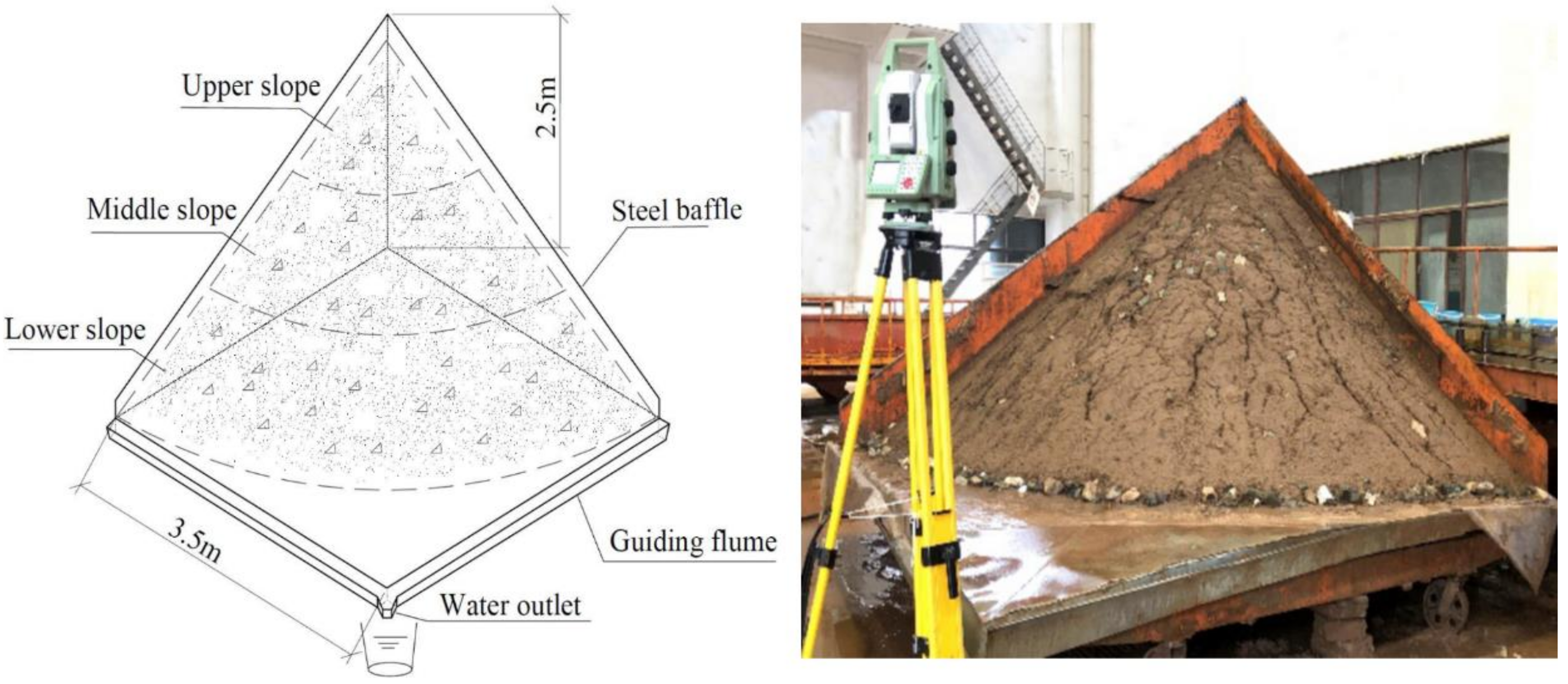
2.2. Spoil Heap Simulation

The experiment was conducted at rainfall simulation laboratory of the State Key Laboratory of Soil Erosion and Dryland Farming on the Loess Plateau, Yangling City, China. The rainfall simulation system was produced from many rotating sprinkler rainfall simulator, which is made of pressure pipes attached to nozzles. The pressure pipes and nozzles are arranged on a plot bed at a height of 18 m on the ceiling of the laboratory. The height ensures that the droplet diameters and distribution were similar to those of natural rainfall (rainfall uniformity over 80%). The effective rainfall area of the experiment area is 27 m × 18 m. The rainfall simulator can simulate rainfall intensities ranging from 30 to 350 mm/h by adjusting the pipe pressure and the nozzle size on a computing control terminal [25].
A square steel platform 3.5 m × 3.5 m connected two triangular baffles 2.5-m high to form the simulation device (Figure 1). The guiding flumes on the edges of the platform, which was inclined at 5°, allowed runoff to discharge at the outlet. The platform was inclined 3° to the water outlet for the same purpose. Gauzes were attached to the inside of the triangular baffles to reduce the boundary effect of the interface between soil and the baffles.
To simulate the formation of spoil heaps, a conveyor belt was first used to transfer the spoil heap materials to a position 2.8 m above the platform. Then, the soil was dumped to form a pile naturally under gravity. Finally, a quarter of the conical spoil heap was made with a bottom radius of 3.5 m. The slope length was 4.2 m, and the slope gradient was the angle of natural repose (in this case 33° ± 1°). These dimensions reflect the field survey data in the study area, in which it was reported that for more than 80% of the spoil heaps being investigated, slope lengths were 2.5–5.5 m, and gradients were 27°–36° [4].

2.3. Experimental Procedure

Each experiment consisted of four consecutive rainfall simulations 24 h apart, with a constant rainfall intensity. Three simulated rainfall intensities of 60, 90, and 120 mm/h were designed (rectangular distribution) to be similar to the local rainfall recorded over many years, which was concentrated in summer and autumn [26]. Each experiment was repeated three times.
Rainfall intensity was monitored before each rainfall simulation using five rain gauges located on the flume edges to ensure that the rainfall intensities remained stable (coefficient of variation 5%). The duration of each rainfall event was 60, 40, and 30 min for 60, 90, and 120 mm/h intensity, respectively, to ensure consistent simulated precipitation in each experiment. Runoff samples were taken every minute for the first 4 min and every 2 min thereafter to enable calculation of the runoff yield in the rainfall event.
Three 1-m long sections were set within a distance of 0.5–3.5 m from the top of the slope (Figure 1). A tracer dye (KMnO4) was used to time the runoff passing through each section for every runoff sample. The average velocity of the three sections was adopted as the runoff velocity on the entire slope.

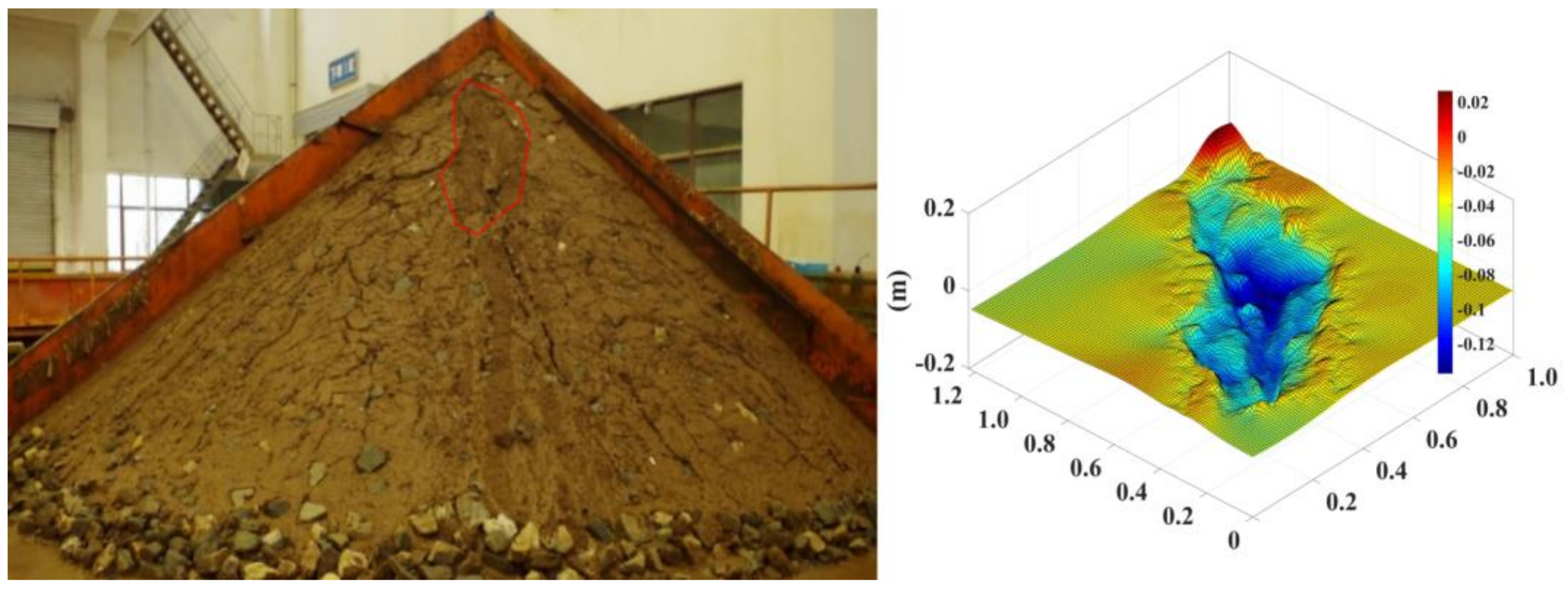
2.4. Surface Elevation Sampling

Before the first rainfall and after each rainfall, the slope surface was scanned using a Leica Nova MS50 device mounted on a tripod and positioned at 3–4 m vertically above the slope surface (Figure 1). The laser beam diameter was 8 mm × 20 mm at 50 m. The ranging accuracy was 2 mm + 2 ppm (high speed, without prism), and the vertical and horizontal resolution was up to 0.6 mm.
Five point-cloud data files were obtained in each complete experiment. Before the first scan, three points were marked to determine the position of the spoil heap slope in the set coordinate system. The three points were used as calibration points in subsequent scans, with the stipulation that the deviations of the three points must be no more than 3’’. This ensured that the obtained five point-cloud data files were in the same coordinate system, and the registration step was saved [27]. Each point-cloud data file contained ~240,000 elevation points covering a slope area of ~11.54 m2 at a 5-mm sample interval.

2.5. Drainage Network Delineation

Digital elevation models (DEMs) were generated utilizing the scanned points in ArcGIS (version 10.4, environmental systems research institute, Redlands, California, USA) software. The drainage network was delineated based on the DEMs using the steepest descent algorithm, D8 [28]. The procedure consists of three steps: (1) The pits (local depressions) are filled by increasing the elevation until they drain; (2) the flow direction is determined for each cell within the DEM: in the D8 algorithm, and the flow direction is assigned to the particular cell of the eight neighboring cells with the steepest descent; and (3) the number of cells that drain through each cell (contributing area) is determined by counting. From the resulting data set, streams are defined as those cells that have a contributing area above a certain threshold value. Finally, the raster drainage network is vectorized, and the streams are ordered by the Strahler method [17].

2.6. Drainage Network Characterization

2.6.1. Network Configuration

Drainage density and stream frequency describe the network configuration. The drainage density Ds (m/m²) is computed as:
D s = j = 1 n L j A
where n is the highest stream order; L(j) is the length of the streams of order j (j = 1···n) (m); j = 1 n L j is the sum of the flow lengths through all network (m); and A is the total drainage area (m²).
Stream frequency F (/m²) is calculated by
F = j = 1 n N j A
where N(j) is the number of the streams of order j (j = 1···n), so j = 1 n N j is the total number of the streams in the whole network.

2.6.2. Stream Characteristics

Sinuosity and gradient describe individual stream characteristics. For each drainage network, three streams were randomly selected on the left-hand, middle, and right-hand sides of the slope to calculate their sinuosity and gradient (a total of nine streams). The average values represent the sinuosity and gradient of this network.
For the individual stream, the sinuosity and gradient are determined as follows:
Sinuosity :   S = L m x 2 + n y 2
Gradient :   G % = 100 Z x y Z m n L
where L is the stream length (m); x and y, respectively, denote the horizontal and vertical coordinates of an endpoint of the stream (m); m and n, respectively, denote the horizontal and vertical coordinates of another endpoint of the stream (m); and Zxy and Zmn are the elevation of the two endpoints (m).

2.6.3. Fractal Dimension

Fractal dimension (D) describes the network organization. Multifractal characteristics of drainage networks were calculated by the box counting method [29], which takes a set of data and attempts to cover (enclose) the entire data set with a minimal number of adjacent, equal-sized boxes. In this study, to estimate D, the drainage network was covered multiple times using varying box sizes. In terms of box counting, D is given by
D = lim r 0 l o g N r l o g 1 / r
where N(r) is the number of boxes that contain at least one piece of the network; and r is the size of the box (r = 1, 2, 4, …, 16 cm).
A plot of log (N(r)) vs. log (1/r) should theoretically be a straight line with a slope equal to D [29].

2.7. Hydrodynamic Parameters of Runoff

The shear stress τ (N/m2) is defined as the drag force exerted by the flowing water on soil surface per unit bed area and is calculated as follows:
τ = γ m g R J
where γm is the mass density of the water/sediment mixture (kg/m3); g is the acceleration due to gravity ( g = 9.8 m/s2); J is the hydraulic gradient, which is approximately substituted by the sine of the slope gradient [30]; and R is the hydraulic radius, which is considered to be equal to the flow depth in overland flow conditions (m) [31]. The flow depth is difficult to measure because it is too shallow and because of the dynamic conditions [32]. Therefore, a simplification was made in which the flow depth was assumed to be uniform. Then, the mean flow depth h (m) was calculated using the procedure in Xiao et al. [31]:
h = R t v W
where Rt is the instant runoff (m3/s); v is the flow velocity (m/s); and W is the mean flow width (m). Runoff spread evenly on the flat slope surface at the beginning of experiment, and W in the first rainfall event (W1) was regarded as the average width of the three measure sections, 2.748 m. In subsequent rainfalls, the flow width was decreased because of the runoff convergence, and therefore, the mean flow width was calculated as:
W n = 2.748 × D s n D s 1
where Ds1 is the drainage density of the first rainfall; n (n = 2, 3, 4) is the sequence number of the rainfall event.
The unit energy of water-carrying section e (m) reflects the sum of the kinetic energy and potential energy of the flow at the base of the lowest water-carrying section, which is:
e = a · v 2 2 g + h
where a is a kinetic energy correction factor (a = 1).
The stream power   ω (N/(m·s)) represents the rate of expenditure of the potential energy of the runoff water on the soil surface per unit bed area, determined as:
ω = τ v

3. Results

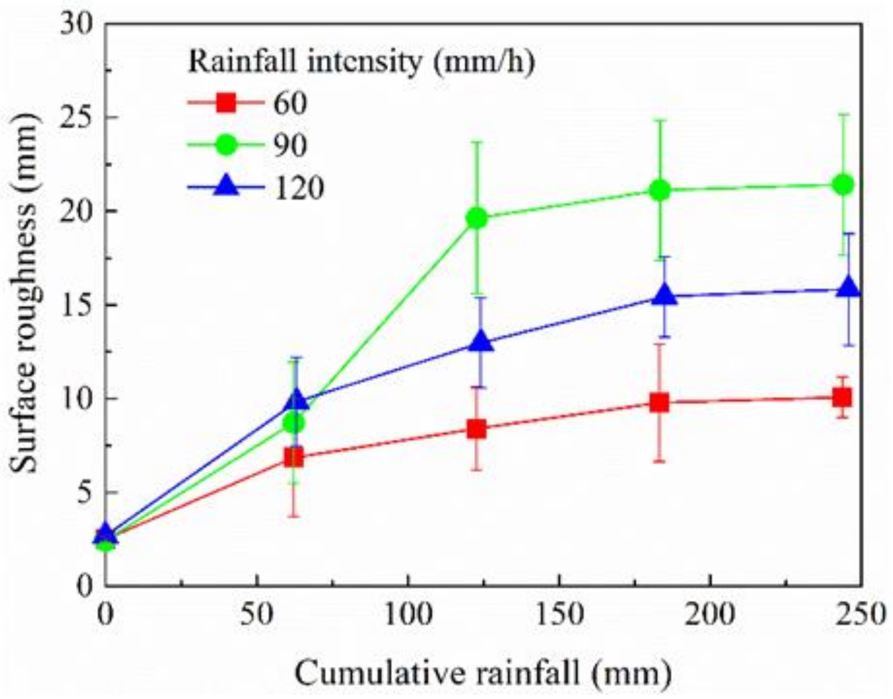
3.1. Soil Surface Roughness

Surface roughness characterizes the undulations in the micro-topography. As can be seen in Figure 2, for the three rainfall intensity treatments, roughness increased with cumulative rainfall and tended to stabilize after 120 mm precipitation. According to experimental observation, raindrops falling on the exposed rock fragments were gathered into runoff from the lower edge of the fragments, strengthening the erosion force sufficiently to develop small rills. At the same time, dispersed soil particles were moved downhill due to the steep slope. As a result, the initial smooth and level surface gradually became fragmented during the first two rainfall events due the rill and inter-rill erosion, and the roughness increased accordingly. After 120 mm of rainfall, the variability of the roughness decreased, indicating that the erosion pattern had stabilized, and the further development of rills became dominated.
Greater rain intensity resulted in increased roughness. The overall surface roughness for a rainfall intensity of 120 mm/h was about 1.5 times that following 60 mm/h intensity. However, 90 mm/h rainfall intensity sharply increased the roughness after 60 mm of rain had accumulated, and it was then much larger than for the other two treatments (Figure 2). This was due to a partial landslide on the upper slope during the second rainfall event (accumulated rainfall 60–120 mm) at 90 mm/h intensity (Figure 3). A concave slip-surface zone remained on the surface after the landslide, increasing the undulation degree and greatly increasing the roughness.

3.2. Relationship between the Total Stream Length and Critical Flow Accumulation Area

When extracting a drainage stream network from DEM data, it is necessary to identify a flow accumulation threshold because there is a certain correlation between the value of the threshold and the generated total stream length [16]. The flow accumulation threshold is a parameter of the D8 algorithm whose suitable determination allows sectioning of DEM cells that represent drainage networks. Stream networks are generated from DEMs, and the total stream length is calculated for a threshold range 0–250 cm2. The total length of streams decreases when the threshold becomes larger, with a strong exponential correlation (R2 > 0.9) (Figure 4). The optimal threshold is taken to be the corresponding value where the curve tends to be smooth. In this study, the threshold was 137.5 cm2 (dashed vertical line in Figure 4).

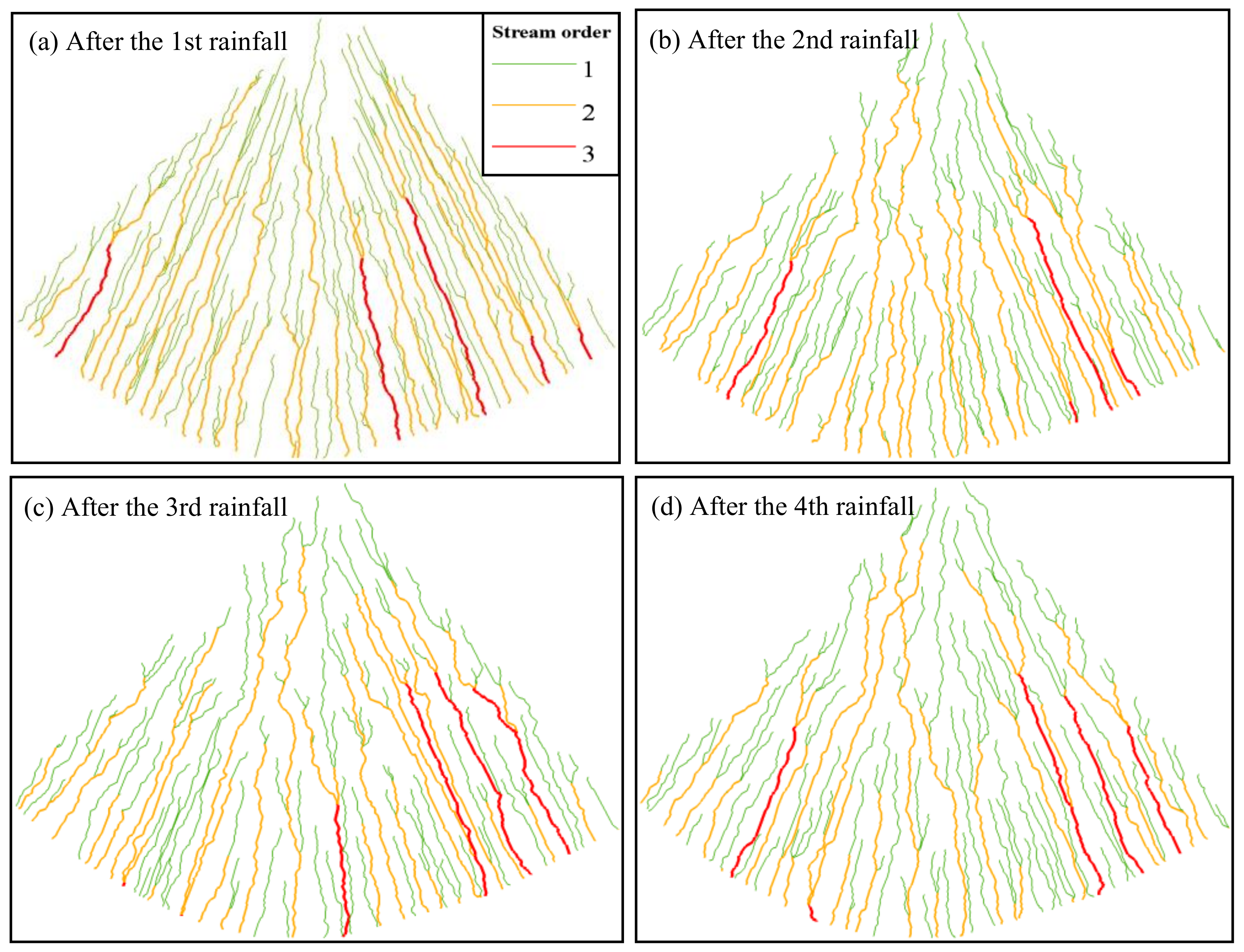
3.3. Characteristics of a Developing Drainage Network

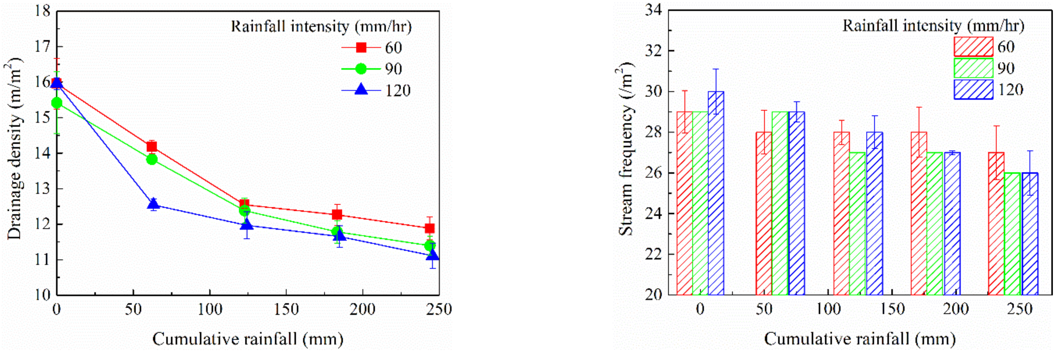
3.3.1. Drainage Density and Stream Frequency

Drainage density and stream frequency reflect the total length and the total number of flow paths per unit area, respectively.
Figure 5 shows that the drainage density decreased with cumulative rainfall, indicating the decreasing total length of flow paths. The initial drainage density, 15.42–15.96 m/m2, was reduced to 11.107–11.884 m/m2 after four rainfalls. A decrease of 21.3%, 19.7%, and 25.0% occurred in the first two rainfalls for the three rainfall intensity treatments, respectively. This indicated the stronger effect of the first accumulated 120 mm rainfall on the drainage network structure on the spoil heap slope.
The initial slope surface was nearly smooth; after the first rainfall, the soil surface developed a primary undulating shape as a primary erosive terrain, on which preferential flow paths (not yet well-developed rills) were observed (Figure 6a). Subsequently, flow paths gradually converged, and the network became sparser. After the second rainfall, the scope and structure of the networks was mostly developed (Figure 6b). In the next two rainfalls, rill incision continued to develop on the primary eroded terrain, which enhanced the degree of concentration of the drainage networks. As a result, the drainage density decreased with cumulative rainfall. Moreover, smaller rainfall intensity seemed to correspond to larger drainage density (Figure 5), but the overall difference between treatments was not significant (* p > 0.05).
The stream frequency was 26–30/m2, slightly decreasing with cumulative rainfall, and varying insignificantly between treatments (Figure 5). In general, little change was evident in stream frequency, but conversion of the path order was apparent. All networks showed a maximum order of three (STRAHLER classification method [17]).
As Figure 7 shows, the number of first-order streams decreased by 18, 21, and 24 with cumulative rainfall for the three rainfall intensity treatments, respectively. For the second-order stream, the path number first increased and then decreased with cumulative rainfall for the 60 and 90 mm/h rainfall intensity and gradually decreased at 120 mm/h rainfall intensity. This indicated that the greater rainfall intensity led to a more intense runoff convergence process. The number of third-order streams ranged between 2 and 7, which increased with rainfall sequence and did not differ obviously between rainfall intensity. The decreasing number of low-level streams and the increase of high-level streams reflected a process in which low-level runoffs merged into higher-level runoffs as a result of rill development and the runoff concentration. Therefore, the stream frequency decreased.

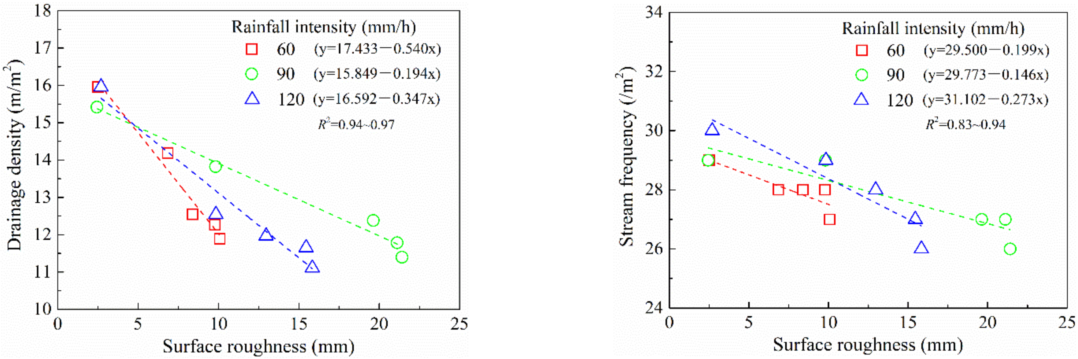
3.3.2. Relationship between Roughness and Drainage Density and Stream Frequency

In Figure 8, for the three rainfall intensity treatments, the surface roughness shows close negative correlations with drainage density (R2 = 0.94–0.97) and stream frequency (R2 = 0.67–0.83). On the rougher surface, coarser units (e.g., exposed rock fragments and rill incision) with sizes greater than the flow depth caused a higher degree of runoff convergence. Rougher surfaces roughness resulted in smaller areas of the surface contributing to runoff. Hence, drainage density and stream frequency decreased with increasing roughness. However, the degree of roughness had no obvious influence on the network structure for the different rainfall intensities.

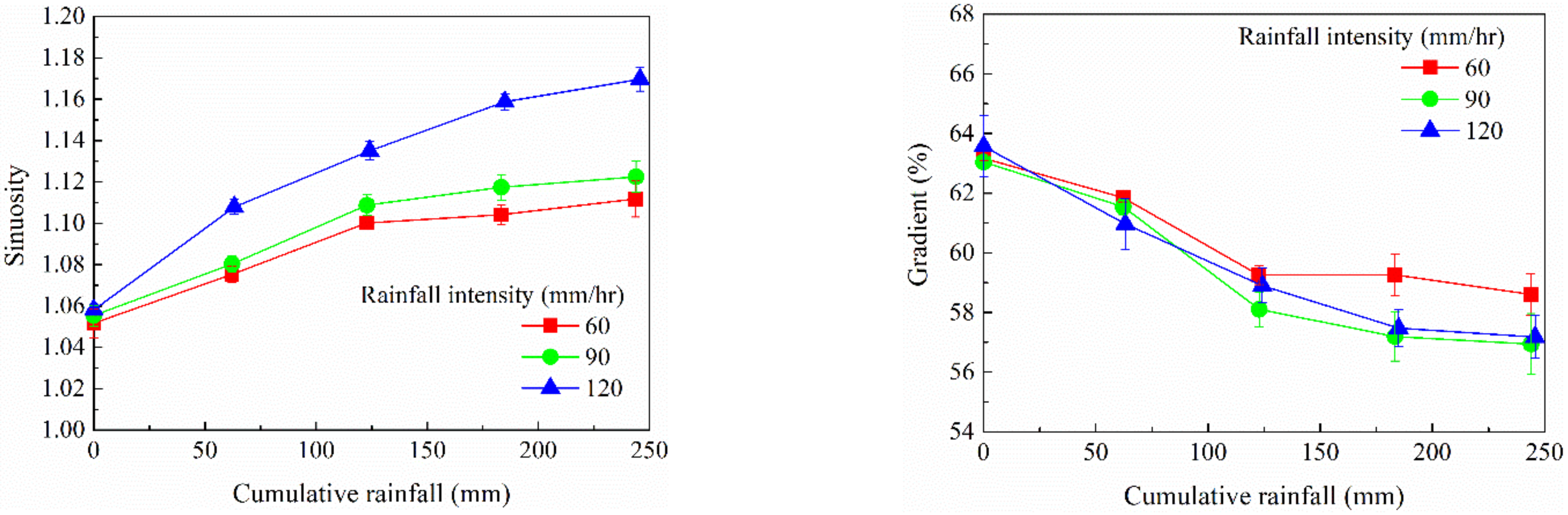
3.3.3. Flow Path Sinuosity and Gradient

Sinuosity and gradient are indicators that describe the shape of individual flow path. Sinuosity indicates the degree of meander of the flow path. As shown in Figure 9, the initial sinuosity was 1.052–1.058 and was not significantly different for the three rainfall intensities but increased with cumulative rainfall to a final value of 1.107–1.170 (* p < 0.05). It can be seen from Figure 6 that the increasing sinuosity with rainfall sequence corresponded to more flow path convergence, which indicates a longer individual path.
As the cumulative rainfall increased, higher orders of streams were collected from the lower orders in furrows to improve network organization (Figure 6). In this process, as the network became increasingly sparse, the flow paths became more meandering (i.e., the sinuosity increased). Between treatments, the sinuosity was ordered as 2.0 > 1.5 > 60 mm/h, which may relate to the change of surface roughness between rainfall intensity treatments. For 60 and 120 mm/h intensities, a larger surface roughness was related to a more broken surface, resulting in more sinuous flow paths; however, for 90 mm/h intensity, the maximum roughness caused by the landslide did not correspond to the maximum sinuosity. This is discussed further below.
The gradient indicates the rate of change of the flow path elevation change in the flow direction. Figure 9 shows that the initial gradient was 63.04–63.57%, being close to the natural slope of spoil heaps (64.94%), for all three treatments. After four rainfalls, the gradient flattened to 57.17–58.60%, with little difference between treatments.
A longer flow path length or a smaller difference in elevation between the ends of the flow path both equate to a flatter gradient. For a given rainfall intensity, extension of the actual flow path (i.e., increased sinuosity) contributed to a flatter gradient with rainfall sequence. For 60 and 120 mm/h rainfall intensity, the end-to-end elevation differences of flow paths were comparable, at 1.61–1.74 m and 1.62–1.70 m, respectively. Therefore, the lesser gradient observed for the 120 mm/h intensity rainfall event was mainly due to the greater sinuosity. For the 90 mm/h intensity, the gradient was least. In addition to the median sinuosity, this also coincided with the least end-to-end elevation difference of the flow path (1.37–1.70 m). For the 90 mm/h intensity treatment, the landslide on the upper slope caused a partial surface depression, resulting in reduced end-to-end elevation differences for flow paths at that location. The landslide, which occurred during the second rainfall event at 90 mm/h intensity, corresponded to the significant drop in the third gradient point in Figure 9.

3.3.4. Relationship between Roughness and Stream Sinuosity and Gradient

For the three rainfall intensity treatments, surface roughness was correlated well (positive) with stream sinuosity (R2 = 0.94–0.97) and was less clearly negatively correlated with stream gradient (R2 = 0.67–0.83) (Figure 10). Due to surface undulation, the runoff flowed only along lower places, resulting in longer and more sinuous flow paths. The increased sinuosity reduced the rate of change of elevation in the direction of the flow paths, which is to say that the gradient decreased.

3.4. Fractal Dimension of the Drainage Network

Fractal dimensions are a comprehensive indicator of network structure, density, and organization. Larger fractal dimensions imply a more intricate and intensive network. Table 1 shows that the fractal dimension varied in the range of 1.350–1.454, 1.305–1.459, and 1.292–1.455, respectively, for the three rainfall intensities. For a given rainfall intensity, the fractal dimension gradually decreased with rainfall sequence, indicating the convergence of the drainage network. This confirms the results of the decreasing drainage density and stream frequency with cumulative rainfall (Figure 5).
The average fractal dimension was 1.389, 1.355, and 1.338, respectively for the three rainfall intensities, but the difference was not statistically significant overall (* p > 0.05). However, after the first rainfall, the differences in fractal dimensions for the three treatments became obvious (* p < 0.05). The fractal dimension was reduced when the rainfall intensity increased, indicating that the drainage network tended to be concentrated and simplified. After the second rainfall (third-order scan), the difference between the fractal dimensions for the 1.5 and 120 mm/h intensity treatments was not significant. This is most possibly related to the landslide during the 90 mm/h rainfall. The depressed area on the upper slope caused by the slip surface of the landslide was conducive to the runoff collection during subsequent rainfall events, leading to fewer branches in the drainage network at that location. Consequently, the fractal dimension after the second rainfall for 90 mm/h intensity treatment was lowered and became close to the value for the 120 mm/h intensity treatment.

3.5. Relationship between Hydrodynamic Parameters and Drainage Network Characteristics

The runoff is the main factor affecting the hydrodynamics parameters. In this study, the total runoff coefficients (ratio of runoff to rainfall) were 0.686, 0.595, and 0.516 for 60, 90, and 120 mm/h rainfall intensities, respectively. The runoff rate for each rainfall event had a highly significant positive correlation with shear force, unit energy of the water-carrying section, and water flow power (r > 0.9) (Table 2). Therefore, when analyzing the correlation between the characteristic parameters of the flow network and the hydrodynamic parameters, the influence of runoff rate was eliminated using a partial correlation analysis.
The flow velocity was significantly correlated with all four drainage network parameters (Table 2), indicating the sensitive response of the flow velocity to the evolution of drainage network. The decreases of the drainage density and stream frequency mean that the runoff tended to be concentrated and the runoff flux increased; hence, the flow velocity increased accordingly. The gradient implies the gravitational potential energy of the water flow, which is positively related to the flow velocity. The larger stream sinuosity means the more winding path the flow took, to which the flow rate should seemingly have a negative response. However, the flow velocity also positively correlated with the stream sinuosity.
For the three hydrodynamic parameters, the shear stress was found to have no significant relationship with the four drainage network parameters. The unit energy of water-carrying section only had a significant positive correlation with the stream frequency. The stream power is the only one hydrodynamic parameter that was more sensitive to the change of drainage network, which is closely related to drainage density, stream sinuosity, and gradient (r = −0.644, 0.832, −0.719, respectively). It can be inferred that stream power is a superior parameter to describe the erosion and hydrological processes for spoil heap slopes.
Table 3 lists the fitting equations of the lines of best fit for stream power, runoff rate, and three drainage network parameters. It is seen that linear equations satisfactorily express the relationships between stream power and the three variables of drainage network characteristic (R2 = 0.961 to 0.979).

4. Discussion

The results of the present study show an increasing surface roughness with cumulated rainfall, which is in contrast to those for tilled surfaces [33,34]. Generally, tilled surfaces have larger initial roughness due to the artificial soil ridges or excavation [32]. As the cumulative rainfall increases, the soil at the bulge is eroded and transported to lower-lying places and deposited. Hence, the undulating soil surface gradually becomes gentle and less rough under the flattening effect of runoff [35,36]. The initial surface of a spoil heap, however, tends to be initially smooth after dumping, with a smaller roughness. Moreover, the steepness of the slope caused the eroded soil to be transported out of the slope rather than being deposited there [1], making the spoil heap surface increasingly uneven and developing rills [37]. As a result, the surface roughness gradually increases with cumulated rainfall. Under 90 mm/h rainfall, landslide occurred due to a weak layer in the material that was gradually infiltrated and softened by runoff water [38].
Observations showed visible cracks developing on the slope because the topmost soil shrank after being soaked in first rainfall. In the following rainfall, rainwater entered the cracks and infiltrated downhill inside the soil, creating conditions for the formation of weak layers [39]. The infiltration was least at 60 mm/h rainfall intensity, with a maximum runoff coefficient of 0.686, and few obvious cracks formed on the slope. At 120 mm/h rainfall intensity, more cracks were formed, but the rainfall duration (30 min) was too short for runoff to infiltrate and form the weak layer. Therefore, only at 90 mm/h intensity were both conditions met to trigger a landslide.
For any given rainfall intensity, increasing roughness negatively correlated with drainage density and stream frequency, leading to a more sinuous flow and a reduced flow path gradient. This is consistent with the results of the initial smooth slopes in Helming et al. [17] and Romkens et al. [40]. On a smooth soil bed, such as a spoil heap slope, the flow becomes concentrated into fewer flow paths, each causing a deeper incision during rainfall [20].
In the present case, the drainage network gradually became more convergent and organized in rainfall sequence on spoil heap slope, accompanied by the adjustment of the low-order streams towards higher-order streams. For other initial rough-surface types, such as agricultural hillslope or tilled soil surfaces, however, the effects are often reversed; that is, as rainfall cumulates, drainage density increases, and flow path sinuosity decreases due to the flattening effect of runoff in those contexts [13,40].
Our results show that drainage density, runoff frequency. and fractal dimension did not differ greatly for the different rain intensities. The landslide that occurred during 90 mm/h rainfall caused the greatest roughness of the slope surface but had little effect on the drainage network structure. The reason may be that, first, regardless of whether a landslide occurred, the erosion processes were the same with rainfall as the driving force. The inherent runoff generation and routing pattern that formed flow paths (including rills) along the slope resulted in similar drainage network structures for all three rainfall intensity treatments. Second, since the landslide occupied a small area on the upper slope, the influence of increased roughness caused by landslides on the whole drainage network is not reflected. Rather, its influence lies in expanding the collection area of several flow paths and in the deeper incision of the paths (including rills) [41].
Moreover, the difference in surface roughness caused by the 60–120 mm/h rainfall intensity treatments in our study was 2.9–11.3 mm, which was smaller than the contrast in the initial roughness reported for other studies [20,21]. Hence, it did not lead to obvious differences in drainage pattern and intensity, which explains why the drainage density did not vary significantly between different rainfall intensities.
The fractal dimensions of drainage networks were in the range of 1.305–1.455, which is larger than for some tillage landforms with gentler slope [20,42], indicating a more highly developed and more highly organized drainage network on spoil heap slopes. In addition, although the fractal dimension showed a gentle increase with increasing rainfall intensity, consistent with Luo et al. [20], the small differences in the results for the various rain treatments also suggests that, for spoil heaps, the mechanisms controlling the evolution of drainage networks were affected by the rainfall intensities to a relatively minor extent.
The relationship between drainage network development and the dynamic erosive process of the soil surface relies on concentration of the flow into the fewer drainage paths [17]. Among the hydrodynamic parameters, the stream power most closely reflected the drainage network evolution, which became greater with runoff concentration, indicated by the significant correlations between stream power and drainage density and between stream sinuosity and gradient. The sinuosity positively related to the stream power, with largest correlation coefficient. This result is similar to what was reported by Helming et al. [17], in which the sinuosity was 1.2–1.4 on a tillage slope, a larger range than the 1.052–1.170 for a spoil heap slope. Therefore, the flow paths on the spoil heap were not meandering enough to extend the total flow path and increase the energy consumption of runoff flowing, and thus reduce the flow velocity and its stream power. In addition, the steep gradient (57.17–63.57%, much steeper than a tilled field) is another reason that the sinuosity did not play a negative role [17,42]. Instead, the erosive terrain development on a spoil heap slope gradually changing from flat to a complex terrain of rills led to an increase in flow velocity [42]. Hence, the increase in sinuosity accompanied by flow path convergence enhanced the hydrodynamic forces acting on the runoff.

5. Conclusions

Drainage network features and surface roughness on spoil heaps were investigated by simulating successive rainfall at different intensities. Surface roughness increased with cumulative rainfall at each rainfall intensity and had significant negative correlations with both drainage density and stream frequency. Correspondingly, flow paths gradually tended to converge during rainfall, leading to increased sinuosity and a decreasing gradient of individual streams.
Generally, the greater rainfall intensity roughness resulted in a larger surface roughness on the spoil heaps, but during the 90 mm/h intensity rain event (the median value in this study), a landslide occurred on the upper slope of the spoil heap, resulting in the largest roughness. The difference in roughness for the different simulated rainfall intensities did not cause distinctly different drainage network features. Comparable fractal dimension also indicated that the effect of different rainfall intensity on drainage network structure was not significant.
Of the hydrodynamic parameters, stream power was found to be more closely related to the characteristic parameters of the drainage network than others. The relationships between stream power and the three characteristic variables of drainage network were expressed by linear equations with R2 values between 0.961 and 0.979.

Author Contributions

Conceptualization, Y.X. and H.L.; methodology, J.L.; software, D.C.; validation, D.C., J.L., H.L. and Y.X.; formal analysis, D.C.; investigation, D.C. and J.L.; resources, H.L.; data curation, D.C. and J.L.; writing—original draft preparation, D.C.; writing—review and editing, J.L.; visualization, D.C. and J.L.; supervision, H.L.; project administration, H.L.; funding acquisition, H.L. All authors have read and agreed to the published version of the manuscript.

Funding

This research was funded by the Natural Science Foundation of China, grant number 41601300.

Institutional Review Board Statement

Not applicable.

Informed Consent Statement

Not applicable.

Data Availability Statement

Not applicable.

Acknowledgments

This work was supported by the Natural Science Foundation of China (41601300).

Conflicts of Interest

The authors declare no conflict of interest.

References

  1. Luo, H.; Rong, Y.; Lv, J.; Xie, Y. Runoff erosion processes on artificially constructed conically-shaped overburdened stockpiles with different gravel contents: Laboratory experiments with simulated rainfall. Catena 2019, 175, 93–100. [Google Scholar] [CrossRef]
  2. Cerda, A. Soil water erosion on road embankments in eastern Spain. Sci. Total Environ. 2007, 378, 151–155. [Google Scholar] [CrossRef] [PubMed]
  3. Rodrigues, S.C.; Silva, T.I. Dam Construction and Loss of Geodiversity in the Araguari River Basin, Brazil. Land Degrad. Dev. 2012, 23, 419–426. [Google Scholar] [CrossRef]
  4. Zhao, X.; Xie, Y.S.; Jing, M.X.; Yang, Y.L.; Li, W.H. Standardization parameter for spoilbank underlying surface simulation of development construction project. J. Soil Water Conserv. 2012, 26, 229–234. [Google Scholar]
  5. Wang, G.; Innes, J.; Yusheng, Y.; Shanmu, C.; Krzyzanowski, J.; Jingsheng, X.; Wenlian, L. Extent of soil erosion and surface runoff associated with large-scale infrastructure development in Fujian Province, China. Catena 2012, 89, 22–30. [Google Scholar] [CrossRef]
  6. Peng, X.; Shi, D.; Jiang, D.; Wang, S.; Li, Y. Runoff erosion process on different underlying surfaces from disturbed soils in the Three Gorges Reservoir Area, China. Catena 2014, 123, 215–224. [Google Scholar] [CrossRef]
  7. Reddy, K.R.; Basha, B.M. Slope Stability of Waste Dumps and Landfills: State-of-the-Art and Future Challenges. In Proceedings of the Indian Geotechnical Conference, Kakinada, India, 18–20 December 2014. [Google Scholar]
  8. Jimenez, M.D.; Ruiz-Capillas, P.; Mola, I.; Pérez-Corona, E.; Casado, M.A.; Balaguer, L. Soil Development at the Roadside: A Case Study of a Novel Ecosystem. Land Degrad. Dev. 2013, 24, 564–574. [Google Scholar] [CrossRef]
  9. Nearing, M.A.; Xie, Y.; Liu, B.; Ye, Y. Natural and anthropogenic rates of soil erosion. Int. Soil Water Conserv. Res. 2017, 5, 77–84. [Google Scholar] [CrossRef]
  10. Shi, D.; Wang, W.; Jiang, G.; Peng, X.; Yu, Y.; Li, Y.; Ding, W. Effects of disturbed landforms on the soil water retention function during urbanization process in the Three Gorges Reservoir Region, China. Catena 2016, 144, 84–93. [Google Scholar] [CrossRef]
  11. Nearing, M.A.; Foster, G.R.; Lane, L.J.; Finkner, S.C. A Process-Based Soil Erosion Model for USDAWater Erosion Prediction Project Technology. Am. Soc. Agric. Eng. 1989, 32, 1587–1593. [Google Scholar] [CrossRef]
  12. Morgan, R.P.; Quinton, J.N.; Smith, R.E.; Govers, G.; Poesen, J.W.; Auerswald, K.; Chisci, G.; Torri, D.; Styczen, M.E. The European Soil Erosion Model (EUROSEM): A dynamic approach for predicting sediment transport from fields and small catchments. Earth Surf. Process. Landf. 1998, 23, 527–544. [Google Scholar] [CrossRef]
  13. Peñuela, A.; Darboux, F.; Javaux, M.; Bielders, C.L. Evolution of overland flow connectivity in bare agricultural plots. Earth Surf. Process. Landf. 2016, 41, 1595–1613. [Google Scholar] [CrossRef] [Green Version]
  14. Guo, M.; Shi, H.; Zhao, J.; Liu, P.; Welbourne, D.; Lin, Q. Digital close range photogrammetry for the study of rill development at flume scale. Catena 2016, 143, 265–274. [Google Scholar] [CrossRef]
  15. Zhang, X.; Zhou, Y.; Dong, Y.; Zhang, H.; Zhang, C.; Zhang, Q. Measurement of the connectivity of runoff source areas on a bare soil surface in a laboratory experiment. J. Soil Water Conserv. 2019, 74, 513–519. [Google Scholar] [CrossRef]
  16. Martz, L.W.; Garbrecht, J. Automated extraction of drainage network and watershed from digital elevation models. J. Am. Water Resour. Assoc. 1993, 29, 901–908. [Google Scholar] [CrossRef]
  17. Helming, K.; Römkens, M.J.; Prasad, S.N.; Sommer, H. Erosional development of small scale drainage networks. Process. Model. Landf. Evol. 1999, 78, 123–145. [Google Scholar]
  18. Horton, R. Erosional development of streams and their drainage basins: Hydrological approach to quantitative morphology. GSA Bull. 1945, 56, 275–370. [Google Scholar] [CrossRef] [Green Version]
  19. Carvajal, F.; Aguilar, M.A.; Agüera, F.; Aguilar, F.J.; Giraldez, J.V. Maximum Depression Storage and Surface Drainage Network in Uneven Agricultural Landforms. Biosyst. Eng. 2006, 95, 281–293. [Google Scholar] [CrossRef]
  20. Luo, J.; Zheng, Z.; Li, T.; He, S. Spatial heterogeneity of microtopography and its influence on the flow convergence of slopes under different rainfall patterns. J. Hydrol. 2017, 545, 88–99. [Google Scholar] [CrossRef]
  21. Gómez, J.A.; Darboux, F.; Nearing, M.A. Development and evolution of rill networks under simulated rainfall. Water Resour. Res. 2003, 39, 93–94. [Google Scholar] [CrossRef] [Green Version]
  22. Lv, J.; Luo, H.; Xie, Y. Impact of rock fragment size on erosion process and micro-topography evolution of cone-shaped spoil heaps. Geomorphology 2020, 350, 106936. [Google Scholar] [CrossRef]
  23. Bennett, S.J.; Gordon, L.M.; Neroni, V.; Wells, R.R. Emergence, persistence, and organization of rill networks on a soil-mantled experimental landscape. Nat. Hazards 2015, 79, S7–S24. [Google Scholar] [CrossRef]
  24. IUSS Working Group WRB. World Reference Base for Soil Resources 2014, Update 2015 International Soil Classification System for Naming Soils and Creating Legends for Soil Maps. In World Soil Resources Reports No. 106; FAO: Rome, Italy, 2015. [Google Scholar]
  25. Zheng, F.; Zhao, J. A brief introduction on the rainfall simulation laboratory and equipment. Res. Soil Water Conserv. 2004, 11, 177–178. (In Chinese) [Google Scholar]
  26. Zhang, P.; Yao, W.; Tang, H.; Wei, G.; Wang, L. Laboratory investigations of rill dynamics on soils of the Loess Plateau of China. Geomorphology 2017, 293, 201–210. [Google Scholar] [CrossRef]
  27. Wheaton, J.M.; Brasington, J.; Darby, S.E.; Sear, D.A. Accounting for uncertainty in DEMs from repeat topographic surveys: Improved sediment budgets. Earth Surf. Process. Landf. 2010, 35, 136–156. [Google Scholar] [CrossRef]
  28. O’Callaghan, J.F.; Mark, D.M. The extraction of drainage networks from digital elevation data. Comput. Vis. Graph. Image Process. 1984, 27, 323–344. [Google Scholar] [CrossRef]
  29. Jaya, V.; Raghukanth, S.T.G.; Mohan, S.S. Estimating fractal dimension of lineaments using box counting method for the Indian landmass. Geocarto Int. 2014, 29, 314–331. [Google Scholar] [CrossRef]
  30. Zhang, L.T.; Gao, Z.L.; Yang, S.W.; Li, Y.H.; Tian, H.W. Dynamic processes of soil erosion by runoff on engineered landforms derived from expressway construction: A case study of typical steep spoil heap. Catena 2015, 128, 108–121. [Google Scholar] [CrossRef]
  31. Xiao, H.; Liu, G.; Liu, P.; Zheng, F.; Zhang, J.; Hu, F. Response of soil detachment rate to the hydraulic parameters of concentrated flow on steep loessial slopes on the Loess Plateau of China. Hydrol. Process. 2017, 31, 2613–2621. [Google Scholar] [CrossRef]
  32. Guo, T.; Wang, Q.; Li, D.; Wu, L. Sediment and solute transport on soil slope under simultaneous influence of rainfall impact and scouring flow. Hydrol. Process. 2010, 24, 1446–1454. [Google Scholar] [CrossRef]
  33. Xingming, Z.; Tao, J.; Xiaofeng, L.; Yanling, D.; Kai, Z. The temporal variation of farmland soil surface roughness with various initial surface states under natural rainfall conditions. Soil Tillage Res. 2017, 170, 147–156. [Google Scholar] [CrossRef]
  34. Bauer, T.; Strauss, P.; Grims, M.; Kamptner, E.; Mansberger, R.; Spiegel, H. Long-term agricultural management effects on surface roughness and consolidation of soils. Soil Tillage Res. 2015, 151, 28–38. [Google Scholar] [CrossRef]
  35. Zhao, L.; Wang, L.; Liang, X.; Wang, J.; Wu, F. Soil surface roughness effects on infiltration process of a cultivated slopes on the Loess Plateau of China. Water Resour. Manag. 2013, 27, 4759–4771. [Google Scholar] [CrossRef]
  36. Zhao, L.; Huang, C.; Wu, F. Effect of microrelief on water erosion and their changes during rainfall. Earth Surf. Process. Landf. 2016, 41, 579–586. [Google Scholar] [CrossRef]
  37. Rong, Y.; Luo, H.; Xie, Y.; Wang, A. Effect of rainfall intensity on erosion and rill evolution of engineering piles. J. Sediment Res. 2016, 6, 12–18. [Google Scholar]
  38. Mukhlisin, M.; Naam, S.I. Effect of rock fragments on pore water pressure and slope stability at a hillslope. J. Geol. Soc. India 2015, 86, 337–343. [Google Scholar] [CrossRef]
  39. Hung, K.C.; Kosugi, K.I.; Lee, T.H.; Misuyama, T. The effects of rock fragments on hydrologic and hydraulic responses along a slope. Hydrol. Process. 2007, 21, 1354–1362. [Google Scholar] [CrossRef]
  40. Romkens, M.J.M.; Helming, K.; Prasad, S.N. Soil erosion under different rainfall intensities, surface roughness, and soil water regimes. Catena 2001, 46, 103–123. [Google Scholar] [CrossRef]
  41. Lima, J.D.; Abrantes, J. Can infrared thermography be used to estimate soil surface microrelief and rill morphology? Catena 2014, 113, 314–322. [Google Scholar] [CrossRef]
  42. Zhang, P.; Tang, H.; Yao, W.; Zhang, N.; Xizhi, L. Experimental investigation of morphological characteristics of rill evolution on loess slope. Catena 2016, 137, 536–544. [Google Scholar] [CrossRef]
Figure 1. Experimental equipment.
Water 13 03475 g001
Figure 2. Change of the soil surface roughness with cumulative rainfall (four rainfall sequence in four days, 60 mm/day, the same below).
Water 13 03475 g002
Figure 3. Photograph of spoil heap after the second rainfall at 90 mm/h intensity and the DEM of the landslide profile.
Water 13 03475 g003
Figure 4. Relationship between critical accumulation areas (threshold) and total stream lengths.
Water 13 03475 g004
Figure 5. Changes of drainage density and stream frequency with cumulative rainfall.
Water 13 03475 g005
Figure 6. Drainage networks evolution for the 90 mm/h rainfall intensity treatment (the stream order was classified by STRAHLER method), (ad) respectively shows the drainage network after the first to fourth rainfall.
Water 13 03475 g006
Figure 7. Changes of the steam numbers of different orders with cumulative rainfall (the stream order was classified by STRAHLER method).
Water 13 03475 g007
Figure 8. Relationships between surface roughness and drainage networks, stream frequency.
Water 13 03475 g008
Figure 9. Changes of the stream sinuosity and gradient of the stream paths with cumulative rainfall.
Water 13 03475 g009
Figure 10. Relationships between surface roughness, stream sinuosity, and stream gradient.
Water 13 03475 g010
Table 1. Fractal dimensions of networks on the surface after each rainfall event (LSD (least significant difference) test was conducted between three rainfall intensity treatments).
Scan Order
Rainfall Intensity (mm/h)12345
601.454a1.400b1.375b1.364b1.350b
901.459a1.387b1.315a1.309a1.305a
1201.455a1.333a1.305a1.304a1.292a
Table 2. Correlations between characteristic parameters of the drainage network (median values of the drainage density (Ds), stream frequency (F), stream sinuosity (S), and stream gradient (G)) and hydrodynamic parameters (mean flow velocity (v), shear stress (τ), unit energy of water-carrying section (e), and stream power (ω)).
Ds (m/m2)F (/m2)SG (%)Average Runoff Rate (mm/min)
v (m/s)−0.851 **1−0.881 **0.704 *0.940 **0.483 ns
τ (N/m2)0.480 ns−0.062 ns0.589 ns−0.461 ns0.960 **
e (m)−0.388 ns−0.683 *0.509 ns−0.482 ns0.934 **
ω (N/(m·s))−0.644 *−0.453 ns0.832 **−0.719 *0.932 **
1 ns, not significant; *: p < 0.05; **: p < 0.01.
Table 3. Fitting equations for stream power (ω), runoff rate (R), and three drainage network parameters (median values of the drainage density (Ds), stream sinuosity (S), stream gradient (G)).
Regression EquationR-SquareF-ValueSig.n
a 1bcEquation
ω = 0.503R − 0.019Ds + 0.2040.961111.0200.0320.0000.1500.00012
ω = 0.306R + 1.703S − 1.7940.979214.5390.0010.0020.0010.00012
ω = 0.537R − 0.011G + 0.5900.968135.3240.0000.0130.0300.00012
1 a, regression coefficient of R; b, regression coefficient of Ds, S, G; c is the constant term.
Publisher’s Note: MDPI stays neutral with regard to jurisdictional claims in published maps and institutional affiliations.

