
Using a Self-Organizing Map to Explore Local Weather Features for Smart Urban Agriculture in Northern Taiwan


Department of Bioenvironmental Systems Engineering, National Taiwan University, Taipei 10617, Taiwan
*
Author to whom correspondence should be addressed.
Water 2021, 13(23), 3457; https://doi.org/10.3390/w13233457
Submission received: 2 November 2021
/
Revised: 2 December 2021
/
Accepted: 2 December 2021
/
Published: 6 December 2021
(This article belongs to the Special Issue Artificial Intelligence Techniques in Hydrology and Water Resources Management)
Abstract
:Weather plays a critical role in outdoor agricultural production; therefore, climate information can help farmers to arrange planting and production schedules, especially for urban agriculture (UA), providing fresh vegetables to partially fulfill city residents’ dietary needs. General weather information in the form of timely forecasts is insufficient to anticipate potential occurrences of weather types and features during the designated time windows for precise cultivation planning. In this research, we intended to use a self-organizing map (SOM), which is a clustering technique with powerful feature extraction ability to reveal hidden patterns of datasets, to explore the represented spatiotemporal weather features of Taipei city based on the observed data of six key weather factors that were collected at five weather stations in northern Taiwan during 2014 and 2018. The weather types and features of duration and distribution for Taipei on a 10-day basis were specifically examined, indicating that weather types #2, #4, and #7 featured to manifest the dominant seasonal patterns in a year. The results can serve as practical references to anticipate upcoming weather types/features within designated time frames, arrange potential/further measures of cultivation tasks and/or adjustments in response, and use water/energy resources efficiently for the sustainable production of smart urban agriculture.
1. Introduction
Urban agriculture (UA), which is defined by the Food and Agriculture Organization (FAO) as “the small areas within the city for growing crops and raising small livestock or milk cows for own-consumption subsistence or small-scale sale in local/neighborhood markets” [1,2], takes advantage of vacant rooftops, balconies, and community spaces to plant vegetables for neighborhoods’ fresh diet in urban areas. In East Asia, Europe, and North America, many urban farmers produce potential high-quality food at an affordable cost [3]. Compared with large-scale commercial cultivation on rural farms, UA usually occupies smaller land areas and is operated by community volunteers/seniors (non-professionals) for leisure, social interaction, and partial self-sufficiency purposes [4,5]. Leafy vegetables are often the primary products of UA since they are highly valued for their nutritional content, with dietary diversity with shorter growing periods [6,7]. Therefore, the planting activities of UA generally produce short-term vegetable crops with more diversified species but less yield quantity and crop rotation is often carried out after each harvest upon the growers’ interests.
Weather plays a critical role in outdoor agricultural production by affecting the optimal growth, development, and yields of crops, as well as the incidence and spread of pests/diseases, water needs, and fertilizer requirements for cultivation. The spatiotemporal (short-term and annual) variations of weather factors (i.e., temperature, rainfall, humidity, sunshine, etc.) of a particular place over the selected time interval during the cultivation season should be considered for assessing their influences on crop growth. In addition, climate change has also caused impacts on agricultural operation and management [8,9].
Decision making in agriculture is based on knowledge of the crop behavior and cultivation information, which may also include characterization of the local growing conditions, management practices, and the response of the crop to these variables at any given time. In particular, the timing of planting, cultivation, and harvest based on cultural tasks are often determined based upon weather forecasts; therefore, a good climate-based strategy for agronomic planning can help to reduce the stresses of crop growth and increase the effectiveness of the timing of preventive measures and cultural operations, as well as engage farmers to organize and use appropriate cultural practices to cope with or take advantage of weather forecasts in various ways. On the other hand, once the crop season starts and resources demands and technology are committed, only certain cultivation operations can be adopted in response to weather phenomena by relying on advanced notice of the occurrence of erratic weather for minimizing the hazardous effects during mid-season [10].
Despite the agricultural weather forecast being available for upcoming days, many farmers in East Asia today still follow the traditional solar terms of the Lunar Calendar (also known as the Farmer Calendar or the Yellow Calendar in Chinese) from rural proverbs as important rules of thumb for the timing of cultivation practices in light of anticipating local weather in each season. Based on the experiences of ancestors, farmers are suggested to use specific agricultural operations for better efficiency due to the expectation for the occurrence of certain seasonal weather phenomenon on specific dates in a year.
In addition to nowcasting, short-term forecasts or monthly climate projections for agricultural producers are usually preferred by farmers when making agricultural decisions. The use of non-forecast climate information on seasonal pattern analysis, i.e., historical climate information, long-term climate outlooks, and decision calendars, can also be valuable as a practically useful reference for cultivation tasks and agricultural risk management [11,12]. The seasonal pattern of weather types requires probing into years of historical data of various weather factors, and feature patterns can be extracted through effective and efficient data-mining techniques to explore more information that might not otherwise be disclosed. Various machine learning methods were employed in precedent studies to classify weather features and make forecasts [13,14], for example, a deep neural network (DNN) for weather forecasting [15]; a recurrent neural network (RNN) and long short-term memory (LSTM) for air temperature forecasting [16]; an RNN for hourly rainfall forecasting during typhoon periods [17]; a multilayer perceptron neural network (MLP) for air temperature prediction inside greenhouse [18]; a convolutional neural network (CNN) for wind speed prediction [19] and weather pattern clustering [20]; a deep convolutional neural network (DCNN) for weather phenomenon classification based on images [21]; a backpropagation neural network (BPNN) for weather system prediction [22,23,24]; a self-organizing map (SOM) for estimating meteorological variables of evaporation [25], a method to train an SOM for clustering high-dimensional flood inundation maps [26]; an adaptive model of the enhanced multiple linear regression model (EMLRM) for rainfall forecasting [27]; a combined modular models comparison using moving average (MA), MLP, and support vector regression (SVR) for daily and monthly prediction on rainfall time series [28]; an artificial neural network (ANN)-based lower upper bound estimation (LUBE) and multi-objective fully informed particle swarm (MOFIPS) for interval forecasting for streamflow discharge [29]; and a comparison of BPNN, group method of data handing (GMDH), and autoregressive integrated moving average (ARIMA) for monthly rainfall forecasting [30].
As one of the powerful methods of exploratory data analysis for data mining and visualization interpreting [31,32], SOMs have been usually used to discover intrinsic patterns by downscaling the complex weather data sets from a high-dimensional space to a low-dimensional one through clustering similar data patterns into neighboring SOM units for easy comprehension [33,34]. For the feature extraction from large datasets, dimensionality reduction is a critical step to eliminate redundant information for simplifying the subsequent processes of classification and the search for information while retaining meaningful properties of the original datasets. Compared with traditional methods, such as principal component analysis (PCA) and wavelet decomposition methods, SOM may better classify datasets and present results in a two-dimensional topology well [35].
An increasing number of SOM applications were also adopted to assist with agricultural decision making when considering the weather information from recent years [36]. For agricultural applications, some data-driven models were developed to identify land covers for agricultural control and management and provide information for production systems to better manage their crops according to the specific conditions on farms [37,38,39,40]. Time series of climatic and agro-climatic indices were used to examine the signs of climate changes in rainfall, temperature, and agricultural drought to identify potential impacts on the agricultural water balance [41]. In addition, SOM was also applied to data clustering and pattern recognition for many types of climatic and meteorological data to analyze synoptic climatology at various spatial and temporal scales [42,43,44], forecasting and nowcasting [45,46,47], and investigation of extreme climate events [48,49,50], as well as variations of meteorological variables, such as evaporation and rainfall pattern analysis [25,51,52], cloud classification [53], and climate change analysis [54,55].
Generally, monthly/annual meteorological statistics provide very rough information about respective weather factors rather than substantially reflect the overall phenomenon of weather features during a certain period and give no characteristics on the temporal and sequential distribution of repetition and alteration trends. Weather forecasts are provided based on the surrounding atmospheric circulation condition. Both types of information are often used as reference guidelines for crop cultivation for farmers, but it is challenging for farmers to anticipate and grasp precisely what weather phenomena and features would potentially occur during a specific time window. Therefore, this research aimed to use data-mining techniques to discover/induce the annual pattern and distribution of weather types and features of a region based on historical meteorological data, including their occurrence time, frequency, continuity, and intensity, so that agricultural operationists can anticipate the occurrences and trends of weather types and features during each specified period for engaging in appropriate cultivation tasks in advance.
In this regard, this research adopted an SOM to cluster large and complex historical meteorological data into several categories (types) of similar weather features while exploring each type’s characteristics on temporal distribution, sequential continuity, occurrence time, and frequency so that crops can adapt to the weather in northern urban Taiwan owing to the measures that were taken beforehand (when necessary). Therefore, the eventual findings are expected to provide practical weather reference to help with sustainable production in terms of species selection, planting schedules, precautions arrangement, and further efficiency enhancement of water and energy resources that are used for the planning and design of urban agriculture/farming for promotion purposes.
2. Materials and Methodology
Various weather factors for agricultural forecasting are intertwined and affect farm planning and operations from place to place and from season to season. This research aimed to explore the representative spatiotemporal weather features by collecting and analyzing the observed data of 6 key weather factors at 5 weather stations in northern Taiwan. An SOM, as one of the effective artificial neural network approaches, was adopted to cluster the meteorological data to reveal the hidden weather features. Subsequently, the temporal patterns of such features at the Taipei Station were specifically examined so that potential measures in response to certain weather phenomena at certain periods for the smart and efficient utilization of resources (water/energy) in urban agriculture can be provided.
To cross-reference to the results of weather types and features, the Da-an rooftop farm, which has been a successful urban agriculture (UA) site since 2014 and had a complete work log and harvest records in Taipei City in northern Taiwan, was chosen as the real case in operation for reference. In addition, due to the special characteristics of UA, i.e., it usually involves smaller planting areas, lower harvest weight, higher crop rotation frequency, more species diversity, and short-term crops (with growing periods of a few months), the data collected during 2014–2018 were selected to form the weather types and features in this study.
2.1. Materials of Weather Data Collection
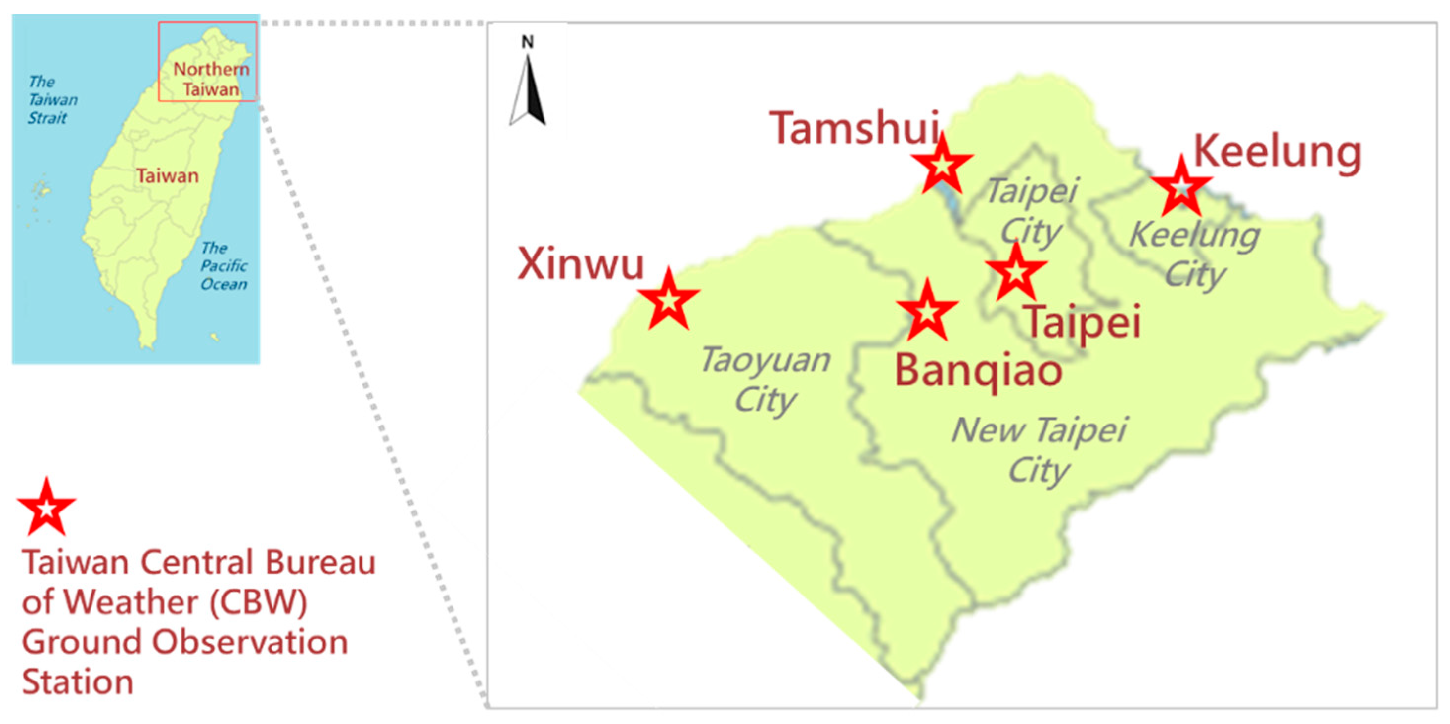
Taipei City, New Taipei City, Taoyuan City, and Keelung City, which constitute the main metropolitan area in northern Taiwan, were selected for this research. The four cities cover an area of 3675 km2 (accounting for 10.2% of the total area of Taiwan) and have a population of 8.82 million (about 38.3% of the total population of Taiwan). The daily meteorological data were collected from five Central Bureau of Weather (CBW) ground weather stations in northern Taiwan, including the Banqiao, Tamshui, Taipei, Keelung, and Xinwu Weather Stations (locations are shown in Figure 1) from 1 January 2014 to 31 December 2018 [56]. Being located in downtown areas in Taipei Metropolitan, the five weather stations were selected because they are governed directly by the Central Weather Bureau in Taiwan and can provide the most comprehensive, complete, and extensive monitoring weather data at urban areas in northern Taiwan. With Taipei City being located in the Taipei Basin and the Taipei Weather Station being situated in the main urban area in the city, the Taipei Weather Station was specifically examined to explore the weather types and features in this research because the Da-an rooftop farms, with its harvest logs for reference, was located there. With a similar approach, the weather types and patterns at the other four weather stations are also valuable and deserve further in-depth exploration in future research.
The meteorological factors (variables) for agricultural weather forecasts that immediately affect farm planning or operations vary from place to place and from season to season. According to the Köppen climate classification, Taiwan is an island that is classified as having a “warm oceanic climate/humid subtropical climate,” while Taipei City is classified as “temperate, no dry season, hot summer” (Köppen: Cfa) [57]. Temperature (for heat succession), relative humidity (for transpiration), precipitation (for irrigation), sunshine hours (insolation duration), global radiation (light and thermal condition for plant physiology), and total cloud cover (character of prevailing clouds that reduce the global solar radiation) are the core weather factors that influence crop-growing processes; therefore, each dataset comprised the daily logs of the 6 weather factors. Wind speed and direction were excluded from this research because the wind blowing around UA sites with a relatively small scale is often affected by the surrounding buildings. It is noted that these heterogeneous datasets were normalized (within a value range of 0–1.0) for preprocessing. Then, the normalized datasets were input into the SOM for clustering the weather features, and the clustering results were displayed in a honeycomb arrangement.
A total of 9130 datasets were collected from the 5 weather stations in northern Taiwan over the 5 years, and their basic statistics are given in Table 1.
2.2. Self-Organizing Map (SOM)
The SOM proposed by Kohonen in 1982 [58,59] is an artificial neural network that is configured with an unsupervised learning algorithm. It consists of repeatedly learning processes to gradually update the data nodes in the output map until converging to a stable and representative solution of the input space. Each of its learning steps starts with randomly selecting an input weight vector. A node in the input layer is searched for by competing with each other in the output map (the topological layer) to find the most “similar” one (also called the “winning” node or the “best matching unit” (BMU)) to best match the input vector. Next, the training continues to make the BMU and its neighbors closer to the input vector in a manner that is governed by the learning rate and the neighborhood function [34,42]. The map is then reconfigured to adaptively transform high-dimensional input patterns into two-dimensional arrays of neurons in a topologically ordered fashion, which facilitates the detection of the inherent structure and the interrelationships between data [25]. Thus, the patterns of a large number of clusters and the transitional nodes between patterns can be more readily understood and discerned [60]. The SOM technique preserves the neighborhood relations of the input data to form a meaningful topological map [30] so that a large amount of information can be stored in the weight values of the SOM’s neurons with similar characteristics in input vectors [61,62]. An SOM is capable of conserving the space continuum between daily meteorological datum so that there is some resemblance in the neighboring clusters. Therefore, an SOM can cover the overall data characters to offer a more detailed presentation of particular features [63], and the result of the clustering can provide a means to visualize the complex distribution and reveal weather patterns and attributes of the temporal sequence over a region of interest [42].
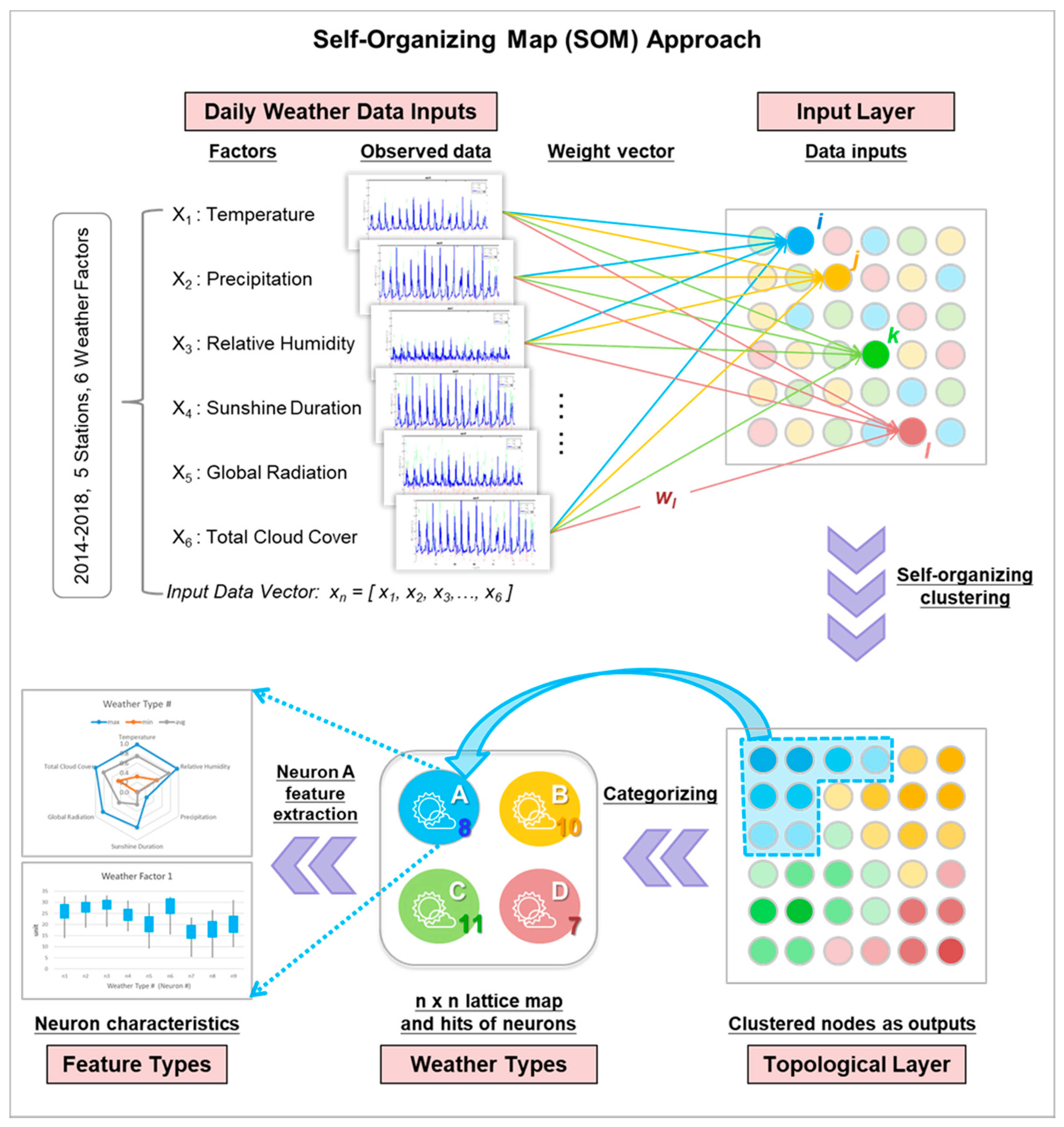
Figure 2 illustrates the concept of the SOM approach in this research. The datasets were input into the SOM network for clustering according to weather similarities by calculating the differences, namely, the distances, between every two inputs on the multi-dimensional topology. The shortest distance (i.e., the minimal difference) between any two inputs indicates that they share more resembling weather characters than others; therefore, they are grouped into one category (i.e., one neuron). Weather features may be clustered into various categories (neurons) depending on the research purposes. Given relatively limited differences in terms of geographical distance among the five weather stations and environmental conditions in northern Taiwan, the variation in weather features may not be too drastic; therefore, this study determined the network size of the SOM to be 3 × 3 (= 9 categories of weather types in total).
In reference to the traditional Chinese Farmers’ Calendar, the concept of a “10-day period”, also called the “xun” in Chinese, has been commonly used as a temporal cycle for planning and engaging cultivation tasks in Chinese society. There are basically three 10-day periods in a month. With variations of week numbers and start/end dates in a month every year, as well as month/seasons, it is relatively complicated to specify the same period in a year for the analysis and comparison of weather types/features and generalizing weather features over very long temporal periods. Therefore, following the agricultural tradition in Taiwan, the 10-day period was adopted to be the conveniently unified and appropriate temporal scale in this research. Therefore, this research considered the 10-day period to be the temporal scale. The software that was used to run the SOM in this research was MATLAB version 2019b.
3. Results
The strength of an SOM is the ability to directly use uncompressed data rather than only using traditional statistics with diluted weather attributes or converting them into certain performance indicators [63]. SOM also effectively provides a means to visualize the complex distribution of weather features to classify and reveal the synoptic weather patterns and attributes of the temporal sequence over a region of interest. In this research, the SOM led to two outcomes for further analysis: first, the result of nine weather feature types (neurons) at each weather station in northern Taiwan, and second, the distribution of weather types throughout the years at the specific weather station indicated the temporal trend/pattern of local weather features. These two results are delineated as follows.
3.1. Types of Weather Features
Figure 3 illustrates the SOM results. Figure 3a shows the number of datasets in each SOM neuron that represented similar features. Figure 3b shows the numbering labels that were associated with the neurons of the SOM topological map. It is evident that neurons #2, #3, #4, and #7 accounted for 64% of the total inputs; therefore, these four neurons were the most representative types to depict the overall weather characteristics in northern Taiwan.
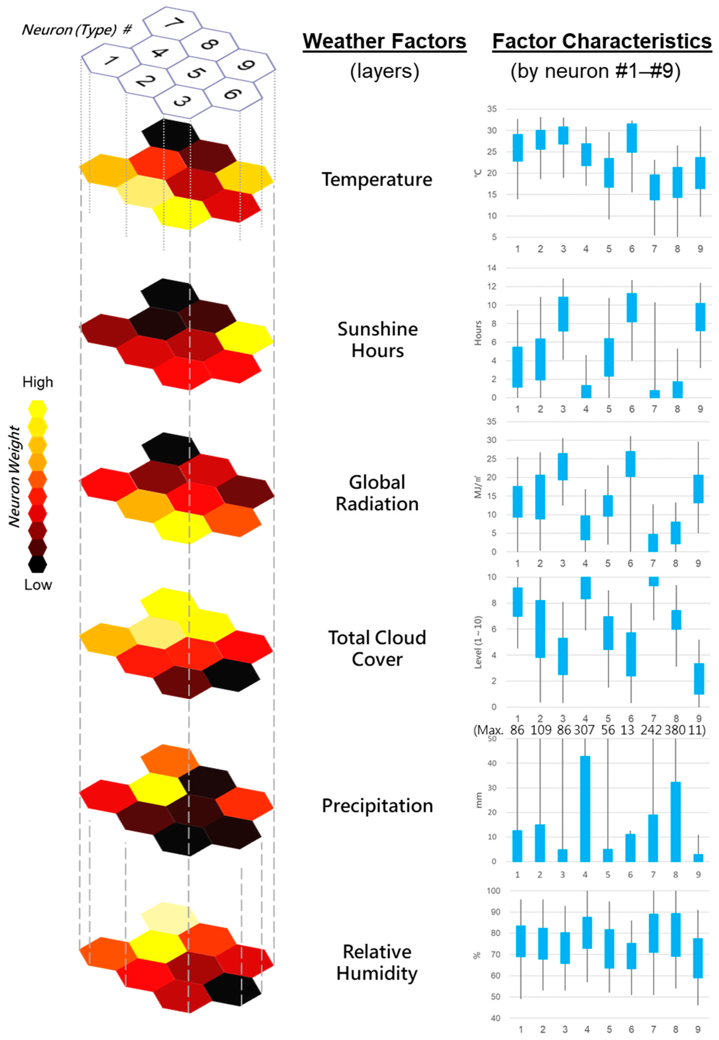
Figure 4 presents the heatmap of the SOM results, indicating the weather-type configuration that can be considered to be the six stratified layers of weather factors with the corresponding characteristics. Every neuron was held at the same position across all weather factor layers so that similar heatmaps in different factor planes represent a high correlation of features. On each weather factor layer, every neuron is shaded in a specific color with a spectrum from light to dark to indicate the weight significance from the highest (in yellow) to the lowest (in black). Therefore, each heatmap represents the feature intensity of a weather factor learned by the SOM. The four corners of the SOM can thus be taken as the most extreme nodes in terms of climate variability, with a smooth continuum in between [60]. All data inputs that were assigned in each neuron for each weather factor layer were extracted to further explore their typical characteristics in common via statistics methods, where the characteristics of each weather factor are illustrated in the form of a stock chart. They are visually presented to show the significance and variation of each specific weather factor in each neuron in this research. With the neuron labels (#1–#9) on the horizontal axis, each blue rectangle comprises the ranges of average value plus/minus one standard deviation of all data in that specific neuron. The top and bottom tips of black vertical lines indicate the maximum and minimum values of all data in that specific neuron, respectively. It is noted that in the precipitation layer, the enormous values of the maximum rainfalls are labeled directly on top so that the precipitation variation is still visually explicit.
Among all nine neurons, the temperature weighed most significantly (the highest value) in neuron #3, then followed by neurons #2, #9, #1, and #4 accordingly with gradually darker colors, and lastly, neuron #7 in black denoted the lowest value. As for the total cloud cover layer, neurons #6 and #3 on the lower-right presented the least cloud cover (i.e., the sunniest condition), then neurons #2, #5, and #9 followed with gradually higher temperatures toward the upper-left, and neuron #7 in yellow denoted the most cloudy condition (i.e., least sunny).
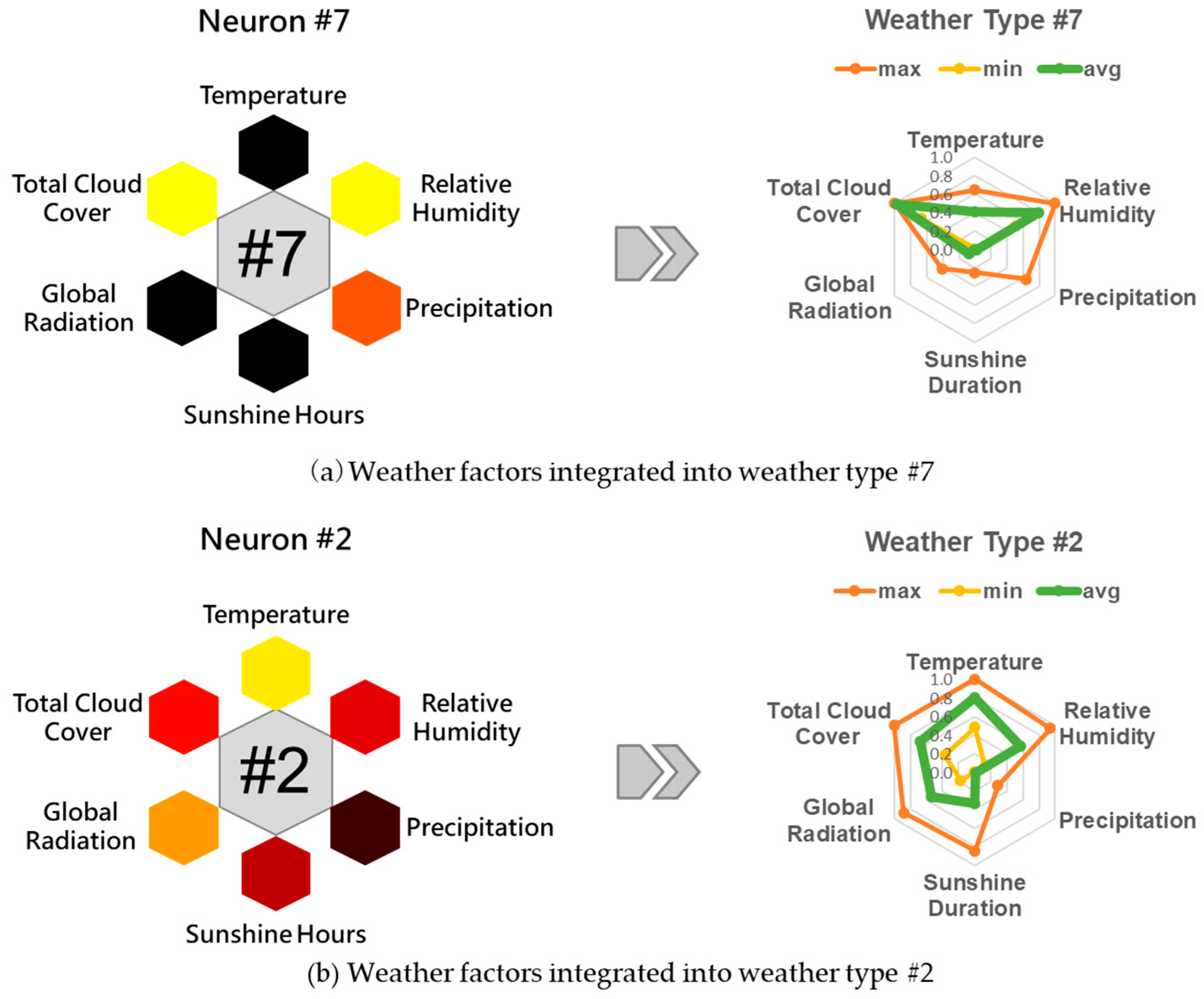
Therefore, through integrating the characteristics of the six weather factors with various significances allocated, each neuron designated one type of weather feature. Since neurons #7 and #2 comprised the two most significant inputs, they were taken to illustrate how the six weather factors are transformed into a radar diagram of each weather type and what their overall features were, as shown in Figure 5.
In neuron #7, the temperature, sunshine hours, and global radiation factors were all colored black, indicating these three factors displayed the lowest levels. In contrast, relatively high humidity and total cloud cover appear (in yellow), suggesting that these factors displayed the highest levels. Precipitation was orange, meaning it displayed a medium level. As a consequence, neuron #7, which was also denoted as weather type #7, integrated the weather characteristics of the lowest temperature, the highest humidity, medium rainfall, the least sunshine hours, the lowest global radiation, and the highest total cloud cover, which complied with the general weather phenomena in winter from our observation (Figure 5a). With the same rationale, neuron #2 exemplified the weather characteristics of high temperature, medium humidity, and low precipitation, along with lower sunshine hours, high global radiation, and lower total cloud cover (Figure 5b).
When converting the above results of neuron #2 to the radar diagram shown in Figure 5b, the green line linking the green points (average values) formed the “shape of type #2 in terms of average values”. The same rationale applied to the orange points and line, denoting the “shape of type #2 in terms of the maximum values”, as well as to the yellow ones, denoting the “shape of type #2 in terms of the minimum values”. Therefore, the daily average, maximum, and minimum records for each weather type were delineated explicitly. Overall, type #2 indicated that the maxima of temperature, relative humidity, and total cloud cover reached the highest level of 1.0 at the outmost edge on the hexagon, while the sunshine hours and global radiation positions were at 0.8 (the second-highest level) and precipitation positions were at 0.2 (a very low level). The “shape of the average values” profiled the dominant weather factors, which were temperature, humidity, and total cloud cover positioning in the range 0.6–0.8. The other three factors played much less significant roles, where precipitation, sunshine hours, and global radiation positioning were at around 0.0, 0.4, and 0.6, respectively.
3.2. Weather Pattern at Five Stations in Northern Taiwan
This research originally explored the weather features from five stations in northern Taiwan, where Table 2 illustrates the integrated results. Each station presented its own weather characteristics, but overall, types #2, #3, #4, #7, and #9 were the most typical ones at the Banqiao, Taipei, and Xinwu stations, while Tamshui and Keelung presented their own types of weather features. The seasonal characteristics of weather features at the other four stations also deserve more elaboration in the form of the comprehensive analysis that was given for the Taipei Station in this research.
3.3. Temporal Pattern of Weather Types
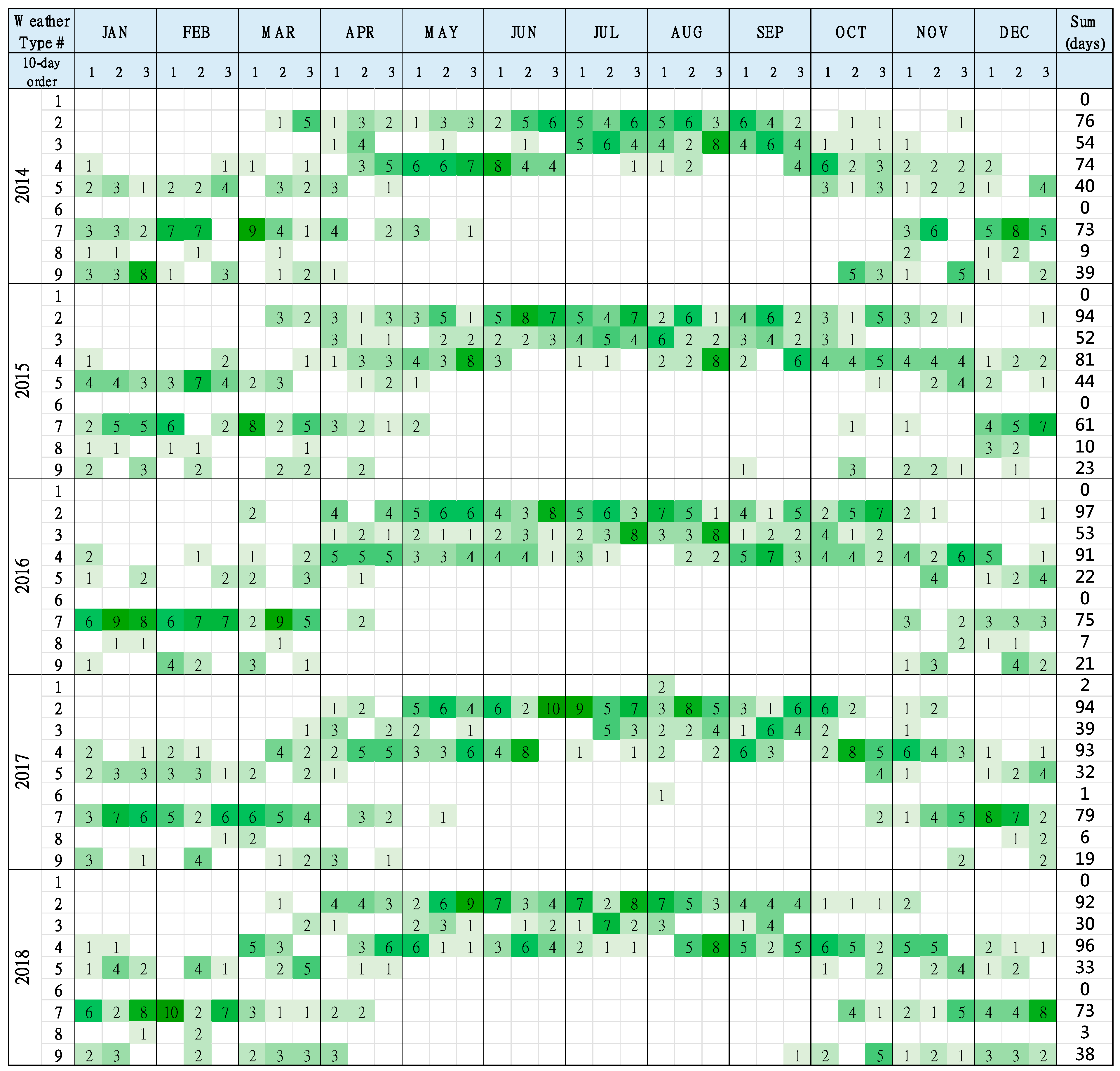
The result of the Taipei weather station is taken as the main focus for elaboration in this research. Figure 6 shows the occurrences (counts) of the nine weather types on a 10-day basis from 2014 to 2018. Each cell is visually shaded with a color spectrum indicating the frequency intensification. The higher the occurrence frequency is, the darker the cell color is. Therefore, the occurrence time, frequency, and duration of each weather type are presented explicitly on the pattern of weather types that occurred at specific weather stations throughout the years between 2014 and 2018.
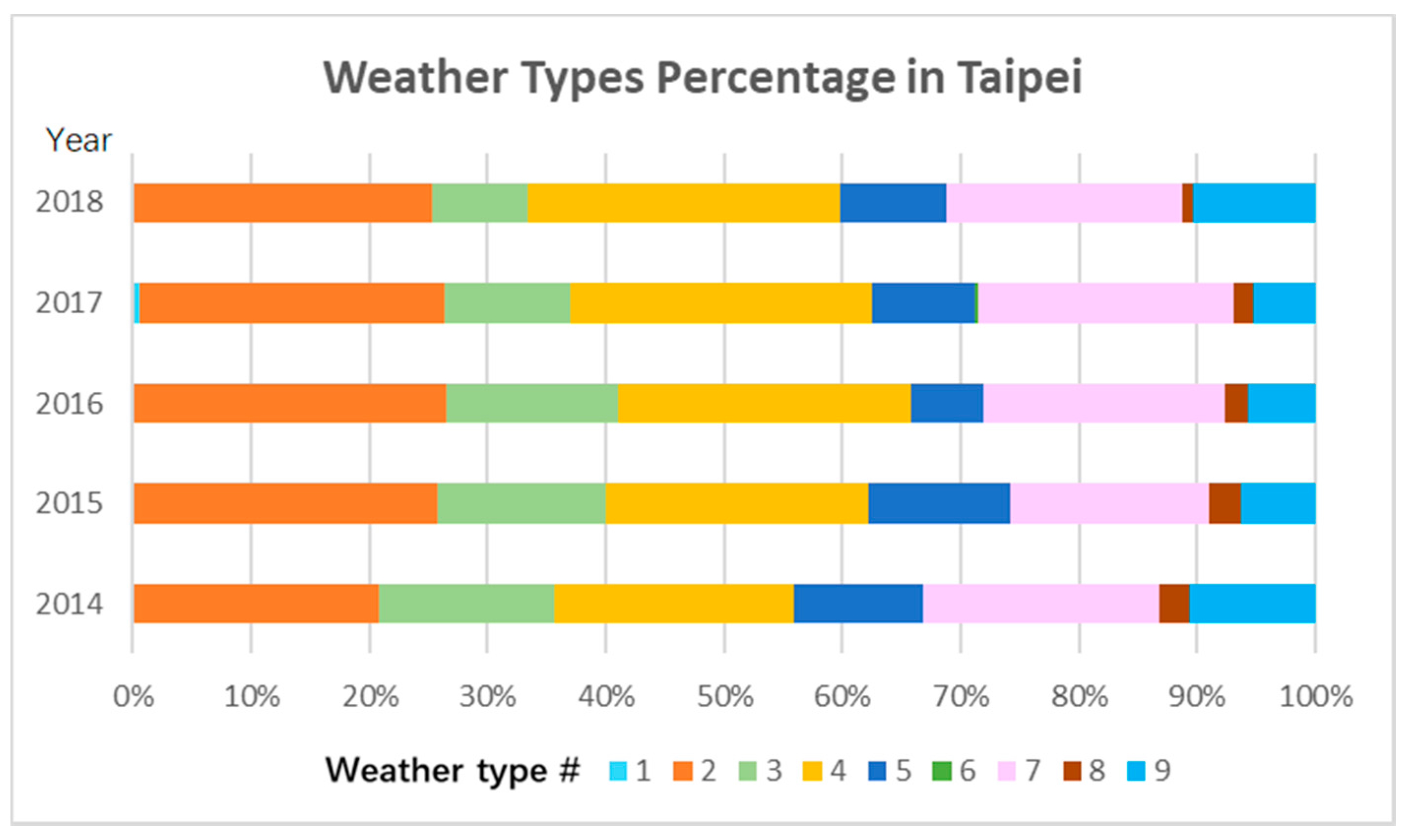
Figure 7 shows the percentage of each weather type that occurred on an annual basis. Figure 6 and Figure 7 explicitly display that there was a stable trend and similar occurrence percentages for the variation of weather types over the five years. Though the annual occurrences of each weather type might be slightly different and/or offset, the timings of the sequential trend and the duration were generally consistent. In this regard, it is essential to examine the high-frequency occurrence distribution, duration, continuity, and extent profiles rather than the forecasts of weather features on specific dates. Therefore, it was reasonable to aggregate the 5-year occurrences under the same 10-day basis into overall seasonal features by summing all the values in each cell to strengthen the significance and distribution of feature types, as illustrated in Figure 8a.
In addition, when the specific weather type lasted continuously (especially with high occurrence frequency) and multiple weather types took place over the same time frame, these weather types could be considered altogether to be the “representing weather features” of the sequential regularity and pattern. In this regard, from the distribution of concentration and continuity, it is explicit that the nine weather types that were distributed throughout the thirty-six 10-day periods formed three distinct sections of temporal groups annually, referring to sections A, B, and C marked with dashed rectangles in Figure 8a.
Section A (marked with a dashed orange rectangle) represented the period from “early spring through late fall” (mainly full summer). Section B (marked with a dashed blue rectangle) represented the period from “mid-fall through next mid-spring” (mainly full winter), with two sub-sections, namely, section B2 from early autumn to winter at the year-end and section B1 from winter at the beginning of the year (1 January) to early summer. Section C (marked with a dashed yellow rectangle) referred to the absent or barely occurring types all year round. There were some overlaps of 10-day periods between sections A and B1, similarly between sections B2 and A. This explained the seasonal alternation with diverse weather types and complex variations during spring and fall.
Figure 8b also delineates the two leading weather types with the associated occurrence percentages summed from major (in pink shades) and secondary (in yellow shades) weather types in each 10-day period. With shaded cells indicating that the percentage exceeded the designated one listed in the sum column, this demonstrates how significant and representative the weather type was in each 10-day period. In addition, the last row shows the subtotal percentage of the two leading types, together with over 60% (in green shades) as a high concentration and continuum of occurrences. The 10-day periods without green shaded cells represent the percentage <60% as non-leading major and secondary occurrences, which also refers to more diverse and variant weather types taking place in springs and falls as the seasonal transition.
3.4. Frequency, Duration, and Distributions of Type Occurrences
The collective occurrences of the nine weather types at Taipei Station were analyzed from two perspectives: the features and distribution of occurring types and the comprehensive outcome during designated timespans (season, month, and 10-day periods), which are elaborated in the following.
Figure 8a illustrates that among all nine feature types, types #2 (25.8%), #4 (24.7%), and #7 (19.8%) were the main weather types at the Taipei Station and altogether accounted for 70.3% of the occurrences out of the occurrences of all types over the five years. There were barely any type #1 or #6 weather patterns each year.
Figure 9 illustrates the occurrence distribution and duration of types in sections A, B, and C. Section A in Figure 9a basically spanned from April to early October, where the highest frequency weather types were types #2 (red bar), #4 (green bar), and #3 (yellow bar), implying they are the representative weather types during the season from mid-spring to early fall. These types tended to appear sporadically or were absent before April and disappeared gradually after mid-October till the year-end. The occurrence timespans and high frequencies of types #2 and #4 seemed complementary to each other, with one rising (appearing) and the other falling (disappearing), while type #3 peaked shortly in the hottest days of mid-summer (mid-July to mid-September). Section B in Figure 9b, on the other hand, shows the duration starting from mid-October to the next late April (covering late fall, winter, and the following spring), with a gradual transition through types #4, #7, #5, and #9. There were barely any type #1 or #6 weather patterns, with only 1–2 occurrences in early August in Section C.
3.5. Main Features of Weather Types in Taipei City
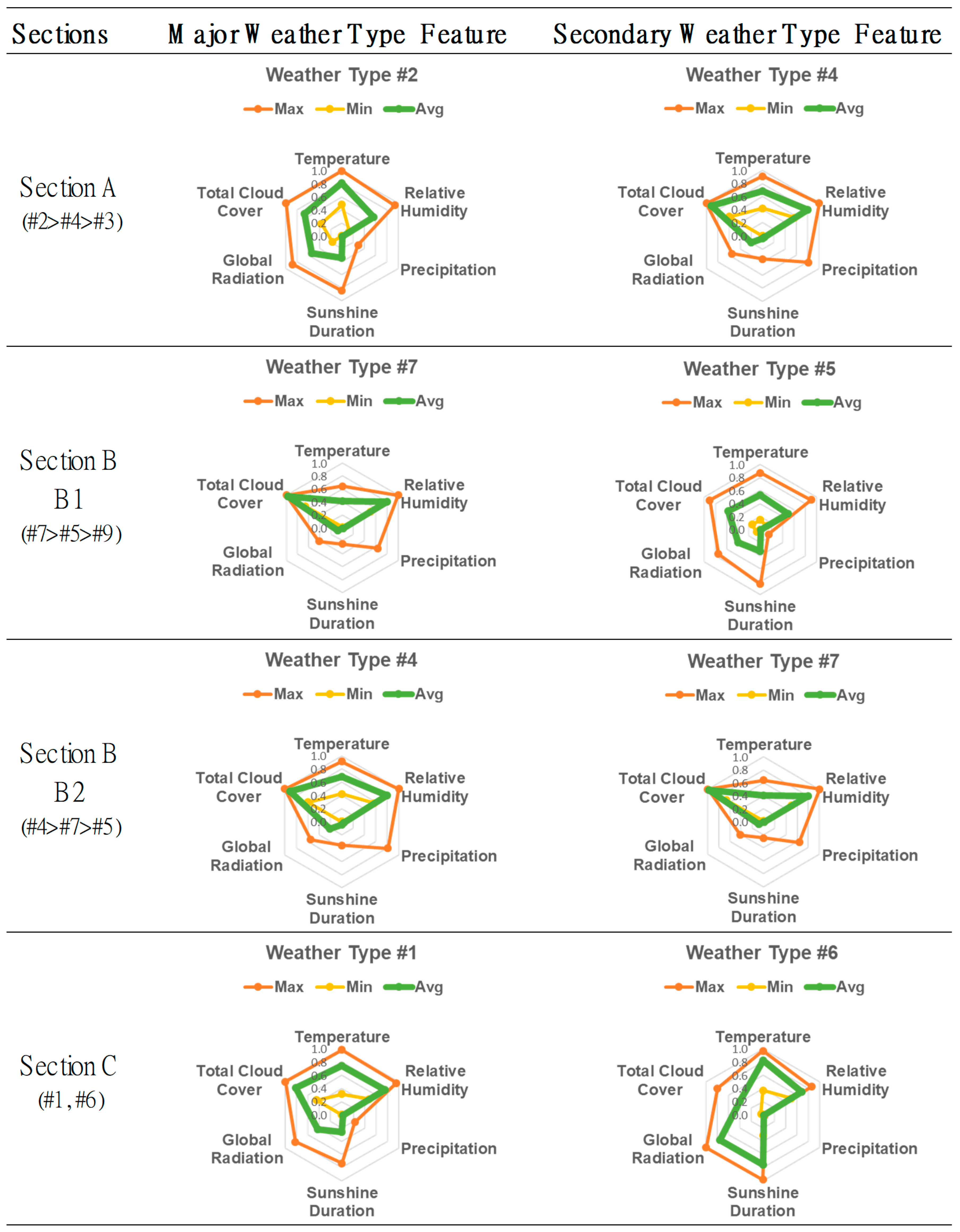
To elaborate the weather types and features in the Taipei area for further application to UA, Figure 10 highlights the features of the two leading weather types for sections A, B, and C to visually present the variations of the six weather factors during the designated period.
Comprehensively, with cross-referencing to Figure 8, Figure 9 and Figure 10, the annual weather pattern in the Taipei area presented the following features in the sequential timing of a year are elaborated as follows.
Though mainly concentrating from April to mid-June and from mid-August to November (before and after summer), type #4 weather patterns occurred in almost every 10-day period throughout 2014–2018. This was taken as the basic annual weather feature in Taipei.
Intensifying from January to March and in December, type #7 weather patterns dominated the weather features in winter, with the lowest temperature range (14–20 °C), little rainfall, high humidity (80%), the least global radiation (0–5 MJ/m2) and sunshine hours, the highest level of cloud cover of the year, and sometimes accompanied by the second most frequent weather pattern, namely, type #5, with its relatively mild/less “winter touch” features.
During the periods of March–April (spring) and October–November (fall), all the weather types, except for types #1 and #6, appeared alternatively, indicating greater variations and less stable features, for instance, temperature (14–31 °C), precipitation (15–43 mm), global radiation (0–26 MJ/m2), sunshine duration (0.5–11 h), and cloud cover (levels 1–10). Types #7 (winter) and #5 played the most significant roles and frequently occurred in early March and then gradually disappeared, followed by types #4 and #2, mainly from April (as the summer began to emerge). Such weather features proceeded in a mirrored way from October to November as winter approached.
From May to September (late spring through summer to early fall), types #2 and #4 occur were dominant and alternated, with their high temperature (25–30 °C), little precipitation, and large variation in global radiation, sunshine hours, and cloud cover. Furthermore, accompanied with a slight trace of type #3, the summer feature reached its climax occurrences, with the highest temperature (27–31 °C), very limited rainfall, the most abundant global radiation (19–26 MJ/m2) and sunshine hours (7–11 h), the least rainfall, and lower cloud cover (levels 2.5–5) in the summer peak from mid-July to September. Then, from October, the weather feature returned gradually to the basic type (type #4) and transformed into fall–winter patterns.
4. Discussion
Weather classification of typical local weather features from past experiences and historical data can greatly enhance agricultural decision making by identifying the timings for effective cultivation activities and the corresponding efficiency of resource use. For example, the statistics of the historical average, maximum, and minimum of certain weather factors (e.g., temperature and precipitation) within a time interval (month or year) provides a very rough idea of the local weather condition with variation ranges. In addition, some specific daily phenomena with the presence of various weather factors occurred frequently and repetitively during a certain period in a year; therefore, such alternation of seasonal features can be considered to be the “typical weather patterns” and is expected to continue in the following years. This section discusses and extends the use of SOM, weather types, and features and particularly focuses on the potential application of the feature results.
4.1. SOM Approach Contributions to the Weather Typing
The results of the weather features from the SOM approach can effectively excavate out more hidden details of characteristics on the key weather types. It explicitly visualizes the weather patterns and trends in terms of their occurring time, frequency, intensity, distribution, duration, and transition nexus with various types. Furthermore, it is rational to elucidate/interpret what weather types are likely to occur during designated periods of interest and how meteorological factors are expected to appear substantially. Therefore, it is practical to grasp the temporal distribution and seasonal changes of weather features to plan for appropriate strategies and measures when necessary.
4.2. Potential Applications
The investigation of weather features and historical meteorological data throughout the year can be a reference for agricultural decisions in various cultivation activities, such as species selection, planting, harvesting, transplanting, defoliation, fertilization, and irrigation [11]. In addition, necessary precautions can be further adopted to preempt crop stress control, sheltering, disease risk reduction, and pest control, as well as to explore sustainable resource mechanisms in terms of collection, storage, and utilization.
The symbolic representation of temporal weather features is the key to effective crop planting plans that suggest farmers take necessary actions and measures for optimal crop growing and harvesting, with more efficient resource utilization and protection from potential weather damage. For example, the timings of meteorological conditions of temperature, precipitation, and sunshine hours affect crop-growing schedules regarding seeding, seedling, flowering, fruiting, and harvesting, particularly through the necessary heat for succession, water supply for irrigation, and sunlight exposure for photosynthesis. Therefore, the understanding of the temporal distribution and intensity of local weather types would contribute to enhancing the cropping (such as the species selection) under favorable weather, with adequate supporting facilities being installed when necessary (such as the provision of shade for crops from sunscald and increasing ventilation to prevent against potential insects/disease due to high temperature and humidity).
The features of weather types can also enhance the prediction of rainwater and solar power output by calculating the related green resources input based on meteorology for cultivation during the process of species selection, maintenance, and resources regulation regarding collection, storage, and provision. Particularly for urban agriculture via rooftop farming and community gardening, the water and electricity that are needed for irrigating farms often come from public utilities. Hence, drawing practical planting plans and operation strategies by taking advantage of favorable weather features during designated periods for specific measurements/adaptations can be sustainable. For instance, installing an external rainwater tank and solar power facility, as well as prioritizing the use of rainfall and sunlight as green/renewable resources for efficient collection, storage, and reuse for farming irrigation, reduces the dependence on tap water and municipal electricity.
The Da-an rooftop farm with elevated planters extensively laid out on its rooftop can be taken as a study site for the application of weather types and features that are relevant to UA activities. The selection of crop species and some auxiliary measurements are proposed as application examples in the following.
Sweet potato leaves (SPL) (Ipomoea batatas (L.) Lam.) has been one of the commonly planted species at the Da-an site over the years. As popular leafy vegetables, SP is a subtropical herbaceous trailing vine with a relatively short growing cycle to produce frequent harvests during growing seasons; it requires continuous heat, abundant daily watering (with good drainage), long sunlight exposure, and is very sensitive to chilly temperatures [64]. SPL prefers cooler and drier seasons as seedlings, then it can mature fast in hot and humid months (with a favorable optimal temperature range between 20–30 °C). SP leaves can be picked for harvest within as short as 18 days in hot summers but as long as 30 days in cold winters [65]. According to the analysis of major weather types that were developed for Taipei in this research, SPL can serve as a very good species that is suitable to grow under the weather conditions in Taipei, and its most favorable growing seasons would fall within section A. By referring to Figure 4, Figure 8 and Figure 10, with SPL seedlings planted in April, they can grow prosperously from May to September when weather types #2 and #4 are dominant (with characteristics of high temperature (25–30 °C); constantly high humidity; limited daily precipitation but sometimes showers up to over 300 mm; and large variations in global radiation, sunshine hours, and cloud cover). It is noted that type #3 is concentrated from mid-July to mid-September (with characteristics of very hot days, reaching the highest temperature (27–31 °C), sunshine hours (7–11 h daily), and radiation (19–26 MJ/m2). SPL grows slowly from November to next February, during which, weather types transform gradually from types #4 to #7 with winter characteristics. In other words, as seen in Figure 4 and Figure 8b, the total occurrence frequency of weather types #2, #3, and #4 accounted for 72–95% in section A starting from late April to the end of September. Therefore, SPL would enjoy the high temperature and humidity, as well as the long sunshine hours and strong radiation, with some fluctuation between these three weather types.
With types #2, #3, and #4 occurring alternately during section A, cross-referencing between Figure 4, Figure 8, and Figure 9, types #2 and #3 featured low daily precipitation (12–15 mm) whereas type #4 featured high daily precipitation (42 mm). Furthermore, all three types had occasional extremely high daily precipitation (with a maximum of up to 86–307 mm). These showed that there were potential demands to set up provisional rainwater tanks, such as additional water containers and large inclined planes to increase rainwater collection areas and storage volume as watershed during intensive showers, which could be set aside for later irrigation in a sustainable way. Therefore, by way of providing an SPL irrigation plan to satisfy SPL’s abundant water needs in hot summers, the daily irrigation water supply can be managed to come from an additional setup of a rainwater tank to collect and store torrential rain as a supplement to irrigation water from May to September, specifically during section A. The potential size of the suggested rainwater tank depends on the SPL planting area, the number of plants, and the loading capacity of the rooftop of the building.
The sunshine duration can affect plants’ growth due to sunlight exposure for photosynthesis; therefore, some crop species prefer longer sunlight exposure to grow prosperously than others. The features of sunshine duration, global radiation, and total cloud cover level can also impact the efficiency of solar power utilization. Therefore, seasons with long sunshine hours and radiation (type #3) showed higher suitability for heliophyte species or require some shading facility for sciophyte species to prevent sunscald. On the other hand, this also suggests the great potential to establish a solar power facility for providing green energy to the automatic irrigation system in the farm.
5. Conclusions
This study proposed an SOM neural network to cluster and identify the specific features of weather types based on six meteorological variables at five weather stations in northern metropolitan Taiwan. The daily meteorological datasets, comprising temperature, precipitation, relative humidity, sunshine duration, global radiation, and total cloud cover from 2014–2018, were collected as inputs to the SOM network and then were classified into a topological map based on the similarities of weather features to investigate their multi-collinear relationships for spatiotemporal distribution analysis.
The results of the weather features from the SOM classification not only corresponded to what we know about the general weather features in the five metropolitan areas but also provided detailed and integrated information of weather features on the occurrence period, duration, frequency, intensity, and variation range from historical data sets on a 10-day basis. This study contributes to the practicability for urban agriculture planning by exploring the in-depth weather features in northern Taiwan to conduct urban farming in planting arrangement, installing equipment, and managing the crop-growing process (seeding, seedling, growth rate, maturing, flowering, fruiting, harvesting, etc.) in response to local weather features before launching planting in the five study areas.
The results of this study can also be applied to selecting appropriate species for planting in favorable seasons with appropriate weather features. The size of the rainwater tank and the scale of solar power equipment can also be identified to comply with weather features to achieve the optimal resource utilization efficiency to grow and irrigate vegetables so as to reduce the municipal water and electricity use during farming operations.
Given the arising phenomenon of climate change, the chances of unprecedented weather with continuous hot/chilly days, rainstorms, and droughts tend to occur more frequently. However, such weather conditions were not included in the weather typing in this research because outlier data (especially for extremely high precipitation, which is mostly caused by typhoons or sudden torrential rains) were removed at the data preprocessing stage. It is suggested that the extreme weather events in cities of northern Taiwan require further investigation regarding their occurrence time and frequency, as well to help with providing advice as a further reference/strategy for urban agriculture operations if possible so that more risks may be anticipated and stronger adaptation measures could be prepared.
Author Contributions
Conceptualization, A.H. and F.-J.C.; methodology, A.H. and F.-J.C.; software, A.H.; validation, A.H. and F.-J.C.; formal analysis, A.H.; investigation, A.H.; resources, A.H. and F.-J.C.; data curation, A.H.; writing—original draft preparation, A.H.; writing—review and editing, A.H. and F.-J.C.; visualization, A.H.; supervision, F.-J.C.; project administration, F.-J.C.; funding acquisition, F.-J.C. All authors have read and agreed to the published version of the manuscript.
Funding
This study was supported by the Ministry of Science and Technology, Taiwan (grant number: 107-2621-M-002-004-MY3), and the Chi-Seng Water Management Research and Development Foundation, Taipei.
Institutional Review Board Statement
Not applicable.
Informed Consent Statement
Not applicable.
Data Availability Statement
The data presented in this study are available from the Taiwan Central Weather Bureau website.
Acknowledgments
The datasets provided by the CWB, Taiwan, are acknowledged. The authors would also like to thank the editors and anonymous reviewers for their constructive comments that greatly contributed to enriching the manuscript.
Conflicts of Interest
The authors declare no conflict of interest.
References
- FAO. Urban and Peri-Urban Agriculture, IV. Characteristics of Urban and Peri-Urban Agriculture. 2020. Available online: http://www.fao.org/unfao/bodies/coag/coag15/x0076e.htm (accessed on 21 September 2021).
- Da Cruz, S.M.S.; Steglich, A.; Cruz, P.V.; Vieira, A.C.M. Investigating the challenges and opportunities of urban agriculture in global north and global south countries. In Frontiers of Science and Technology: Reports on Technologies for Sustainability–Selected Extended Papers from the Brazilian-German Conference on Frontiers of Science and Technology Symposium (BRAGFOST); Kanoun, O., Viehweger, C., Eds.; Walter de Gruyter GmbH & Co. KG: Berlin, Germany, 2017; pp. 95–110. [Google Scholar]
- Badami, M.G.; Ramankutty, N. Urban agriculture and food security: A critique based on an assessment of urban land constraints. Glob. Food Sec. 2015, 4, 8–15. [Google Scholar] [CrossRef]
- Pearson, L.J.; Pearson, L.; Pearson, C.J. Sustainable urban agriculture: Stocktake and opportunities. Int. J. Sustain. Agric. Res. 2010, 8, 7–19. [Google Scholar] [CrossRef]
- Specht, K.; Schimichowski, J.; Fox-Kämper, R. Multifunctional Urban Landscapes: The Potential Role of Urban Agriculture as an Element of Sustainable Land Management. In Sustainable Land Management in a European Context. Human-Environment Interactions; Weith, T., Barkmann, T., Gaasch, N., Rogga, S., Strauß, C., Zscheischler, J., Eds.; Springer: Basel, Switzerland, 2021; Volume 8, pp. 291–303. [Google Scholar]
- Ellis, F.; Sumberg, J. Food production, urban areas and policy responses. World Dev. 1998, 26, 213–225. [Google Scholar] [CrossRef]
- Zezza, A.; Tasciotti, L. Urban agriculture, poverty, and food security: Empirical evidence from a sample of developing countries. Food Policy 2010, 35, 265–273. [Google Scholar] [CrossRef]
- Barrios, S.; Ouattara, B.; Strobl, E. The impact of climatic change on agricultural production: Is it different for Africa? Food Policy 2008, 33, 287–298. [Google Scholar] [CrossRef] [Green Version]
- Agnolucci, P.; Rapti, C.; Alexander, P.; De Lipsis, V.; Holland, R.A.; Eigenbrod, F.; Ekins, P. Impacts of rising temperatures and farm management practices on global yields of 18 crops. Nat. Food 2020, 1, 562–571. [Google Scholar] [CrossRef]
- Das, H.P.; Doblas-Reyes, F.J.; Garcia, A.; Hansen, J.; Mariani, L.; Nain, A.S.; Ramesh, K.; Rathore, L.S.; Venkataraman, R. Chapter 5: Weather and climate forecasts for agriculture. Guide to agricultural, meteorological practices. In Guide to Agricultural Meteorological Practices, 2010 ed.; Gommes, R., Challinor, A., Das, H., Dawod, M.A., Mariani, L., Tychon, B., Trampf, W., Eds.; WMO: Geneva, Switzerland, 2012; Available online: https://library.wmo.int/doc_num.php?explnum_id=3996 (accessed on 22 October 2021).
- Frisvold, G.B.; Murugesan, A. Use of weather information for agricultural decision making. Weather Clim. Soc. 2013, 5, 55–69. [Google Scholar] [CrossRef]
- Haigh, T.; Takle, E.; Andresen, J.; Widhalm, M.; Carlton, J.S.; Angel, J. Mapping the decision points and climate information use of agricultural producers across the US Corn Belt. Clim. Risk Manag. 2015, 7, 20–30. [Google Scholar] [CrossRef] [Green Version]
- Abhishek, K.; Singh, M.P.; Ghosh, S.; Anand, A. Weather forecasting model using artificial neural network. Procedia Technol. 2012, 4, 311–318. [Google Scholar] [CrossRef] [Green Version]
- Narvekar, M.; Fargose, P. Daily Weather Forecasting using Artificial Neural Network. Int. J. Comput. Appl. 2015, 121, 9–13. [Google Scholar] [CrossRef]
- Liu, J.N.; Hu, Y.; You, J.J.; Chan, P.W. Deep neural network based feature representation for weather forecasting. In Proceedings on the International Conference on Artificial Intelligence (ICAI); The Steering Committee of the World Congress in Computer Science, Computer Engineering and Applied Computing (WorldComp): Las Vegas, NV, USA, 2014; p. 1. [Google Scholar]
- Tran, T.T.K.; Bateni, S.M.; Ki, S.J.; Vosoughifar, H. A Review of Neural Networks for Air Temperature Forecasting. Water 2021, 13, 1294. [Google Scholar] [CrossRef]
- Chiang, Y.M.; Chang, F.J.; Jou, B.J.D.; Lin, P.F. Dynamic ANN for precipitation estimation and forecasting from radar observations. J. Hydrol. 2007, 334, 250–261. [Google Scholar] [CrossRef]
- Francik, S.; Kurpaska, S. The use of artificial neural networks for forecasting of air temperature inside a heated foil tunnel. Sensors 2020, 20, 652. [Google Scholar] [CrossRef] [Green Version]
- Trebing, K.; Mehrkanoon, S. Wind speed prediction using multidimensional convolutional neural networks. In Proceedings of the 2020 IEEE Symposium Series on Computational Intelligence (SSCI), Canberra, Australia, 1–4 December 2020; pp. 713–720. [Google Scholar]
- Chattopadhyay, A.; Hassanzadeh, P.; Pasha, S. Predicting clustered weather patterns: A test case for applications of convolutional neural networks to spatio-temporal climate data. Sci. Rep. 2020, 10, 1317. [Google Scholar] [CrossRef] [PubMed]
- Xiao, H.; Zhang, F.; Shen, Z.; Wu, K.; Zhang, J. Classification of weather phenomenon from images by using deep convolutional neural network. Earth Space Sci. 2021, 8, e2020EA001604. [Google Scholar] [CrossRef]
- Riyazuddin, Y.M.; Basha, S.M.; Reddy, K.K. An approach for prediction of weather system by using back propagation neural network. Int. J. Sci. Dev. Res. 2017, 2, 117–121. [Google Scholar]
- Kakar, S.A.; Sheikh, N.; Naseem, A.; Iqbal, S.; Rehman, A.; Kakar, A.U.; Kakar, B.A.; Kakar, H.A.; Khan, B. Artificial neural network based weather prediction using Back Propagation Technique. Int. J. Adv. Comput. Sci. Appl. 2018, 9, 462–470. [Google Scholar] [CrossRef]
- Wica, M.; Witkowsk, M.; Szumiec, A.; Ziebura, T. Weather forecasting system with the use of neural network and backpropagation algorithm. In Proceedings of the International Conference on Data Engineering and Communication Technology; Springer: Singapore, 2019; Volume 2468, pp. 37–41. [Google Scholar]
- Chang, F.J.; Chang, L.C.; Kao, H.S.; Wu, G.R. Assessing the effort of meteorological variables for evaporation estimation by self-organizing map neural network. J. Hydrol. 2010, 384, 118–129. [Google Scholar] [CrossRef]
- Chang, L.C.; Wang, W.H.; Chang, F.J. Explore training self-organizing map methods for clustering high-dimensional flood inundation maps. J. Hydrol. 2021, 595, 125655. [Google Scholar] [CrossRef]
- Reddy, P.C.; Sureshbabu, A. An adaptive model for forecasting seasonal rainfall using predictive analytics. Int. J. Intell. Syst. 2019, 12, 22–32. [Google Scholar] [CrossRef]
- Wu, C.L.; Chau, K.W. Prediction of rainfall time series using modular soft computing methods. Eng. Appl. Artif. Intell. 2013, 26, 997–1007. [Google Scholar] [CrossRef] [Green Version]
- Taormina, R.; Chau, K.W. ANN-based interval forecasting of streamflow discharges using the LUBE method and MOFIPS. Eng. Appl. Artif. Intell. 2015, 45, 429–440. [Google Scholar] [CrossRef]
- Wang, W.; Du, Y.; Chau, K.; Chen, H.; Liu, C.; Ma, Q. A Comparison of BPNN, GMDH, and ARIMA for Monthly Rainfall Forecasting Based on Wavelet Packet Decomposition. Water 2021, 13, 2871. [Google Scholar] [CrossRef]
- Ruß, G.; Kruse, R.; Schneider, M.; Wagner, P. Visualization of agriculture data using self-organizing maps. In Applications and Innovations in Intelligent Systems XVI. SGAI 2008; Allen, T., Ellis, R., Petridis, M., Eds.; Springer: London, UK, 2008; pp. 47–60. [Google Scholar]
- Ponmalai, R.; Kamath, C. Self-Organizing Maps and Their Applications to Data Analysis; (No. LLNL-TR-791165); Lawrence Livermore National Lab.: Livermore, CA, USA, 2019. [Google Scholar]
- Chang, F.J.; Chang, L.C.; Kang, C.C.; Wang, Y.S.; Huang, A. Explore spatio-temporal PM2. 5 features in northern Taiwan using machine learning techniques. Sci. Total Environ. 2020, 736, 139656. [Google Scholar] [CrossRef] [PubMed]
- Doan, Q.V.; Kusaka, H.; Sato, T.; Chen, F. A structural self-organizing map algorithm for weather typing. Geosci. Model Dev. 2021, 14, 2097–2111. [Google Scholar] [CrossRef]
- Hidalgo, D.R.; Cortés, B.B.; Bravo, E.C. Dimensionality reduction of hyperspectral images of vegetation and crops based on self-organized maps. Inf. Process. Agric. 2021, 8, 310–327. [Google Scholar] [CrossRef]
- Liu, Y.; Weisberg, R.H. A review of self-organizing map applications in meteorology and oceanography. In Self-Organizing Maps: Applications and Novel Algorithm Design; Mwasiagi, J.I., Ed.; IntechOpen: Rijeka, Croatia, 2011; Volume 1, pp. 253–272. Available online: https://www.intechopen.com/chapters/13302 (accessed on 23 February 2020). [CrossRef] [Green Version]
- Taşdemir, K.; Wirnhardt, C. Neural network-based clustering for agriculture management. EURASIP J. Adv. Signal Process 2012, 1, 1–13. [Google Scholar] [CrossRef]
- Satizábal, H.; Barreto-Sanz, M.; Jiménez, D.; Pérez-Uribe, A.; Cock, J. Enhancing decision-making processes of small farmers in tropical crops by means of machine learning models. In Technologies and Innovations for Development; Springer: Paris, France, 2012; pp. 265–277. [Google Scholar]
- Mohan, P.; Patil, K.K. Deep learning based weighted SOM to forecast weather and crop prediction for agriculture application. Int. J. Intell. Eng. Syst. 2018, 11, 167–176. [Google Scholar] [CrossRef]
- Rubem, A.P.S.; de Moura, A.L.; de Oliveira, E.; de Mello, J.S.; Alves, L.A.; Tavares, R.S. Productive performance of small peri-urban farms using self-organizing maps and data envelopment analysis. WIT Trans. Ecol. Environ. 2015, 192, 133–145. [Google Scholar]
- Vergni, L.; Todisco, F. Spatio-temporal variability of precipitation, temperature and agricultural drought indices in Central Italy. Agric. For. Meteorol. 2011, 151, 301–313. [Google Scholar] [CrossRef]
- Hewitson, B.C.; Crane, R. Self-organizing maps: Applications to synoptic climatology. Clim. Res. 2002, 22, 13–26. [Google Scholar] [CrossRef]
- Alexander, L.V.; Uotila, P.; Nicholls, N.; Lynch, A. A new daily pressure dataset for Australia and its application to the assessment of changes in synoptic patterns during the last century. J. Clim. 2010, 23, 1111–1126. [Google Scholar] [CrossRef]
- Loikith, P.C.; Lintner, B.R.; Sweeney, A. Characterizing large-scale meteorological patterns and associated temperature and precipitation extremes over the northwestern United States using self-organizing maps. J. Clim. 2017, 30, 2829–2847. [Google Scholar] [CrossRef]
- Borah, N.; Sahai, A.; Chattopadhyay, R.; Joseph, S.; Abhilash, S.; Goswami, B. A self-organizing map–based ensemble forecast system for extended range prediction of active/break cycles of Indian summer monsoon. J. Geophys. Res. Atmos. 2013, 118, 9022–9034. [Google Scholar] [CrossRef]
- Chang, L.C.; Shen, H.Y.; Chang, F.J. Regional flood inundation nowcast using hybrid SOM and dynamic neural networks. J. Hydrol. 2014, 519, 476–489. [Google Scholar] [CrossRef]
- Chang, L.C.; Chang, F.J.; Yang, S.N.; Tsai, F.H.; Chang, T.H.; Herricks, E.E. Self-organizing maps of typhoon tracks allow for flood forecasts up to two days in advance. Nat. Commun. 2020, 11, 1983. [Google Scholar] [CrossRef] [Green Version]
- Cavazos, T. Using self-organizing maps to investigate extreme climate events: An application to wintertime precipitation in the Balkans. J. Clim. 2000, 13, 1718–1732. [Google Scholar] [CrossRef]
- Cassano, E.N.; Glisan, J.M.; Cassano, J.J.; Gutowski, W.J., Jr.; Seefeldt, M.W. Self-organizing map analysis of widespread temperature extremes in Alaska and Canada. Clim. Res. 2015, 62, 199–218. [Google Scholar] [CrossRef]
- Gibson, P.B.; Perkins-Kirkpatrick, S.E.; Uotila, P.; Pepler, A.S.; Alexander, L.V. On the use of self-organizing maps for studying climate extremes. J. Geophys. Res. Atmos. 2017, 122, 3891–3903. [Google Scholar] [CrossRef]
- Fassnacht, S.R.; Derry, J.E. Defining similar regions of snow in the Colorado River Basin using self-organizing maps. Water Resour. Res. 2010, 46, W04507. [Google Scholar] [CrossRef]
- Hsu, K.C.; Li, S.T. Clustering spatial–temporal precipitation data using wavelet transform and self-organizing map neural network. Adv. Water Resour. 2010, 33, 190–200. [Google Scholar] [CrossRef]
- Zhang, W.; Wang, J.; Jin, D.; Oreopoulos, L.; Zhang, Z. A deterministic self-organizing map approach and its application on satellite data based cloud type classification. In Proceedings of the 2018 IEEE International Conference on Big Data, Seattle, WA, USA, 10–13 December 2018; pp. 2027–2034. [Google Scholar]
- Nguyen-Le, D.; Yamada, T.J. Using weather pattern recognition to classify and predict summertime heavy rainfall occurrence over the Upper Nan river basin, northwestern Thailand. Weather Forecast 2019, 34, 345–360. [Google Scholar] [CrossRef]
- Ohba, M.; Sugimoto, S. Differences in climate change impacts between weather patterns: Possible effects on spatial heterogeneous changes in future extreme rainfall. Clim. Dynam. 2019, 52, 4177–4191. [Google Scholar] [CrossRef]
- CWB Observation Data Inquire System. Available online: https://e-service.cwb.gov.tw/HistoryDataQuery/index.jsp (accessed on 1 August 2019).
- World Maps of Köppen−Geiger Climate Classification. Available online: http://koeppen-geiger.vu-wien.ac.at (accessed on 12 July 2021).
- Kohonen, T. A simple paradigm for the self-organized formation of structured feature maps. In Competition and Cooperation in Neural Nets; Springer: Berlin, Heidelberg, 1982; pp. 248–266. [Google Scholar]
- Kohonen, T. Self-Organizing Maps, 3rd ed.; Springer: Berlin, Germany, 2001. [Google Scholar]
- Sheridan, S.C.; Lee, C.C. The self-organizing map in synoptic climatological research. Prog. Phys. Geogr. 2011, 35, 109–119. [Google Scholar] [CrossRef] [Green Version]
- Heikkinen, M.; Poutiainen, H.; Liukkonen, M.; Heikkinen, T.; Hiltunen, Y. Subtraction analysis based on self-organizing maps for an industrial wastewater treatment process. Math. Comput. Simul. 2011, 82, 450–459. [Google Scholar] [CrossRef]
- Lakshminarayanan, S. Application of self-organizing maps on time series data for identifying interpretable driving manoeuvres. Eur. Transp. Res. Rev. 2020, 12, 25. [Google Scholar] [CrossRef]
- Skific, N.; Francis, J. Self-Organizing Maps: A Powerful Tool for the Atmospheric Sciences. In Applications of Self-Organizing Maps; Johnsson, M., Ed.; IntechOpen: Rijeka, Croatia, 2012; Available online: https://www.intechopen.com/chapters/40865#B7 (accessed on 23 February 2020). [CrossRef] [Green Version]
- Welbaum, G.E. Vegetable Production and Practices, 1st ed.; CABI: Boston, MA, USA, 2015. [Google Scholar]
- Huang, A.; Chang, F.J. Prospects for Rooftop Farming System Dynamics: An Action to Stimulate Water-Energy-Food Nexus Synergies toward Green Cities of Tomorrow. Sustainability 2021, 13, 9042. [Google Scholar] [CrossRef]
Figure 1.
The location of five Central Weather Bureau stations in northern Taiwan.

Figure 2.
The SOM network structure for clustering weather features in this research.

Figure 3.
The counts of datasets and numbering labels that were associated with the neurons of the SOM topological map. (a) The hits of datasets clustered in each neuron. (b) Numbering label for each neuron.
Figure 3.
The counts of datasets and numbering labels that were associated with the neurons of the SOM topological map. (a) The hits of datasets clustered in each neuron. (b) Numbering label for each neuron.
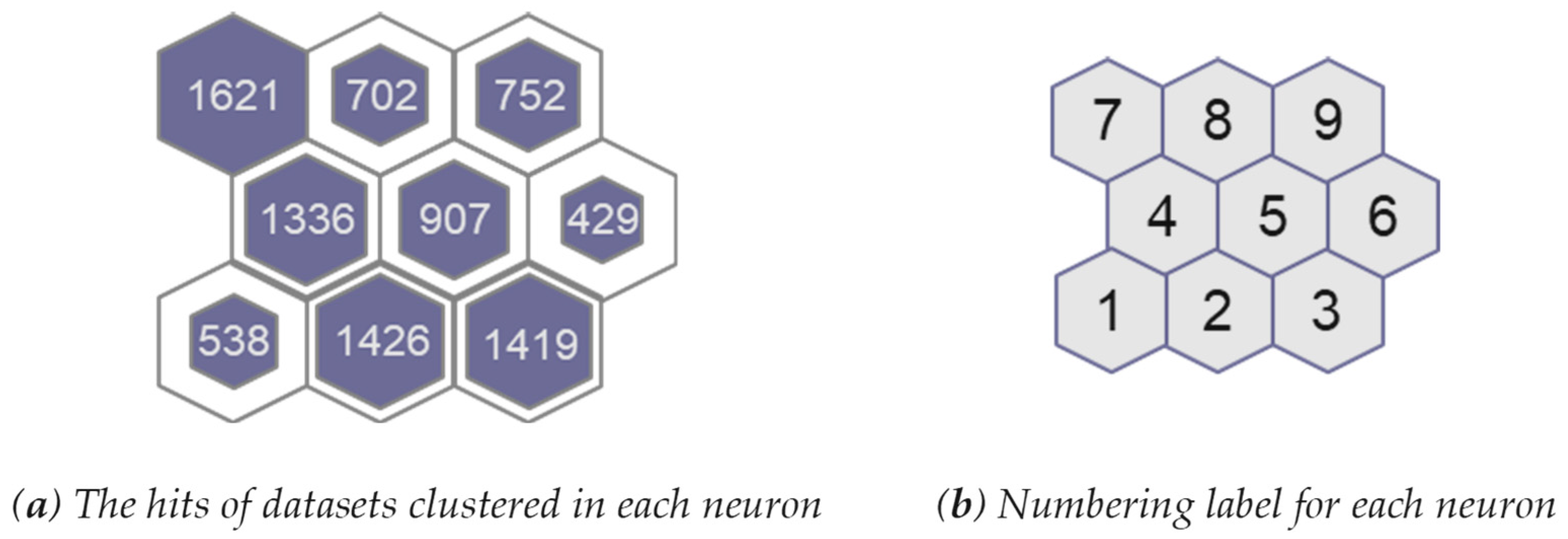
Figure 4.
The heatmap of weather factors and the corresponding characteristics.

Figure 5.
The significance of weather factors in each weather type are transformed into radar diagrams (with examples of weather types #7 and #2). (a) Weather factors integrated into weather type #7. (b) Weather factors integrated into weather type #2.
Figure 5.
The significance of weather factors in each weather type are transformed into radar diagrams (with examples of weather types #7 and #2). (a) Weather factors integrated into weather type #7. (b) Weather factors integrated into weather type #2.

Figure 6.
The occurrence distribution on a 10-day basis for each weather type at Taipei Station.

Figure 7.
The occurrence percentages of the nine weather types at Taipei Station.

Figure 8.
The occurrences distribution of nine weather types on a 10-day basis and the leading types at Taipei Station. (a) Seasonal weather features of sections A, B and C on aggregated occurrences. (b) Leading weather types analysis on a 10-day basis.
Figure 8.
The occurrences distribution of nine weather types on a 10-day basis and the leading types at Taipei Station. (a) Seasonal weather features of sections A, B and C on aggregated occurrences. (b) Leading weather types analysis on a 10-day basis.
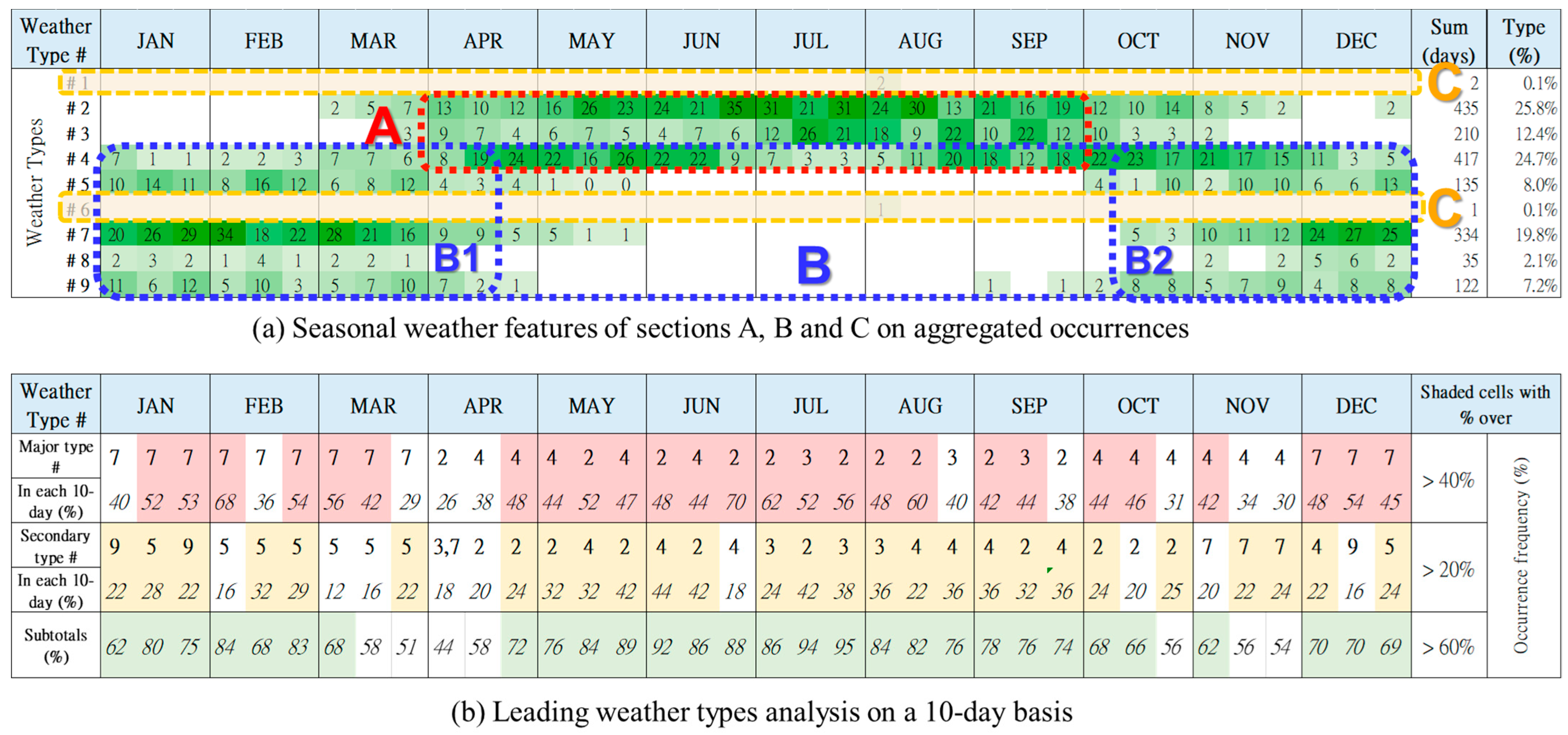
Figure 9.
The occurrence distribution of the main weather types in sections A, B & C at Taipei Station from 2014 and 2018. (a) Section A. (b) Section B & C.
Figure 9.
The occurrence distribution of the main weather types in sections A, B & C at Taipei Station from 2014 and 2018. (a) Section A. (b) Section B & C.
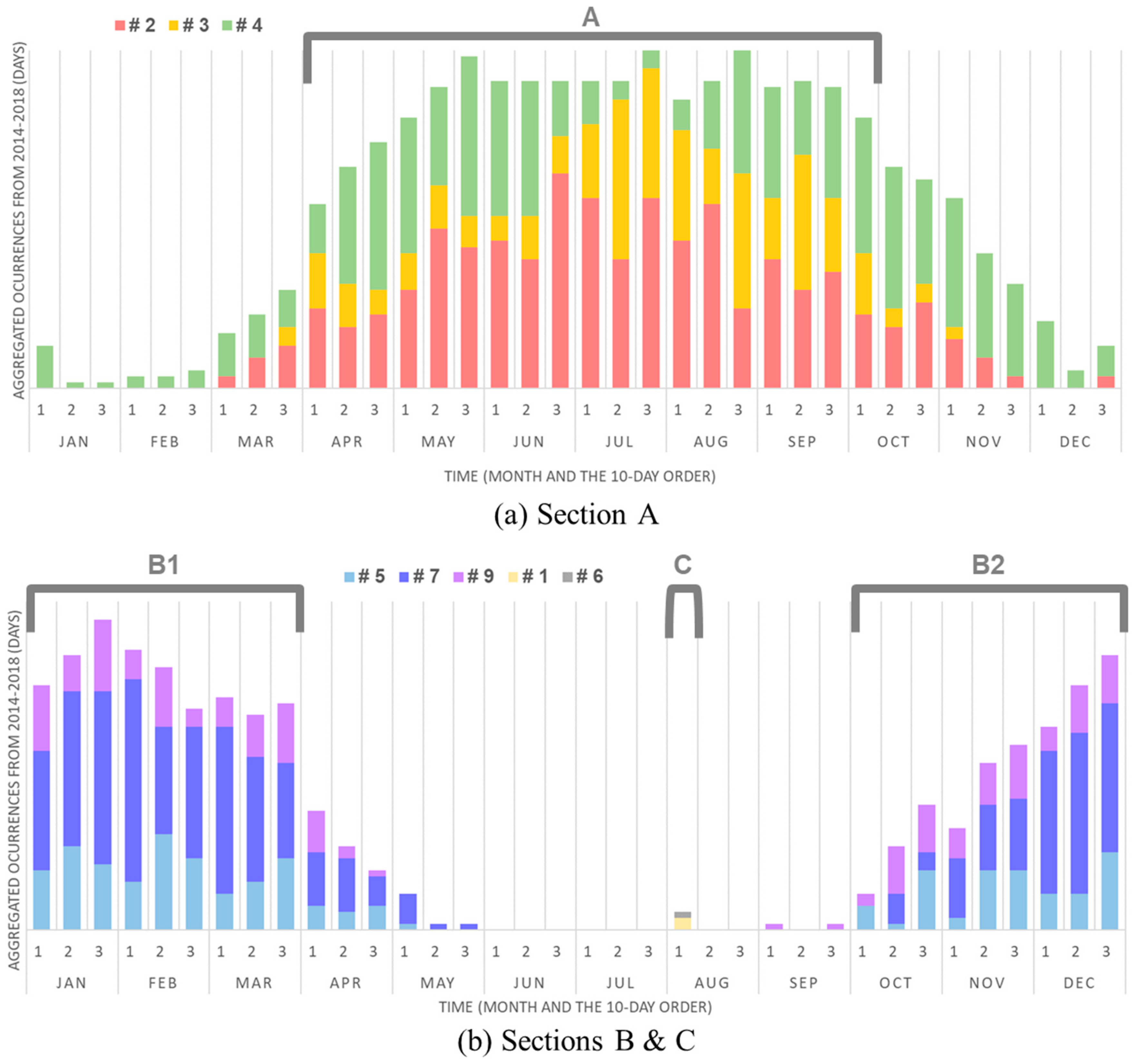
Figure 10.
The leading weather types of Sections A, B, and C in radar diagrams.


Table 1.
Basic statistics of the meteorological data collected at five weather stations in northern Taiwan during 2014–2018.
Table 1.
Basic statistics of the meteorological data collected at five weather stations in northern Taiwan during 2014–2018.
| Station Name | Temperature (°C) | Relative Humidity (%) | Precipitation (mm) | Sunshine Duration (Total h) | Global Radiation (MJ/m2) | Total Cloud Cover (Level 0–10) | |
|---|---|---|---|---|---|---|---|
| Banqiao | Max | 32.3 | 96.0 | 246.0 | 12.7 | 29.8 | 10.0 |
| Min | 5.4 | 46.0 | 0.0 | 0.0 | 0.0 | 0.0 | |
| Avg * | 23.5 | 72.9 | 6.1 | 3.7 | 11.4 | 7.0 | |
| Std ** | 5.5 | 7.9 | 17.0 | 3.5 | 7.3 | 2.6 | |
| Tamshui | Max | 32.3 | 100.0 | 379.5 | 12.5 | 29.1 | 6.7 |
| Min | 5.1 | 1.8 | 0.0 | 0.0 | 0.0 | 0.0 | |
| Avg | 23.0 | 76.7 | 5.4 | 4.5 | 13.2 | 5.0 | |
| Std | 5.5 | 9.4 | 19.7 | 4.0 | 7.8 | 1.6 | |
| Taipei | Max | 33.2 | 97.0 | 306.7 | 11.6 | 28.9 | 10.0 |
| Min | 5.6 | 5.6 | 0.0 | 0.0 | 0.0 | 0.0 | |
| Avg | 23.8 | 23.8 | 6.1 | 3.6 | 12.0 | 7.2 | |
| Std | 5.6 | 5.6 | 18.2 | 3.5 | 7.2 | 2.5 | |
| Xinwu | Max | 31.7 | 100.0 | 246.5 | 12.9 | 30.6 | 10.0 |
| Min | 5.7 | 50.0 | 0.0 | 0.0 | 0.0 | 0.0 | |
| Avg | 23.0 | 79.8 | 3.9 | 5.1 | 14.9 | 6.2 | |
| Std | 5.5 | 8.5 | 14.6 | 4.2 | 8.5 | 2.9 | |
| Keelung | Max | 32.4 | 96.0 | 337.6 | 12.6 | 31.1 | 10.0 |
| Min | 5.4 | 49.0 | 0.0 | 0.0 | 0.0 | 0.0 | |
| Avg | 23.1 | 76.1 | 9.2 | 3.8 | 11.7 | 7.6 | |
| Std | 5.3 | 8.9 | 22.6 | 4.0 | 9.0 | 2.6 | |
| All Stations | Max | 33.2 | 100.0 | 379.5 | 12.9 | 31.1 | 10.0 |
| Min | 5.1 | 1.8 | 0.0 | 0.0 | 0.0 | 0.0 | |
| Avg | 23.3 | 75.6 | 6.1 | 4.2 | 12.6 | 6.6 | |
| Std | 5.5 | 9.1 | 18.7 | 3.9 | 8.1 | 2.7 |
* Average, ** standard deviation.
Table 2.
Features of weather types at 5 weather stations in northern Taiwan.
| Station | Main Types | Occupying Percentage | Absent Types | Summer Types | Concentration in Summer Months | Winter Types | Concentration in Winter Months |
|---|---|---|---|---|---|---|---|
| Banqiao | 4, 7 (1~9) | 40% | 0 | 1, 2, 3, 4, 6 | April–September | 4, 5, 7, 8, 9 | October–March |
| Tamshui | 3, 8 | 55% | 1, 6, 7 | 2, 3, 4 | April–October | 5, 8 | October–May |
| Taipei | 2, 4, 7 | 70% | 1, 6 | 2, 3, 4 | April–October | 5, 7, 8, 9 | October–April |
| Keelung | 1, 5, 6 | 83% | 2, 3, 5 | 4, 6 | April–October | 7, 8 | October–April |
| Xinwu | 2, 3, 4, 7 | 72% | 1, 6 | 2, 3, 4 | April–October | 5, 7, 8, 9 | October–April |
Publisher’s Note: MDPI stays neutral with regard to jurisdictional claims in published maps and institutional affiliations. |
© 2021 by the authors. Licensee MDPI, Basel, Switzerland. This article is an open access article distributed under the terms and conditions of the Creative Commons Attribution (CC BY) license (https://creativecommons.org/licenses/by/4.0/).
Share and Cite
MDPI and ACS Style
Huang, A.; Chang, F.-J. Using a Self-Organizing Map to Explore Local Weather Features for Smart Urban Agriculture in Northern Taiwan. Water 2021, 13, 3457. https://doi.org/10.3390/w13233457
AMA Style
Huang A, Chang F-J. Using a Self-Organizing Map to Explore Local Weather Features for Smart Urban Agriculture in Northern Taiwan. Water. 2021; 13(23):3457. https://doi.org/10.3390/w13233457
Chicago/Turabian StyleHuang, Angela, and Fi-John Chang. 2021. "Using a Self-Organizing Map to Explore Local Weather Features for Smart Urban Agriculture in Northern Taiwan" Water 13, no. 23: 3457. https://doi.org/10.3390/w13233457
Note that from the first issue of 2016, this journal uses article numbers instead of page numbers. See further details here.