
Quantitative Assessment of Uncertainties and Sensitivities in the Estimation of Life Loss Due to the Instantaneous Break of a Hypothetical Dam in Switzerland


Abstract
:1. Introduction
2. Computational Model
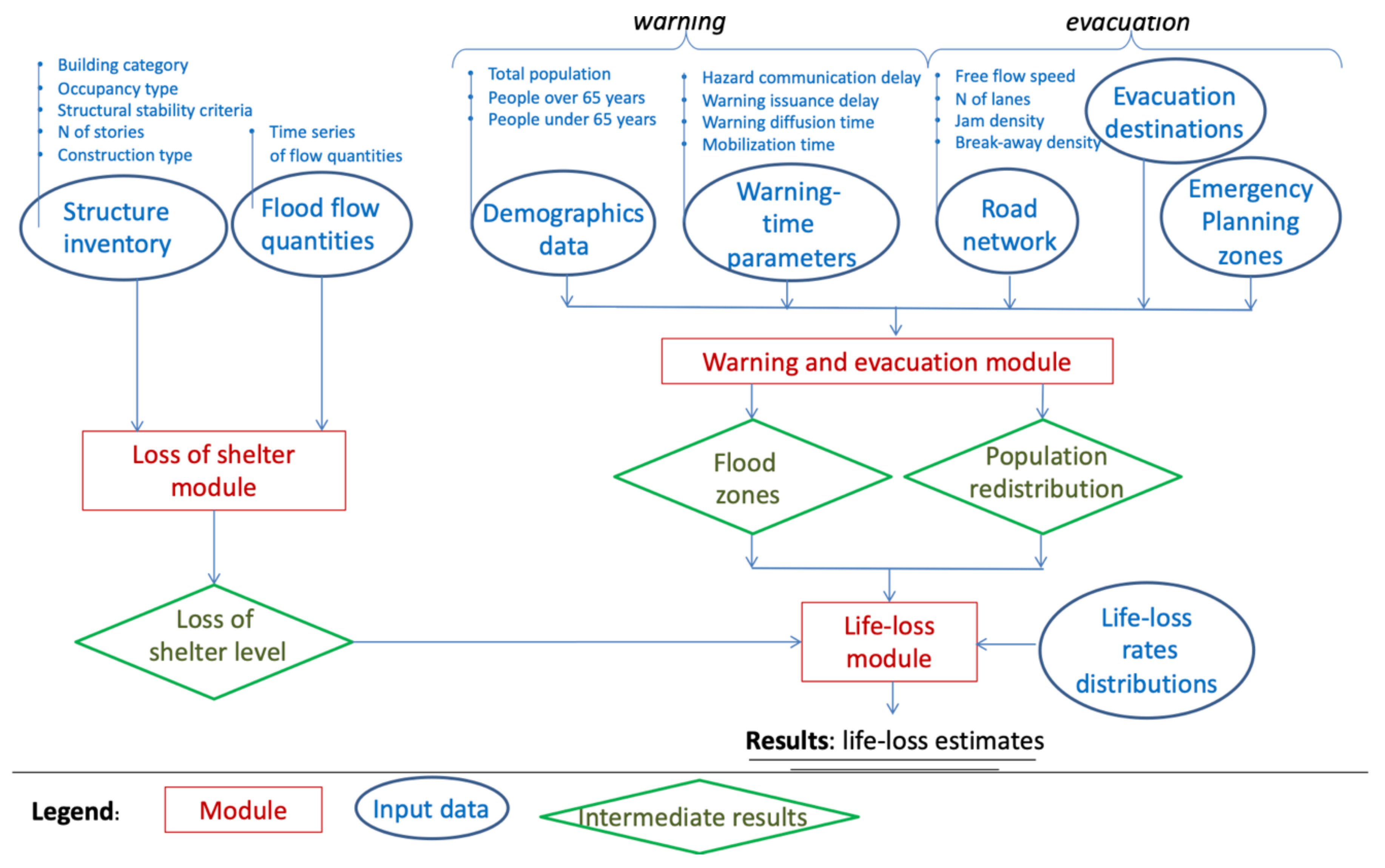
2.1. The HEC-LIFESim Software
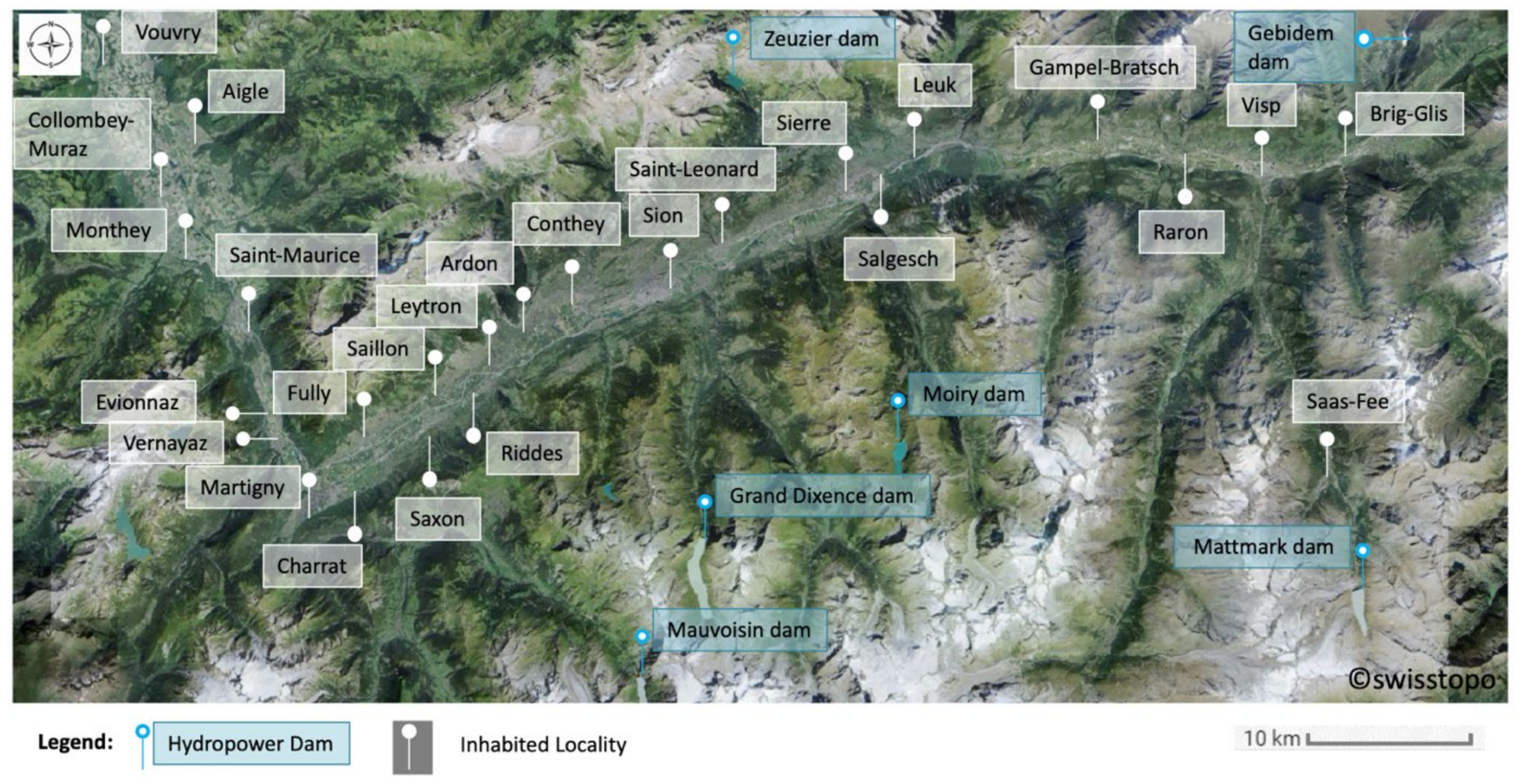
2.2. Information Sources for the Swiss Case Study
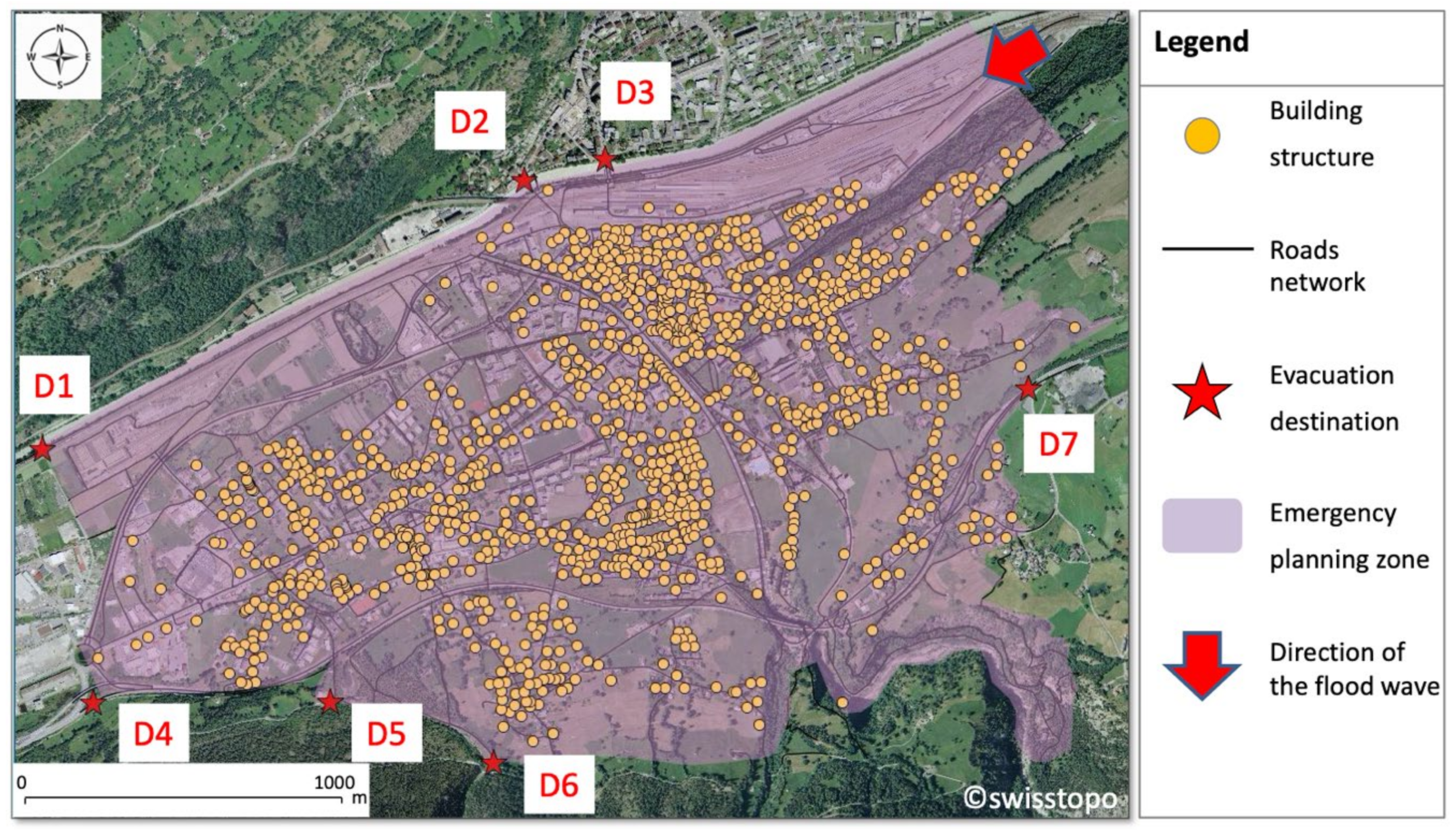
2.2.1. Dam-Downstream Inhabited Locality Representative for Switzerland
- Ratio of building height to building area—0.017 to 0.019 (# floors/m2);
- Total area of its urban part between 1.0 and 3.6 (km2);
- Building density—283.3 to 478.7 (#/m2);
- Fraction of residential among all buildings—92.4 to 96.3 (%).
2.2.2. Swiss Representative Data for the Modules of HEC-LIFESim
Loss of Shelter Module
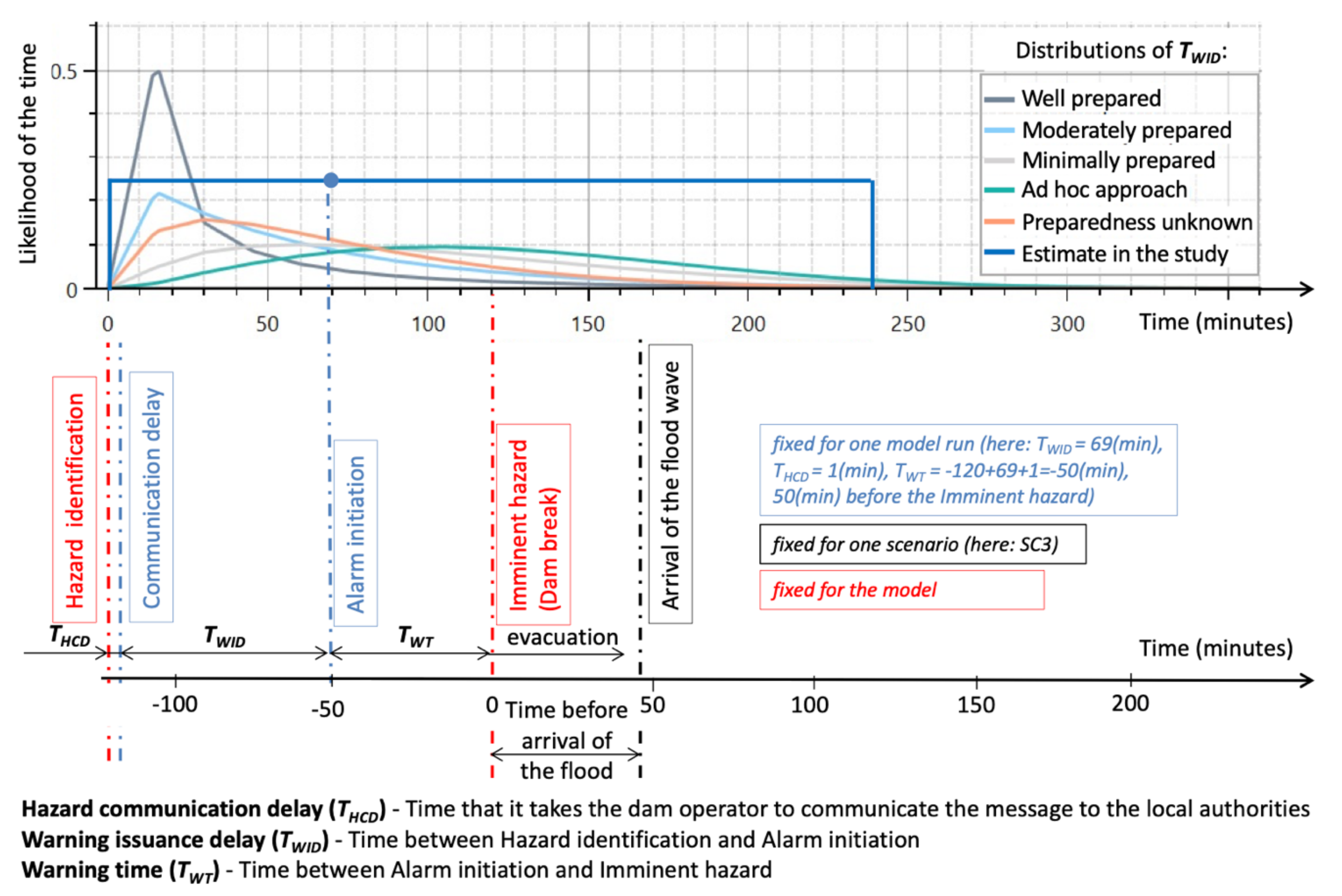
Warning and Evacuation Module
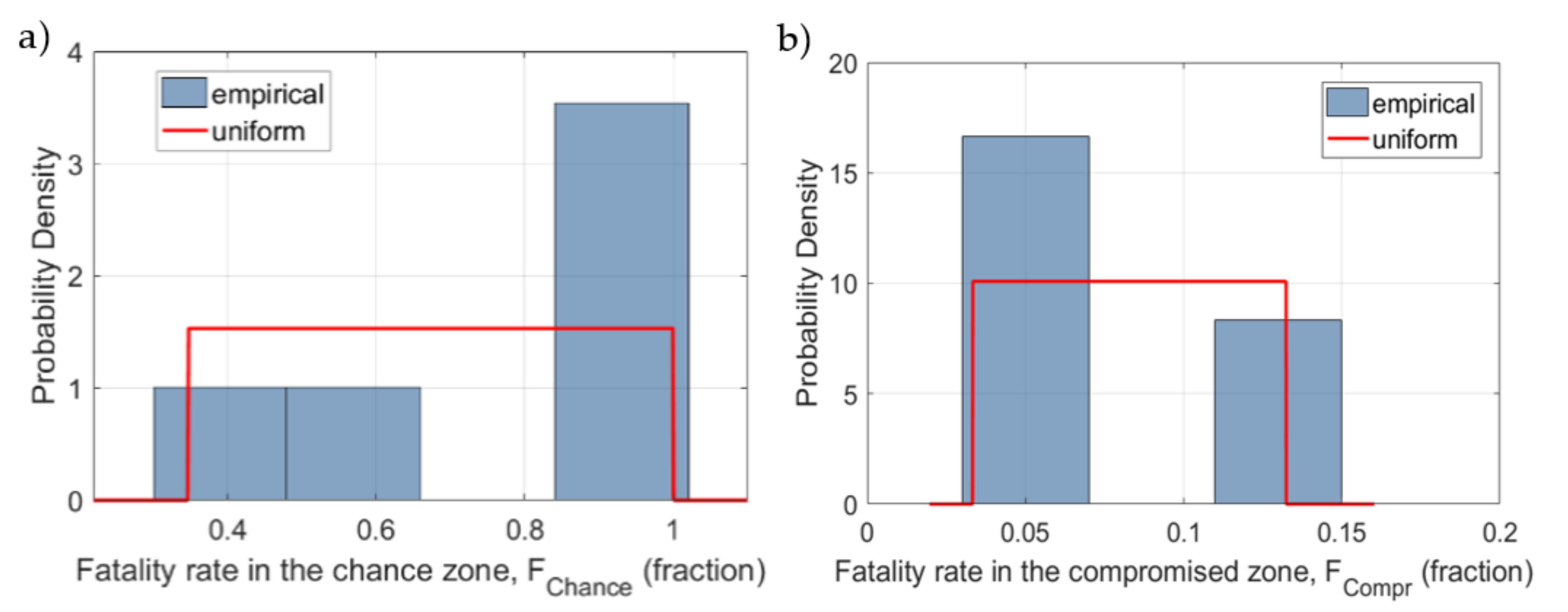
Loss of Life Module
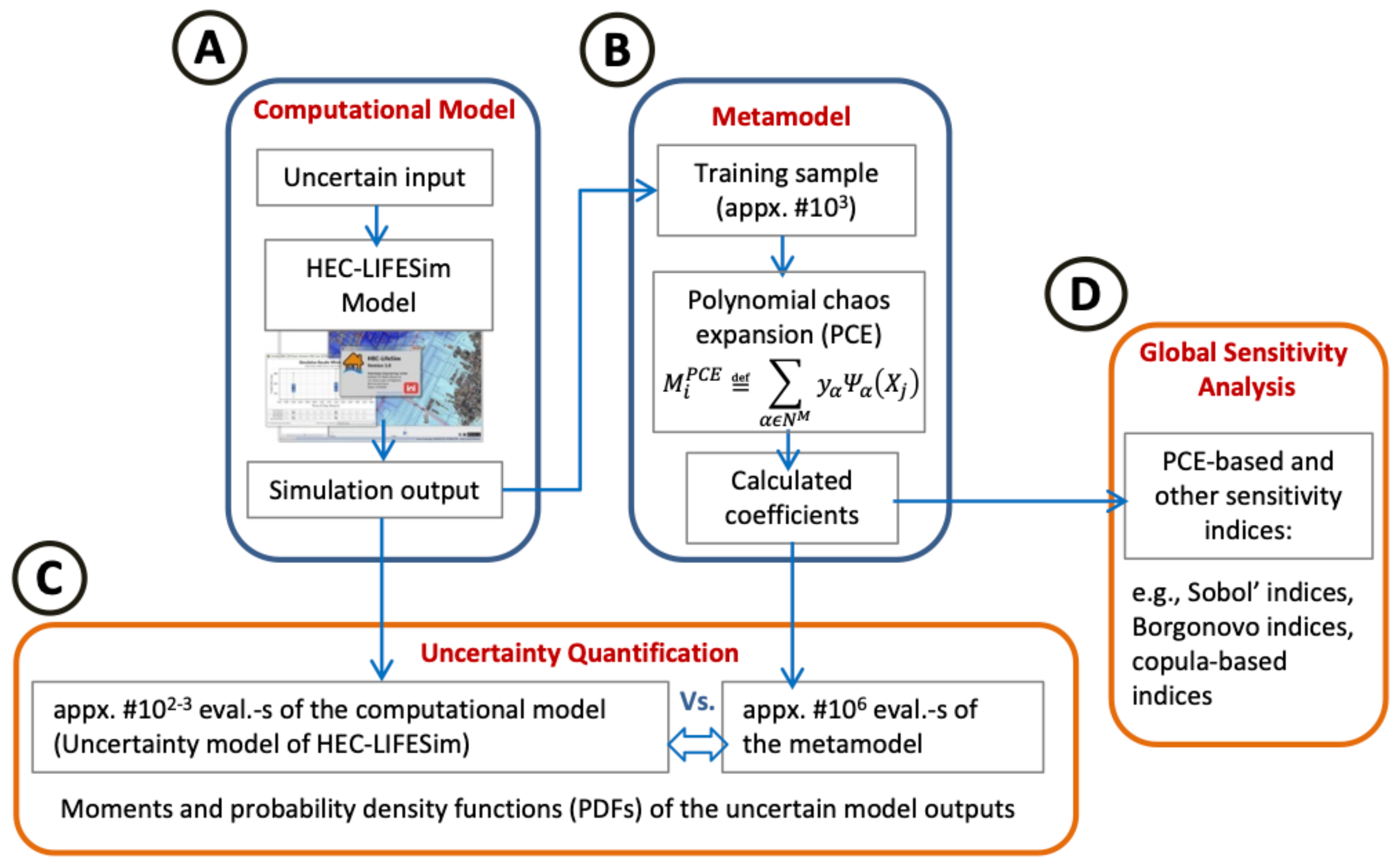
3. Method
3.1. Metamodel
3.1.1. Uncertainty in the Model Input
3.1.2. Uncertainty Propagation
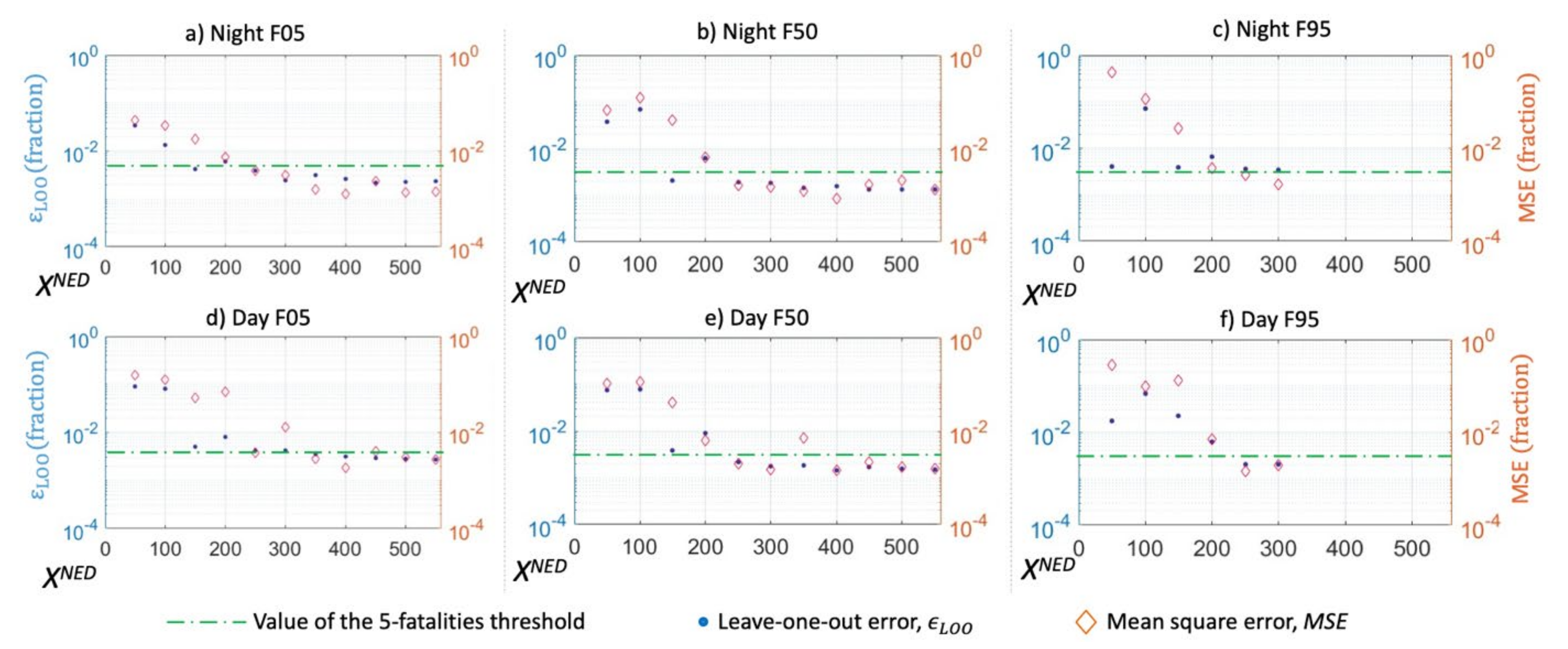
3.1.3. Validation of the Metamodel
3.2. Global Sensitivity Analysis
3.2.1. PCE-Based Sobol’ Indices
3.2.2. Borgonovo Indices
3.3. Definition of the Scenarios
4. Results and Discussion
4.1. Uncertainty in Model Inputs
4.1.1. Definition of the Sources of Uncertainties
4.1.2. Quantification of the Uncertainties in the Input Parameters
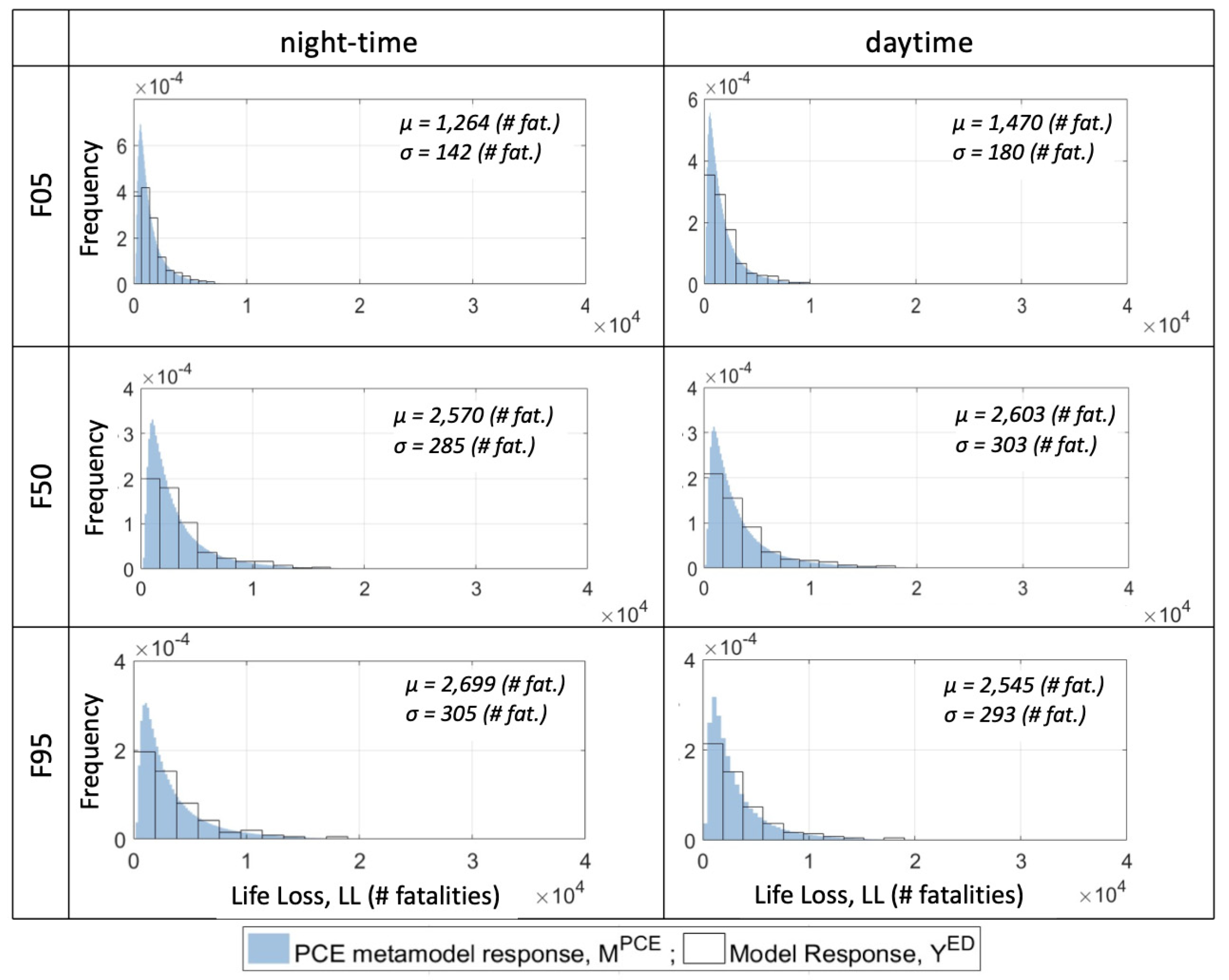
4.2. Uncertainty in Model Output
4.3. PCE and Monte Carlo LL Estimates Comparison
4.4. Global Sensitivity Analysis: Impact of Model Inputs on LL Estimates
5. Conclusions
Supplementary Materials
Author Contributions
Funding
Data Availability Statement
Acknowledgments
Conflicts of Interest
References
- Bureau of Reclamation. Reclamation Consequence Estimating Methodology, RCEM; Guidelines for Estimating Life Loss for Dam Safety Risk Analysis; U.S. Department of the Interior: Washington, DC, USA, 2014. [Google Scholar]
- Darbre, G.R. Dam Risk Analysis; Dam Safety; Federal Office for Water and Geology: Bern, Switzerland, 1999. [Google Scholar]
- Regan, P.E.P.J. An examination of dam failures vs. age of dams. In Proceedings of the 29th Annual USSD Conference, Nashville, TN, USA, 20–24 April 2009. [Google Scholar]
- Bureau of Reclamation. Policy and Procedures for Dam Safety Modification Decisionmaking; Bureau of Reclamation: Denver, CO, USA, 1989; p. 302. [Google Scholar]
- DeKay, M.L.; McClelland, G.H. Predicting loss of life in cases of dam failure and flash flood. Risk Anal. 1993, 13, 193–205. [Google Scholar] [CrossRef]
- Graham, W.J. A Procedure for Estimating Loss of Life Caused by Dam Failure; DSO-99-06; United States Department of the Interior Bureau of Reclamation: Washington, DC, USA, 1999. [Google Scholar]
- McClelland, D.M.; Bowles, D.S. Estimating Life Loss for Dam Safety Risk Assessment—A Review and New Approach; Institute for Dam Safety Risk Management Utah State University: Logan, UT, USA, 2002. [Google Scholar]
- Mao, J.; Wang, S.; Ni, J.; Xi, C.; Wang, J. Management System for Dam-Break Hazard Mapping in a Complex Basin Environment. ISPRS Int. J. Geo Inf. 2017, 6, 162. [Google Scholar] [CrossRef] [Green Version]
- Li, W.; Li, Z.; Ge, W.; Wu, S. Risk Evaluation Model of Life Loss Caused by Dam-break Flood and Its Application. Water 2019, 11, 1359. [Google Scholar] [CrossRef] [Green Version]
- Yudianto, D.; Ginting, B.M.; Sanjaya, S.; Rusli, S.R.; Wicaksono, A. A Framework of Dam-Break Hazard Risk Mapping for a Data-Sparse Region in Indonesia. ISPRS Int. J. Geo Inf. 2021, 10, 110. [Google Scholar] [CrossRef]
- Jonkman, S.N.; Vrijling, J.K. Loss of life due to floods. J. Flood Risk Manag. 2008, 1, 43–56. [Google Scholar] [CrossRef]
- British Columbia, H. Life Safety Model System V1.0, Guidelines, Procedures, Calibration and Support Manual; British Columbia Hydro: Vancouver, BC, USA, 2006. [Google Scholar]
- Lumbroso, D.; Davison, M. Use of an agent-based model and Monte Carlo analysis to estimate the effectiveness of emergency management interventions to reduce loss of life during extreme floods. J. Flood Risk Manag. 2018, 11, S419–S433. [Google Scholar] [CrossRef]
- USACE. HEC-LifeSim. Life Loss Estimation. User’s Manual. Version 1.0; U.S. Army Corps of Engineers, Hydrologic Engineering Center: Davis, CA, USA, 2017. [Google Scholar]
- Bowles, D.S.; Aboelata, M. Evacuation and life-loss estimation model for natural and dam break floods. In Extreme Hydrological Events: New Concepts for Security; Vasiliev, O.F., Ed.; Springer: New York, NY, USA, 2007; Volume 78, pp. 363–383. [Google Scholar]
- Swisstopo. SWISSIMAGE 25 cm. Available online: https://www.swisstopo.admin.ch/en/geodata/images/ortho/swissimage25.html (accessed on 11 January 2019).
- Swisstopo. swissALTI3D. 2018. Available online: https://www.swisstopo.admin.ch/en/geodata/height/alti3d.html (accessed on 11 January 2019).
- Hartford, D.; Baecher, G. Risk and Uncertainty in Dam Safety; Thomas Telford Publishing: London, UK, 2004. [Google Scholar]
- Qi, W.; Zhang, C.; Fu, G.; Sweetapple, C.; Liu, Y. Impact of robustness of hydrological model parameters on flood prediction uncertainty. J. Flood Risk Manag. 2018, 12, e12488. [Google Scholar] [CrossRef] [Green Version]
- Graham, W.J. A comparison of methods for estimating loss of life from dam failure. In Proceedings of the Managing Our Water Retention Systems, 29th Annual USSD Conference, Nashville, TN, USA, 20–24 April 2009. [Google Scholar]
- Lee, J.S. Uncertainties in the Predicted Number of Life Loss due to the Dam Breach Floods. KSCE J. Civ. Eng. 2003, 7, 81–91. [Google Scholar] [CrossRef]
- El Bilali, A.; Taleb, A.; Boutahri, I. Application of HEC-RAS and HEC-LifeSim models for flood risk assessment. J. Appl. Water Eng. Res. 2021, 1–16. [Google Scholar] [CrossRef]
- Aboelata, M.; Bowles, D.S. LIFESim: A tool for estimating and reducing life-loss resulting from dam and levee failures. In Proceedings of the Association of State Dam Safety Officials “Dam Safety 2008” Conference, Indian Wells, CA, USA, 7–11 September 2008. [Google Scholar]
- Aboelata, M.; Bowles, D.S.; McClelland, D.M. A Model for estimating dam failure life loss. In Proceedings of the ANCOLD 2003 Conference on Dams, The Australian Committee on Large Dams Risk Workshop, Launceston, TAS, Australia, October 2003. [Google Scholar]
- Byrne, M.D. How many times should a stochastic model be run? An approach based on confidence intervals. In Proceedings of the 12th International Conference on Cognitive Modeling, Ottawa, ON, Canada, 11–14 July 2013. [Google Scholar]
- Le Gratiet, L.; Marelli, S.; Sudret, B. Metamodel-based sensitivity analysis: Polynomial chaos expansions and gaussian processes. In Handbook of Uncertainty Quantification; Ghanem, R., Higdon, D., Owhadi, H., Eds.; Springer International Publishing: Cham, Switzerland, 2017; pp. 1289–1325. [Google Scholar]
- Sudret, B. Uncertainty Propagation and Sensitivity Analysis in Mechanical Models: Contributions to Structural Reliability and Stochastic Spectral Methods; Habilitation àdiriger des Recherches; Université Blaise Pascal: Clermont-Ferrand, France, 2007. [Google Scholar]
- De Rocquigny, E.; Devictor, N.; Tarantola, S. Uncertainty in Industrial Practice—A Guide to Quantitative Uncertainty Management; John Wiley & Sons: Hoboken, NJ, USA, 2008. [Google Scholar]
- Xiu, D.; Karniadakis, G. The Wiener-Askey polynomial chaos for stochastic equations. SIAM J. Sci. Comput. 2002, 24, 619–644. [Google Scholar] [CrossRef]
- Aboelata, M.A.; Bowles, D.S. LIFESim: A Model for Estimating Dam Failure Life Loss; Report to Institute for Water Resources, US Army Corps of Engineers and Australian National Committee on Large Dams; Institute for Dam Safety Risk Management, Utah State University: Logan, UT, USA, 2005. [Google Scholar]
- Saltelli, A.; Chan, K.; Scott, E.M. Sensitivity Analysis: Wiley Series in Probability and Statistics; John Wiley: Chichester, UK, 2000. [Google Scholar]
- Mokhtari, A.; Frey, H.C. Sensitivity analysis of a two-dimensional probabilistic risk assessment model using analysis of variance. Risk Anal. 2005, 25, 1511–1529. [Google Scholar] [CrossRef]
- Lang, M.; Rehan, B.M.; Hall, J.W.; Klijn, F.; Samuels, P. Uncertainty and sensitivity analysis of flood risk management decisions based on stationary and nonstationary model choices. E3S Web Conf. 2016, 7, 20003. [Google Scholar] [CrossRef] [Green Version]
- Kalinina, A.; Spada, M.; Vetsch, D.; Marelli, S.; Whealton, C.; Burgherr, P.; Sudret, B. Metamodeling for Uncertainty Quantification of a Flood Wave Model for Concrete Dam Breaks. Energies 2020, 13, 3685. [Google Scholar] [CrossRef]
- Saltelli, A.; Ratto, M.; Andres, T.; Campolongo, F.; Cariboni, J.; Galetti, D.; Saisana, M.; Tarantola, S. Global Sensitivity Analysis: The Primer; Wiley: Hoboken, NJ, USA, 2008. [Google Scholar]
- Delenne, C.; Cappelaere, B.; Guinot, V. Uncertainty analysis of river flooding and dam failure risks using local sensitivity computations. Reliab. Eng. Syst. Saf. 2012, 107, 171–183. [Google Scholar] [CrossRef] [Green Version]
- Sobol, I.M. Global sensitivity indices for nonlinear mathematical models and their Monte Carlo estimates. Math. Comput. Simul. 2001, 55, 271–280. [Google Scholar] [CrossRef]
- Frey, H.C.; Patil, S.R. Identification and review of sensitivity analysis methods. Risk Anal. 2002, 22, 553–578. [Google Scholar] [CrossRef]
- Tene, M.; Stuparu, D.E.; Kurowicka, D.; El Serafy, G.Y. A copula-based sensitivity analysis method and its application to a North Sea sediment transport model. Environ. Model. Softw. 2018, 104, 1–12. [Google Scholar] [CrossRef] [Green Version]
- Borgonovo, E. A new uncertainty importance measure. Reliab. Eng. Syst. Saf. 2007, 92, 771–784. [Google Scholar] [CrossRef]
- Iooss, B.; Lemaître, P. A review on global sensitivity analysis methods. In Uncertainty Management in Simulation-Optimization of Complex Systems: Algorithms and Applications; Dellino, G., Meloni, C., Eds.; Springer US: Boston, MA, USA, 2015; pp. 101–122. [Google Scholar]
- Zhang, L.; Peng, M.; Chang, D.; Xu, Y. Dam Failure Mechanisms and Risk Assessment, 1st ed.; Jon Wiley & Sons Singapore Pte. Ltd.: Singapore, 2016. [Google Scholar]
- ESRI. ESRI Products, Software, and Services; Environmental Systems Research Institute: Redlands, CA, USA, 2017. [Google Scholar]
- Bowles, D.S. Life loss estimation for RAMCAP, Appendix D. In Conventional Dams and Navigation Locks, Sector-Specific Guidance (SSG), Risk Analysis and Management for Critical Asset Protection (RAMCAP) Phase III for Dams, Locks and Levees; CISA: Arlington, VA, USA, 2007. [Google Scholar]
- McClelland, D.M.; Bowles, D. Estimating life loss for dam safety and risk assessment: Lessons from case histories. In Proceedings of the 2000 Annual USCOLD Conference, U.S. Society on Dams, Denver, CO, USA, 5–8 August 2000. [Google Scholar]
- Branch, M.C. Common characteristics of new towns. Cities 1983, 1, 146–149. [Google Scholar] [CrossRef]
- Chen, Y.J.; Matsuoka, R.H.; Liang, T.M. Urban form, building characteristics, and residential electricity consumption: A case study in Tainan City. Environ. Plan. B Urban Anal. City Sci. 2017, 45, 933–952. [Google Scholar] [CrossRef]
- SFSO. Regionalporträts 2017: Kennzahlen aller Gemeinden; je-d-21.03.01; Swiss Federal Statistical Office: Bern, Switzerland, 2017. [Google Scholar]
- SFSO. Eidgenössisches Gebäude- und Wohnungsregister. Version 3.7.; The Federal Department of Home Affairs: Neuchâtel, Switzerland, 2018. [Google Scholar]
- FEI. Development of Rescue Actions Based on Dam-Break Flood Analysis, RESCDAM; Finnish Environmental Insititute: Helsinki, Finland, 2001. [Google Scholar]
- World Bank. Doing Business 2019. Training for Reform; World Bank: Washington, DC, USA, 2019. [Google Scholar]
- USACE. HEC-RAS 5.0.3; U.S. Army Corps of Engineers, Hydrologic Engineering Center: Davis, CA, USA, 2017. [Google Scholar]
- SFSO. Ständige und Nichtständige Wohnbevölkerung Nach Institutionellen Gliederungen, Geburtsort und Staatsangehörigkeit; (STAT-TAB); Swiss Federal Statistical Office: Bern, Switzerland, 2017. (In German) [Google Scholar]
- WRFA. Water Retaining Facilities Act; WRFA: Jamestown, NY, USA, 2013. [Google Scholar]
- SFOE. Directive on the Safety of Water Retaining Facilities, Part D: Commissioning and Operation; Swiss Federal Office of Energy: Bern, Switzerland, 2015. [Google Scholar]
- Public Safety Department of the Municipality of Brig-Glis. Notfallinfo. Available online: https://www.brig-glis.ch/sicherheit/ (accessed on 8 October 2018).
- OpenStreetMap. Open Data Commons Open Database License. 2018. Available online: https://opendatacommons.org/licenses/odbl/ (accessed on 8 October 2018).
- Kalinina, A.; Spada, M.; Burgherr, P. Alternative life-loss rates for failures of large concrete and masonry dams in mountain regions of OECD countries. In Proceedings of the Safety and Reliability of Complex Engineered Systems: ESREL, Trondheim, Norway, 17–21 June 2018. [Google Scholar]
- Zellnerr, A.; Highfiled, R. Calculation of Maximum Entropy Distributions and Approximation of Marginal Posterior Distributions. J. Econom. 1988, 37, 195–209. [Google Scholar] [CrossRef]
- Lingam, M.; Comisso, L. A maximum entropy principle for inferring the distribution of 3D plasmoids. Phys. Plasmas 2018, 25, 012114. [Google Scholar] [CrossRef] [Green Version]
- De Martino, A.; De Martino, D. An introduction to the maximum entropy approach and its application to inference problems in biology. Heliyon 2018, 4, e00596. [Google Scholar] [CrossRef] [PubMed] [Green Version]
- Bhat, H.S.; Kumar, N. On the Derivation of the Bayesian Information Criterion; School of Natural Sciences, University of California: Oakland, CA, USA, 2010. [Google Scholar]
- Akaike, H. A new look at the statistical model identification. IEEE Trans. Autom. Control 1974, 19, 716–723. [Google Scholar] [CrossRef]
- Limpert, E.; Stahel, W.A.; Abbt, M. Log-normal Distributions across the Sciences: Keys and Clues. BioScience 2001, 51, 341–352. [Google Scholar] [CrossRef]
- Matz, A.W. Maximum Likelihood Parameter Estimation for the Quartic Exponential Distribution. Technometrics 1978, 20, 475–484. [Google Scholar] [CrossRef]
- Ghanem, R.; Spanos, P. Stochastic Finite Elements—A Spectral Approach; Springer: New York, NY, USA, 1991. [Google Scholar]
- McKay, M.D.; Beckman, R.J.; Conover, W.J. A comparison of three methods for selecting values of input variables in the analysis of output from a computer code. Technometrics 1979, 2, 239–245. [Google Scholar]
- Efron, B.; Hastie, T.; Johnstone, I.; Tibshirani, R. Least angle regression. Ann. Stat. 2004, 32, 407–499. [Google Scholar] [CrossRef] [Green Version]
- Marelli, S.; Sudret, B. UQLab: A framework for uncertainty quantification in Matlab 257 Vulnerability, Uncertainty, and Risk. In Proceedings of the 2nd International Conference on Vulnerability, Risk Analysis and Management (ICVRAM2014), Liverpool, UK, 13–16 July 2014; pp. 2554–2563. [Google Scholar]
- Marelli, S.; Sudret, B. UQLab User Manual—Polynomial Chaos Expansions; Technical Report; Chair of Risk, Safety & Uncertainty Quantification, ETH: Zürich, Switzerland, 2017. [Google Scholar]
- Blatman, G.; Sudret, B. Adaptive sparse polynomial chaos expansion based on Least Angle Regression. J. Comput. Phys. 2011, 230, 2345–2367. [Google Scholar] [CrossRef]
- Blatman, G.; Sudret, B. An adaptive algorithm to build up sparse polynomial chaos expansions for stochastic finite element analysis. Probabilistic Eng. Mech. 2010, 25, 183–197. [Google Scholar] [CrossRef]
- Marelli, S.; Lamas, C.; Sudret, B.; Konakli, K.; Mylonas, C. UQLab User Manual—Sensitivity Analysis; Chair of Risk, Safety & Uncertainty Quantification, ETH: Zürich, Switzerland, 2018. [Google Scholar]
- Brevault, L.; Balesdent, M.; Berend, N.; Le Riche, R. Comparison of different global sensitivity analysis methods for aerospace vehicle optimal design. In Proceedings of the 10th World Congress on Structural and Multidisciplinary Optimization, Orlando FL, USA, 19–24 May 2013. [Google Scholar]
- Zhang, X.-Y.; Trame, M.N.; Lesko, L.J.; Schmidt, S. Sobol Sensitivity Analysis: A Tool to Guide the Development and Evaluation of systems Pharmacology Models. CPT Pharmacomet. Syst. Pharmacol. 2015, 4, 69–79. [Google Scholar] [CrossRef]
- Sobol, I. Sensitivity estimates for nonlinear mathematical models. Math. Comput. Model. 1993, 1, 407–414. [Google Scholar]
- Sudret, B. Global sensitivity analysis using polynomial chaos expansions. Reliab. Eng. Syst. Saf. 2008, 93, 964–979. [Google Scholar] [CrossRef]
- Baecher, G.B. Uncertainty in dam safety risk analysis. GEORISK 2016, 10, 92–108. [Google Scholar] [CrossRef]
- Graham, W.J. A Procedure for Estimating Loss of Life Caused by Dam Failure; Sedimentation & River Hydraulics: Denver, CO, USA, 1999. [Google Scholar]
- Wang, C.; Zhand, S.; Tan, Y.; Pan, F.; Yan, L. Life Loss Estimation Based on Dam-Break Flood Uncertainties and Lack of Information in Mountainous Regions of Western China. Trans. Tianjin Univ. 2017, 23, 370–379. [Google Scholar] [CrossRef]
- Hirschberg, S.; Spiekerman, G.; Dones, R. Severe Accidents in the Energy Sector, 1st ed.; PSI Report 98-16; Paul Scherrer Institut: Villigen PSI, Switzerland, 1998. [Google Scholar]
- Darbre, G.R. Dam breach in the context of dam safety legislation. In Proceedings of the SwissCOD/VAW Workshop on Dam Breach Analysis, Bern, Switzerland, 26 April 2017. [Google Scholar]
- SFOE. Methodik zur Bestimmung der Anzahl Gefährdeter Personen (People at Risk PAR) zur Abschätzung der Hohen Gefahr (Version 1.0); Swiss Federal Office of Energy, Sektion Aufsicht Talsperren: Bern, Switzerland, 2017. (In German) [Google Scholar]


| F05 | F50 | F95 | ||
|---|---|---|---|---|
 | ||||
| (m3/s) | 6.57 × 10³ | 6.25 × 10⁴ | 3.17 × 10⁵ | |
| (s) | 129.72 | 522.05 | 3.93 × 10³ | |
| (s) | 31.55 | 340.10 | 2.84 × 10³ | |
| (m3/s2) | 4.60 × 10⁻⁴ | 0.0011 | 0.0024 | |
| Parameter | Name | Unit | Definition |
|---|---|---|---|
| Receptor | |||
| Total population | # people | Total population of the modelled inhabited locality | |
| Population over 65 | fraction | Part of the total population older than 65 years | |
| H | Building foundation height | m | Height between the level of the ground and the level of the ground floor in the building |
| Reaction | |||
| Fatality rate in the chance zone | fraction | Fatality rate in the chance zone given as a part of PAR that will lose their life | |
| Fatality rate in the compromised zone | fraction | Fatality rate in the compromised zone given as a part of PAR that will lose their life | |
| Hazard communication delay | h | Time that it takes the dam operator to communicate the message to the local authorities | |
| Warning issuance delay | h | Time that it takes the local authorities to initiate warning | |
| Author (Year) | Paper Title | Warning Time (h) |
|---|---|---|
| DeKay and McClelland [5] | Predicting loss of life in cases of dam failure and flash flood | from −4 * to 0 |
| Graham [79] | A Procedure for Estimating Loss of Life Caused by Dam Failure | from −1 to 0 |
| Darbre [2] | Dam Risk Analysis | from 0.25 to 0.5 |
| Bowles and Aboelata [12] | Evacuation and life-loss estimation model for natural and dam break floods | from −3 to 2 |
| Wang et al. [80] | Life Loss Estimation Based on Dam-Break Flood Uncertainties and Lack of Information in Mountainous Regions of Western China | from −2 to 0 |
| Parameter | Unit | Distribution | Hyper-Parameters | Truncation | Mean and Variance |
|---|---|---|---|---|---|
| Receptor | |||||
| # people | [1400 34,000] | 7.35 × 10³, 8.21 × 10³ | |||
| fraction | - | 0.17, 0.027 | |||
| m | - | 0.85, 0.38 | |||
| Reaction | |||||
| fraction | - | 0.67, 0.19 | |||
| fraction | - | 0.083, 0.029 | |||
| h | - | 2, 1.15 | |||
| h | - | 0.13, 0.072 | |||
Publisher’s Note: MDPI stays neutral with regard to jurisdictional claims in published maps and institutional affiliations. |
© 2021 by the authors. Licensee MDPI, Basel, Switzerland. This article is an open access article distributed under the terms and conditions of the Creative Commons Attribution (CC BY) license (https://creativecommons.org/licenses/by/4.0/).
Share and Cite
Kalinina, A.; Spada, M.; Burgherr, P. Quantitative Assessment of Uncertainties and Sensitivities in the Estimation of Life Loss Due to the Instantaneous Break of a Hypothetical Dam in Switzerland. Water 2021, 13, 3414. https://doi.org/10.3390/w13233414
Kalinina A, Spada M, Burgherr P. Quantitative Assessment of Uncertainties and Sensitivities in the Estimation of Life Loss Due to the Instantaneous Break of a Hypothetical Dam in Switzerland. Water. 2021; 13(23):3414. https://doi.org/10.3390/w13233414
Chicago/Turabian StyleKalinina, Anna, Matteo Spada, and Peter Burgherr. 2021. "Quantitative Assessment of Uncertainties and Sensitivities in the Estimation of Life Loss Due to the Instantaneous Break of a Hypothetical Dam in Switzerland" Water 13, no. 23: 3414. https://doi.org/10.3390/w13233414
APA StyleKalinina, A., Spada, M., & Burgherr, P. (2021). Quantitative Assessment of Uncertainties and Sensitivities in the Estimation of Life Loss Due to the Instantaneous Break of a Hypothetical Dam in Switzerland. Water, 13(23), 3414. https://doi.org/10.3390/w13233414