1. Introduction
According to projections, climate change will reduce both surface and groundwater resources leading to rapid increases in water scarcity [
1,
2,
3]. In this context, urban areas may be particularly affected and will face increased risks from rising temperatures, extreme storms and precipitation, water scarcity, droughts and floods [
4].
The size and growth of the urban population and the increasing complexity of providing all the necessary services to this population make cities highly vulnerable to the effects of climate change [
5,
6,
7]. According to OECD [
8], in order to tackle water problems, it is urgent that city governments and municipalities promote more effective and sustainable urban water management. However, urban water demand management policies that are effective in reducing consumption require an in-depth understanding of consumer behaviour.
In this context, the aim of this paper is to analyse domestic water demand by trying to capture unobserved heterogeneity using a hierarchical model at an intra-urban scale. The complexity of residential water demand can be clearly seen in the different results obtained in the literature depending on the local characteristics, the variables incorporated in the analysis, the functional form employed, the data aggregation level and the methodologies used [
9,
10,
11,
12,
13].
The literature recognises that studies that have used microdata in their analyses [
14,
15,
16,
17,
18,
19,
20,
21,
22,
23] are better able to capture differences in water consumption between individuals [
9,
11]. However, only a few studies have exploited household-level databases in their estimates (36% of the sample used by Marzano et al. [
12]).
According to Flores-Arévalo et al. [
23], databases that present all information at the household level are an exception in the literature. Similarly, panel data are also preferred when capturing household heterogeneity over time [
23]. Thus, panel data that present all variables disaggregated at the household level are preferred but rarely present in the literature [
24,
25,
26].
Two methodological perspectives were adopted to address the high variability in the behaviour of domestic water consumption between individuals or unobserved heterogeneity and between spatial or temporal scales. Research on unobservable heterogeneity and to address the problems of scale in urban water demand has been considered of great interest in the literature. House-Peters and Chang [
27] presented a review of methodological developments in urban water demand modelling incorporating scale analysis. They recognised that variations in consumption at the neighbourhood or census block scale are important determinants of water demand.
A first approach that attempted to capture the influence of the local environment on the water consumption in cities incorporated variables related to geography and demography into studies of water demand, which made it possible to relate consumption to urban structure [
28,
29,
30,
31,
32,
33,
34,
35].
Another approach that has made it possible to study the variability of consumption in relation to consumer’s location context is the introduction of different spatial scales, understood as a unit of analysis. This approach includes studies that analysed several cities with household data [
36,
37]. Other research have used intra-city scale data (with data from some administrative division of cities) in their analysis with the aim of capturing different behaviours within the city (examples of these are the studies for United States [
32,
38,
39,
40,
41,
42] and for Australia [
43]).
Finally, some research has used several scales of analysis in their studies. Ouyang et al. [
44] analysed the domestic water demand in the Phoenix metropolitan area using three analysis scales (household, district and city), estimating a different demand function for each scale.
The problem of unobservable heterogeneity has also received some attention in the literature with papers whose main objective has been to introduce individual heterogeneity into their analyses. Attempts were made to control for that problem using a variety of methodological approaches: the inclusion of fixed effects at the household level [
45]; the estimation of models comparing fixed and random effects [
46]; the random coefficients model [
47]; estimation of demand by group [
37,
48]; and the latent class model (LCM), dividing consumers into homogeneous groups without the need for a priori selection to estimate the demand [
49], quantile regression [
50] and instrumental variables regression approach [
51].
In many of the papers that attempted to address the problem of unobserved individual heterogeneity with their models, the authors concluded that there are differences between the groups of consumers that they consider [
37,
47,
48]. In the study by Pérez-Urdiales and García-Valinas [
49], a range of elasticities of −1.23 to 0.9 was found. In the study by Wichman [
52], the range was −1.43 to −1.14.
The model used in this paper is a hierarchical model (also known as multilevel or mixed model analysis). Given that the available data (a large panel with disaggregated data at household level) have a multilevel structure, multilevel analysis can be used to study water demand to capture the heterogeneity in domestic consumption. Thus, the methodology consisted of estimating a demand function through a mixed model that included the intraurban scale in the analysis and enabled in-depth analysis of the differences in consumption between different individuals from different neighbourhoods in different periods.
Few studies in the literature on domestic water demand have used hierarchical models in their analysis. The introduction of the spatial scale in studies of domestic demand in cities is not common, and there are no studies of this type for Spanish cities. This application of a suburban multilevel model is very limited elsewhere. In this sense, main contribution of this paper is the analysis of unobserved heterogeneity using a hierarchical model.
Therefore, with the application of a mixed effects analysis, which allows for the incorporation of temporal and spatial scale effects in a hierarchical or multilevel manner, the analysis aimed at capturing heterogeneity within the city building on earlier analysis using panel techniques and the introduction of a fixed effect for each neighbourhood [
53].
This article has five sections. Following this Introduction,
Section 2 describes the study area, the conurban area of the city of Valencia.
Section 3 focuses on the database used in the estimates of domestic water demand, the methodological approach and the estimated model.
Section 4 presents the results.
Section 5 offers the discussion and general conclusions derived from the results as well as future lines of research.
2. Study Area Description
The empirical analysis of domestic water demand in the city of Valencia is motivated by several characteristics of this urban area, which is the third largest in Spain, behind Madrid and Barcelona. The city of Valencia represents 51.2% of the total population of the conurban area, and its population density is around 8000 inhabitants per square kilometre. Although, in general terms, there has been large population growth in the city since the 1960s, in the period under analysis, between 2009 and 2011, there was a decline. From 2015, there was a change in trend that has persisted to the present day.
The total surface area of the city of Valencia is 13,748 hectares, with much of this area occupied by crops and wetlands. Most of these crop and wetland areas are located to the south of the city and correspond to the area surrounding the Albufera lake. In 1986, the system formed by the lake, its wetlands and the coastal bar adjacent to both (a total area of 21,120 hectares) was declared a natural park. The natural park includes meadow areas, market garden crops and rice crops in the wetland area of marshes surrounding the Albufera. Thus, the highly protected status of the natural park, its proximity to the city of Valencia and, above all, the wetland area put major pressure on the use of water resources.
Another source of pressure on resources is related to the economic activity of Valencia, which is fundamentally centred on services. These service activities are strongly related to the evolution of the tourism sector, which represents a large and growing part of the activity of the city. More than 65% of the economic activity in Valencia corresponds to commerce and services. Although tourism activity in the case of Valencia does not, in general, have a direct impact on domestic water consumption, it does put additional pressure on the available resources [
54,
55,
56].
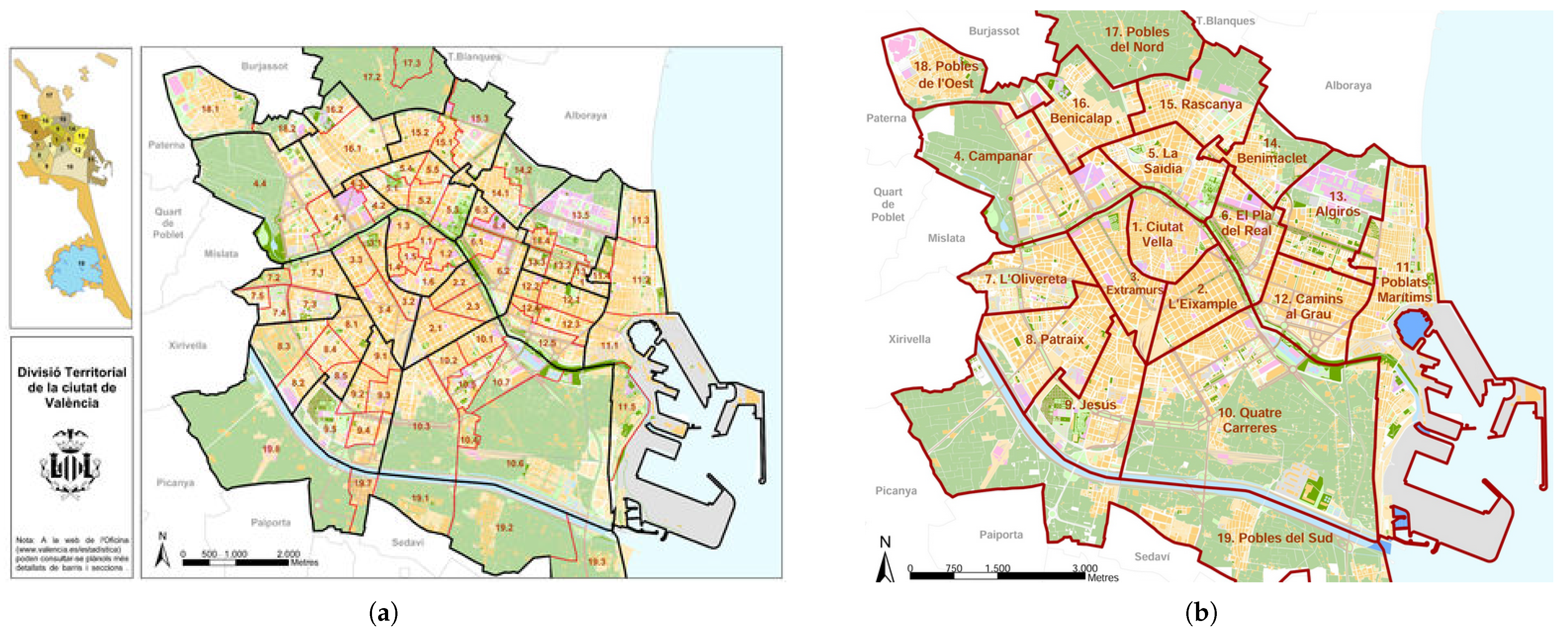
With regard to the administrative division of Valencia, the city is divided into 19 administrative districts and 87 administrative neighbourhoods (see
Figure 1). There are major socioeconomic differences between them, which may have an impact on the behaviour of drinking water consumers. Nonetheless, the most relevant feature of the city of Valencia is the domestic water pricing. The tariff structure, which is based on an increasing rate tariff (IRT), differs from those typically used for domestic consumption. In addition, a charge is added for the metropolitan urban waste treatment and disposal service (TAMER charge), with a fixed or fixed-plus-variable charge (depending on the previous year’s consumption). In any case, the TAMER charge increases the proportion of the fixed part of the price of the bill.
According to data from the statistical yearbooks of the city of Valencia (2008–2011) [
57], among districts and neighbourhoods, there are large differences in income level, land use and degree of urbanisation. Income levels in the different districts are in the range of 70% above and below the city average. Land use and degree of urbanisation are reflected by population density data, with districts that have up to three times the population density of the city average and peripheral districts with a much lower degree of urbanisation and a population density below the average. Whereas some areas are highly urbanised, others have a high proportion of undeveloped land.
These differences are more pronounced when analysing the data at a higher level of disaggregation. While none of the districts exceeded 30,000 inhabitants per km2 in 2011, at the neighbourhood level, 23 of them exceeded this figure.The reason is a process of urban growth in the south and west of the city, which has increased the density of certain neighbourhoods. In addition, the surface area of the northern and southern peripheral districts (which include part of the Albufera nature reserve) is mainly dedicated to crops (either rice production or market gardens), which explains the low population density in all of these neighbourhoods.
Differences in income and population density between districts and neighbourhoods may influence the behaviour of drinking water consumers. Indeed, the data on domestic water consumption reveal significant differences at intra-urban level. Thus, while the average consumption at city level in 2011 was 152.3 L per person per day, eleven of the eighteen districts had consumption above the average, and four of them consumed more than 200 L per person per day. The temporal evolution of consumption in certain districts was not the same as the city average, since some districts increased their average consumption in the period 2008 to 2011, while others decreased it.
In general terms, the average water consumption in the city of Valencia and its evolution in the period of analysis was heterogeneous with neighbourhoods where consumption did not vary significantly and remained in the high or low ranges. Nonetheless, as stated above, a relevant feature of the city of Valencia is the domestic water pricing. Unlike most cities that apply the IBT tariffs [
58,
59,
60,
61], in the city of Valencia, the tariff structure is based on an increasing rate tariff (IRT) [also known as increasing average price tariffs (IAPT)], where the variable charge is obtained by multiplying household consumption by a price that varies depending on consumption [
58].
The water bill in the city of Valencia includes all payments that a consumer makes for the services within the urban water cycle, including payments for supply, sewerage and sanitation. More specifically, the water bill includes the prices or tariffs for water supply (low and upstream), payments for the sewerage services phase, the City Council’s investment fees and the fees of the Jucar Basin Authority (CHJ). In addition, a charge is added for the metropolitan urban waste treatment and disposal service (TAMER charge). Each payment has a different structure and legal nature.
The low water supply tariffs have a two-part IRT structure: a fixed part that depends on the size of the meter and a variable part in two blocks with a limit of 12 m3 bimonthly for the first block. The upstream water supply tariff has a one-part structure (not including fixed charges) that corresponds to a uniform volume-based payment. In the payments for sewerage services, there is a sewerage charge with a uniform variable price in addition to a sanitation charge. The latter charge also has a two-part structure.
The variable part is uniform and is the same for all m3 consumed. Both the variable and the fixed parts of the charge depend on the size of the municipality. In the case of Valencia, the size corresponds to the section with more than 50,000 inhabitants. To these payments are added the City Council’s investment fee (which is established as a fixed amount per month (€/month)) and the Jucar Hydrographic Confederation fee (which is established as a uniform variable price (€/m3)).
Lastly, the water bill includes a charge to finance the provision of the metropolitan waste management, treatment and disposal service. In 2009, the Entidad Metropolitana para el Tratamiento de Residuos (EMTRE), which is responsible for waste management in Valencia and for setting the price for this service, established a charge for the metropolitan waste treatment and disposal service, known as the TAMER charge. This charge consists of a fixed charge or a fixed-plus-variable charge depending on the previous year’s consumption and whether the subscriber’s consumption exceeded 260 m3. The TAMER charge increases the proportion of the fixed part of the price of the bill.
This payment can be summarised in a simple structure: the final water price structure consists of a fixed part and a volumetric part (€/m
3), which differs depending on whether the user consumes more than 12 m
3 in the bimonthly period. The TAMER charge must be added to this price structure. Thus, the bill faced by consumers has two important characteristics: on the one hand, the fixed part is large in relation to the variable part (fixed charges account for about 60% of the total bill), and on the other hand, the variable part is not considered progressive. As the ratio of the last block price to the first block price registers a value 1.1; therefore, the penalty applied is low when consumption is registered in the last block [
61].
3. Data and Empirical Model
3.1. Data
For this research, a microdata panel was used. A random sample of households distributed proportionally in the different neighbourhoods was available. The number of households selected in each neighbourhood corresponds to the weight that each of these has in the city as a whole in population terms. The bimonthly consumption data recorded for each of these households for the period 2008 to 2011 were provided by EMIVASA, the company that manages the public drinking water supply and supply service in the city of Valencia. When the database of the dwellings with their consumption was completed, information on the number of people living in these dwellings was requested and obtained from the City Council. Finally, data on the surface area of selected dwellings were obtained from the Electronic Office of the Cadastre.
From the aggregation of the information obtained from the three sources, a raw database was obtained with all the information available at the household level. Subsequently, the database was subjected to a filtering process that reduced the number of observations, eliminating some households and some neighbourhoods for which not all the information was available or those in which the available information did not correspond to the object of study, or were not representative (more details on the sample construction and cleaning in Maldonado and Almenar [
53]).
The resulting database consists of a panel of 4023 households in 73 of the city’s 87 neighbourhoods. As the billing frequency is bimonthly, 24 observations were available between 2008 and 2011. From the consumption data available for each household, the total bill for each period (BillTAMER) was obtained. This variable represents the total payment made by a user for water consumption in each period. For this purpose, all current tariffs, fees and charges, including the waste charge (TAMER), were applied to the consumption data. The price specification used in this paper is the average price per m3.
This price was obtained for each household and each period by dividing the total bill (BillTAMER) by the m
3 consumed. The specification of this variable in the presence of price nonlinearities has been extensively discussed in the literature [
17]. A perfectly informed user should react to the marginal price [
62]; however, in the case of imperfect or incomplete information, the consumer may react to another measure, such as the average price [
63,
64,
65,
66], or to some combination of both [
15,
67,
68]. In the presence of block pricing structures and fixed bill charges, consumers are considered to react to the marginal price plus a difference variable (which is defined as the bill total minus what the bill should have been if all units had been paid at the marginal price [
15,
16,
69,
70,
71,
72]).
In this case, the different tariffs and charges applied to water consumption, together with the inclusion of the waste tax (TAMER), make it very complex for the consumer to know the true price structure. On the other hand, the final water price structure is defined by only two blocks, with a limit in the block of 12 m3 per bimonthly period. Once the 12 m3 are exceeded, all units consumed are paid for at the second block price. Therefore, the marginal price for most of the sample is the same (considering that the average annual consumption in the city is 110 m3, which is about 18 m3 per bi-monthly); and with this type of pricing structure, it does not make sense to calculate the variable difference, since finally all units are paid for at the same price.
Finally, in consideration of the relevance of the income variable in the models of domestic demand for water and the impossibility of having this data at the household level, an approximation to the income level of each neighbourhood was constructed with data from 2011. The income level was measured as the calculation of a synthetic indicator with five wealth indicators for each neighbourhood: the proportion of people aged over 16 years with university studies, the proportion of people aged over 16 years with studies, the occupancy rate, the number of cars per 100 inhabitants and the proportion of cars with more than 16 horse-power (HP). Thus, for each neighbourhood of the city, there is a single value that indicates its relative socioeconomic level, so that the higher the value of the indicator, the higher its income level.
In summary, the panel data contained the following information:
Consumptionitk (Citk): water consumption (in m3) of the household i located in k, in period t.
BillTAMERitk: billing (in euros) with TAMER tariff included for the household i located in k, in period t.
Priceitk (Pitk): average price (in euros/m3) paid by household i located in k, in period t.
Surfaceik (Sik): area of dwelling i located in k
Individualsik. (Iik): residents of household i located in k.
Incomek (Rk): income of the neighbourhood k (according to the synthetic income indicator) in the year 2011.
Note that the subscript t is reserved for time (from January 2008 to June 2011, with 24 observations or data for each household), the subscript i for household (from 1 to 4023) and the subscript k for the district or neighbourhood where household i is located (from 1 to 18 districts and from 1 to 76 neighbourhoods, coded using two digits, with the first digit indicating the district).
3.2. Empirical Model
Multilevel models are a special case of multiple regression analysis under the condition that observations are grouped into identifiable contexts [
73]. In multilevel research, the data structure in the target population is hierarchical, and thus variables can be defined at different levels, with the lowest level usually being the individual [
74]. The use of hierarchical regression aims to incorporate the structure of the data into the model so that different spatial and temporal scales can be considered in the analysis.
This techniques can also solve statistical problems that result from analysing variables at different levels at a single level. The use of data at inappropriate levels generates conceptual and methodological problems, giving rise to at least two types of fallacies when analysing at a single level and drawing conclusions at a different one: the ecological fallacy, when interpreting the results obtained from estimates with aggregate data at the individual level; and the atomistic fallacy, when inferences are made at the aggregate level from individual analyses [
75].
In multilevel models, there are several methods of incorporating the hierarchical structure of the data, and these lead to different specifications of the models: (1) the influence of the higher scale is incorporated through variables defined for a higher level and (2) the influence of the higher hierarchical level is incorporated through a random component. Either of these two specifications enables explanation of the behaviour of the level 1 dependent variable in terms of the influence of belonging to a higher level through the intercept and/or the coefficients of the dependent variables (slope). Additionally, in the case of panel data, the grouping of level 1 observations into a higher hierarchical level can be done via the spatial scale and/or the time scale.
Specification (2) incorporates the influence of the hierarchical structure through a random component and following the two classification paths: space and time. Thus,
Yitk, defined as the dependent variable for each individual
i in period
t and belonging to a given higher level
k, is the level 1 observation. As the observations are grouped at the top hierarchical level following two possible classification paths (spatial scale and time), this model is a two-way cross-classification model. Both classification criteria are possibilities for level 2 for the
itk observation. To simplify the notation, it is assumed that the only independent variable is
Xitk, and thus the basic equation for level 1 is:
Assuming that the intercept
(β0tk) and slope of level 1
(β1tk) have a random component and that this randomness depends on both time and location, the level 2 contributions to the model are:
Substituting these two terms (
2) into the level 1 Equation (
1) gives:
where the assumptions about the random terms are:
Rearranging the terms in Equation (
3) gives:
where the term
of Equation (
4) contains the fixed coefficients, while the term
contains the random part of the model.
3.3. Estimated Model
The dependent variable of the model in this paper is the bimonthly water consumption per household in a given neighbourhood (
Citk). The independent variables are the average price, household surface area and household size. The latter two variables have been commonly used in the literature [
27,
30,
76,
77]. To be more specific about the studies that have made use of the chosen variables in the literature: average price [
17,
19,
28,
47,
53,
78,
79], household surface area [
19,
21,
31,
32,
33,
37,
39,
40,
42,
44,
47,
53] and number of persons per dwelling [
17,
29,
32,
33,
37,
42,
43,
47,
53,
79,
80].
The use of the average price as a price measure gives rise to endogeneity problems. The problem of simultaneity in the presence of a non liner prices has been dealt with in different ways dependent on the context and data set [
76]. The solution adopted in this paper has been to use as an independent variable the average price lagged by one period (one bimonthly period). In the literature, other works have also used the average price lagged by some period in their analysis [
17,
18,
19].
Other variables available (as income indicator and its component variables) were discarded in the finally estimated model because they were not significant. The functional form chosen was a double logarithmic (double log), since (with a lower AIC value) it showed greater explanatory power than a linear function and allowed direct estimation of price elasticity. More information on the tests that led to the choice of these variables (and the discarding of other variables), the lagged price and the specification in logarithms can be found in Maldonado and Almenar [
53].
The data available for analysis in this paper have a multilevel structure. These observations are grouped at a higher hierarchical level following two possible classifications: according to the neighbourhood in which the household is located or according to the bimonthly period of measurement. That is, it is a two-way cross-classification model. Both classification criteria are possibilities for level 2 for the itk observation. The level 1 observation is the consumption of household i billed in bimonthly period t and located in neighbourhood k (Citk).
For the sake of simplicity of notation, the only dependent variable is assumed to be the one-period lagged price (denoted
pitk). The basic level 1 equation is:
If the randomness of the level 1 intercept and slope have a random component that depends on the bimonthly period and neighbourhood, it is possible to substitute the level 2 contributions in the model in the form of Equation (
2) into the level 1 equation, resulting in Equation (
6):
Thus, for a given average price observed in the city of Valencia, the equation admits the following interpretation:
The term is the overall average consumption over the whole period of analysis in the city of Valencia and is the average consumption for a given period t, so that the random effect is the difference between the average consumption for the period and the overall average consumption.
Similarly, the average consumption for neighbourhood k would be , and the random effect is the difference between the average consumption of neighbourhood k and the overall average.
The average consumption for period t and neighbourhood k is .
The term is the difference between the observed consumption for unit itk and the predicted consumption for period t and neighbourhood k.
The model allows for a complementary interpretation in terms of elasticities:
The coefficient is the average consumption–price elasticity over the analysis period for the city of Valencia.
Given a time period t, is the average consumption–price elasticity of the city of Valencia for that period.
Equivalently, for a neighbourhood k, is the average consumption–price elasticity of the neighbourhood for all periods.
The term is the average elasticity for a household in neighbourhood k in period t.
To identify the most appropriate model to explain domestic water consumption, several significance tests were conducted. First, four models that only included randomness in the intercept were tested. The starting point was a model with the two level 2 classification paths, where the intercept only had a random component dependent on period and neighbourhood. In addition, two models with only one classification path were estimated, with level 2 being the bimonthly period for the first model and the neighbourhood for the second. Finally, one model was estimated at one level.
The likelihood ratio test was used to test which model was the most appropriate. Therefore, rejecting the null hypothesis on the basis of the estimated p-value implies rejection on the basis of the true p-value (which is unknown). In the case of non-rejection of the null hypothesis, no conclusion can be reached.
The estimated coefficients of the fixed effects were similar between models, and the two-way classification model was the most appropriate (see
Table A1). Analysis was also performed to test whether, in addition to the intercept, a random component was needed in the slope. From the comparison of four models (see
Table A2), we observed that the estimated coefficients were very similar in the four models and that the elasticity had a random component in the two classification paths.
The hierarchical model finally chosen to explain water consumption for household
i located in neighbourhood
k in bimonthly period
t is a function of the average water price paid by a household in the previous period, its surface area and the number of residents in that household:
4. Results
The results obtained from the estimation of the model (
Table 1) include both the estimates of the random time and neighbourhood effects for the intercept and for the slope of the price variable (their variances), as well as the fixed effects.
Thus, the estimated function was:
The variance estimate of the idiosyncratic error
(
Table 1) implies that 27% of the variability in consumption was explained by differences in household behaviour.
The estimation of the model indicates that the average price elasticity in the city of Valencia for all periods was −1.868. The estimated surface parameter was 0.24, which implies that an increase of 1% in the surface area of the household led to an increase in water consumption of 0.24%. As the estimation of the parameter associated with the individuals per household was 0.072, each additional person in the household implied additional consumption of 7.2% (as this variable was defined in levels, the interpretation of the estimated parameter indicates that one more person in the home increases water consumption by 7.2%). All these coefficients (with a p-value of less than 0.0001) were significant.
The random effects on the intercept and slope for each neighbourhood and each period can be found in
Appendix A (
Table A3 and
Table A4). The consumption differences and elasticity values for each neighbourhood are also shown.
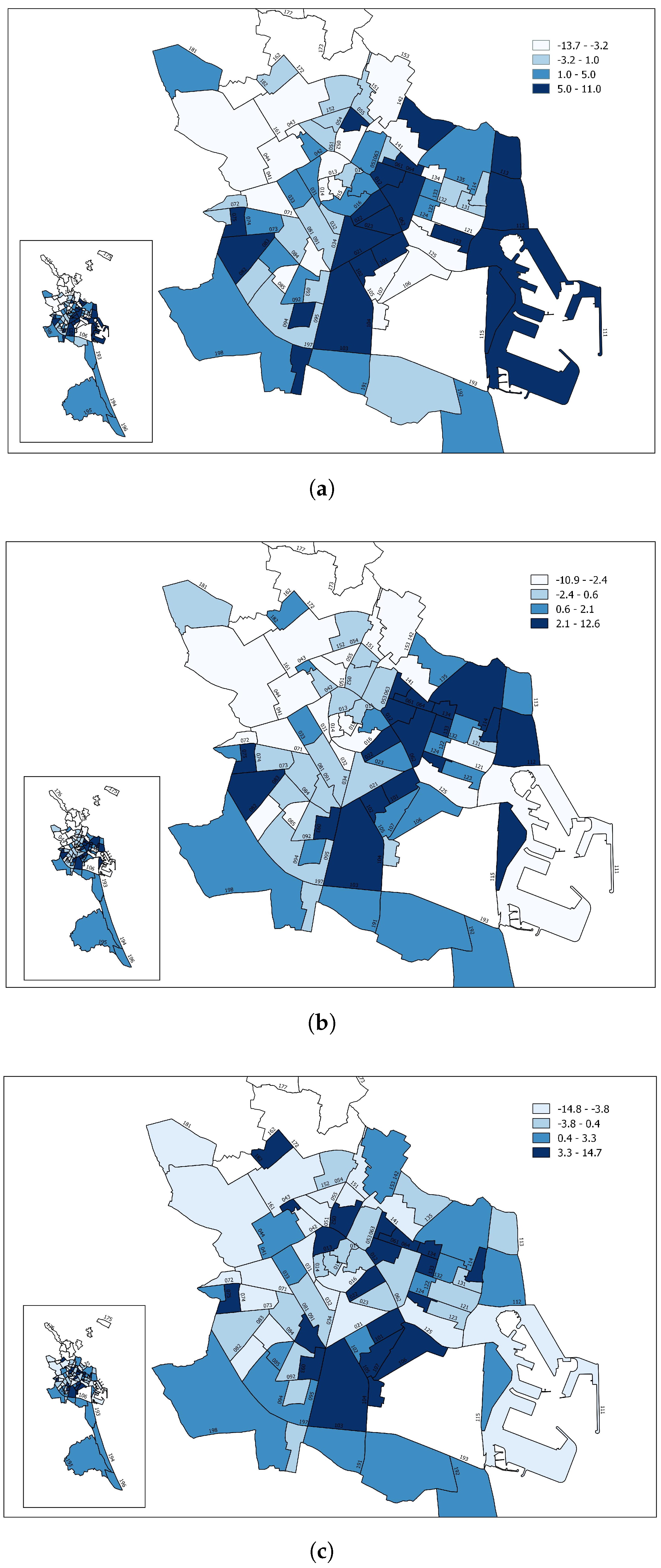
Figure 2 shows the changes in consumption differences with respect to the average resulting from the estimation of the mixed model for three different prices: the average price (
p = 3), a lower price (
p = 2) and a higher price (
p = 4). The maps thus show that a change in the average price meant that the relative consumption position of the neighbourhoods changed in some cases and remained unchanged in others. The difference between the average consumption of neighbourhood
k and the average of the whole city for each possible price is obtained from
(see
Table A3 in
Appendix A).
The total variance of the slope was equal to
(see
Table 1). If an average household had an estimated elasticity of −1.868, the 95% confidence interval for the elasticity was
, equal to [−1.21; −1.53]. Therefore, 95% of the sample households could be expected to have an elasticity between −1.21 and −1.53.
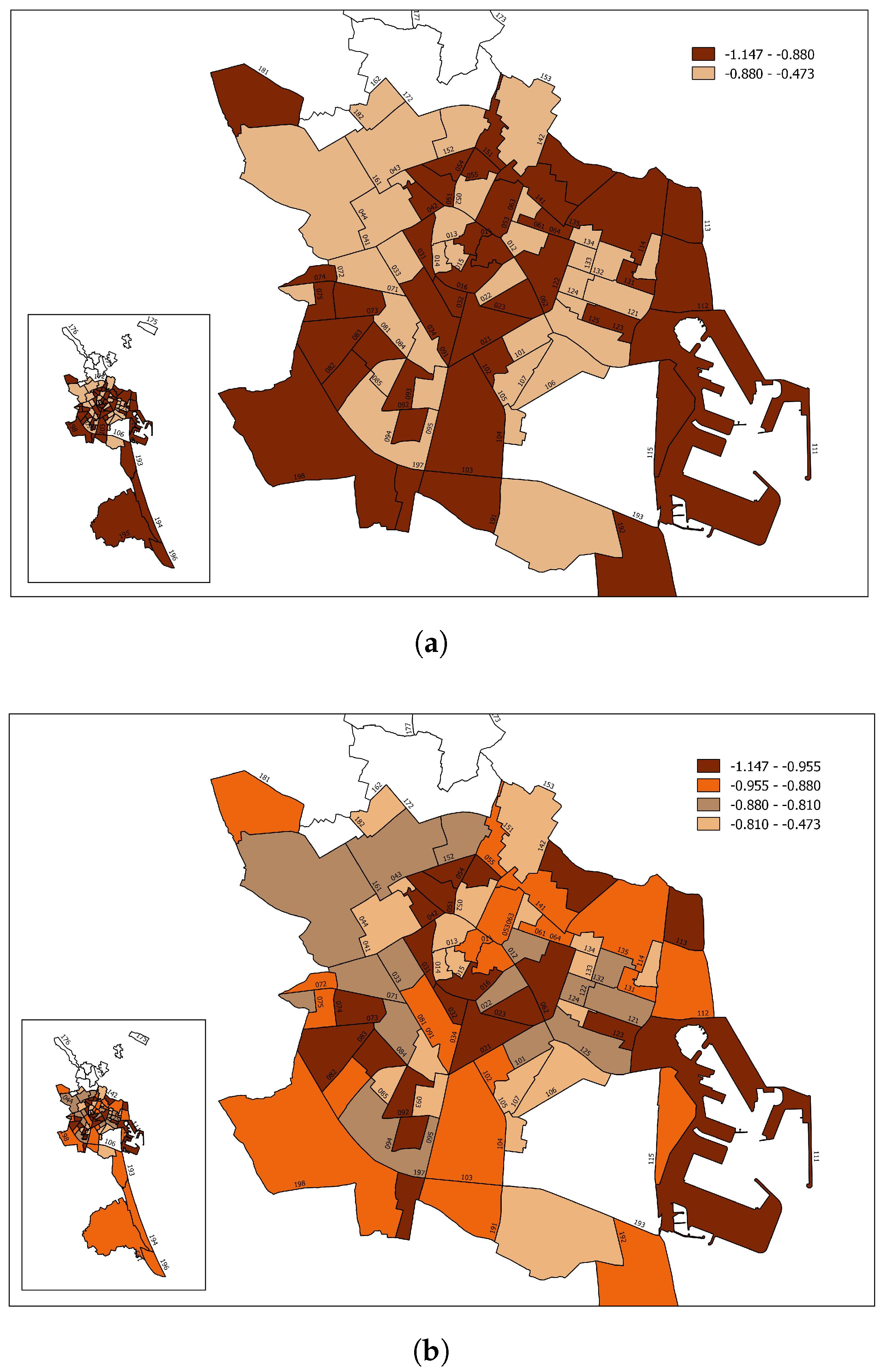
From the estimated values, it is possible to calculate the average elasticity of district
k for all periods as
(these values can be found in
Table A1 in
Appendix A). In
Figure 3, map
Figure 3a shows the elasticity values in two ranges that divide the districts into those with higher or lower than average elasticity. Map
Figure 3b represents four ranges.
The value of the average price elasticity for each neighbourhood depended on neighbourhood random effects, both in the intercept and in the slope. Although, for the average price (P = 3), the values of the neighbourhood elasticity were highly correlated with differences in consumption (i.e., neighbourhoods that consumed the least with respect to the average tended to be the most inelastic), this was not necessarily the case. For example, in L’Exposició neighbourhood (district 6), the random effect on the intercept was 0.07, and the effect on the slope was 0.05.
Hence, for P = 3, 12% more was consumed than the average for Valencia. However, the value of the elasticity for this neighbourhood was 0.815, which was below average (−1.868). The opposite case was that of Benimaclet neighbourhood (district 14). Here, the random effect of neighbourhood was divided between the intercept −1.009 and the slope −1.034 so that the difference in consumption with the average was −1.7% and the price elasticity was above average (−1.91).
After all, the differences in elasticity were due to the influence of random effects on consumption for each neighbourhood for a zero price (intercept) and the influence of neighbourhood random factors on the price sensitivity of consumers in that neighbourhood (slope).
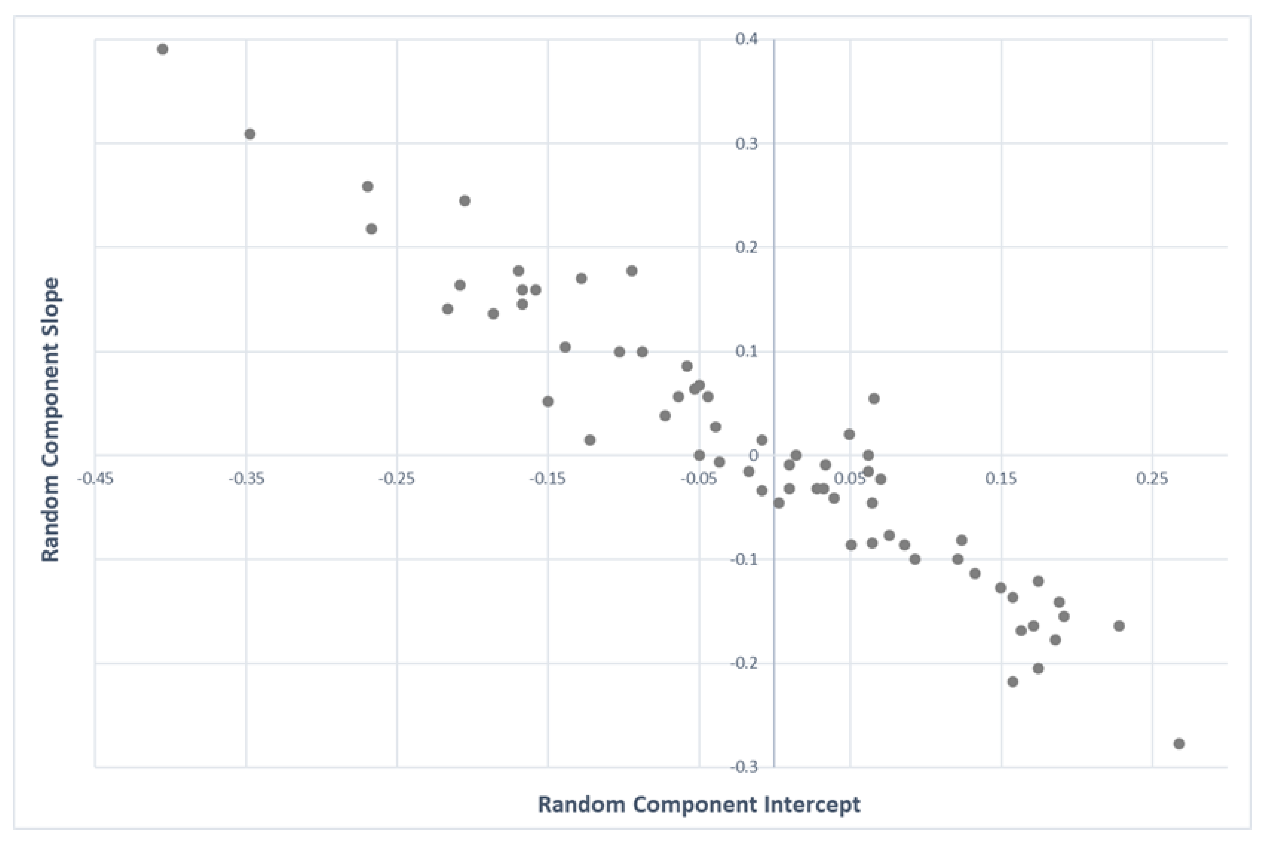
Additionally, an estimation of the covariance matrices measuring how the total variability was distributed across neighbourhoods, periods and observations was obtained: In the variances–covariances of the random effects for neighbourhoods (
Table 2), the covariances between the random terms of the intercept and the slope were negative. Thus, for the average price, a given neighbourhood had a smaller value of the random term of the slope if the random term in the intercept was larger (
Figure 4).
Neighbourhoods with a negative intercept (i.e., lower consumption than the mean for P = 0) tended to have positive slope components, which tended to have lower elasticities. Thus, consumption differences between neighbourhoods were not independent of price. Moreover, the fact that one neighbourhood consumed more than another for a given price does not imply that it consumed more at a higher or lower price.
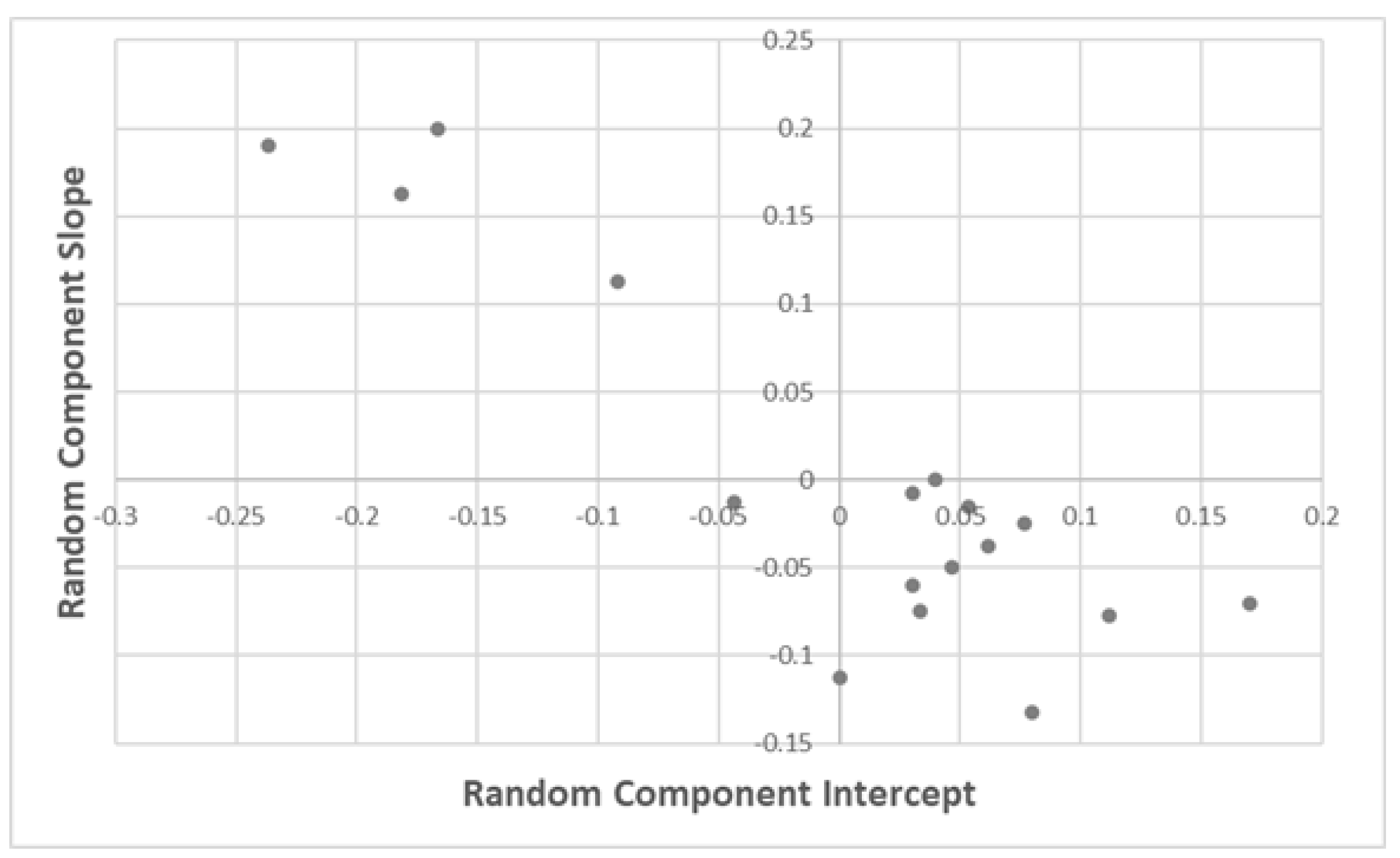
Regarding the covariances between the random effects on the intercept and slope for the period (
Table 2), as with the neighbourhood effects, the signs were negative. This implies that periods with a negative intercept tended to have positive slope components.
Figure 5 graphically shows the relationship between these random effects.
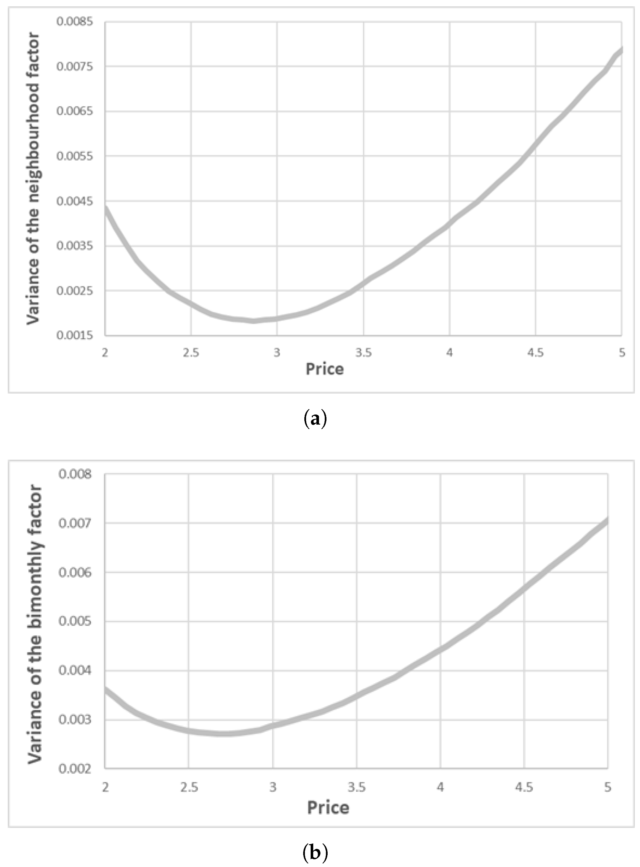
A consequence of the mixed model was to assume that the variance in neighbourhood water consumption depended on the average price they were paying. The total variability in consumption of household i in a model with random coefficients depended on the neighbourhood variance, the period variance and the idiosyncratic variance. Both the neighbourhood variance and the period variance depended on price in the following way:
Figure 6 shows these relationships.
Figure 6a shows how the variance in consumption between neighbourhoods reached its minimum near the average price (around 3 euros per m
3). Neighbourhoods that paid a price far from the average price had higher variability in consumption.
Figure 6b shows the part of the variance that corresponded to random time effects.
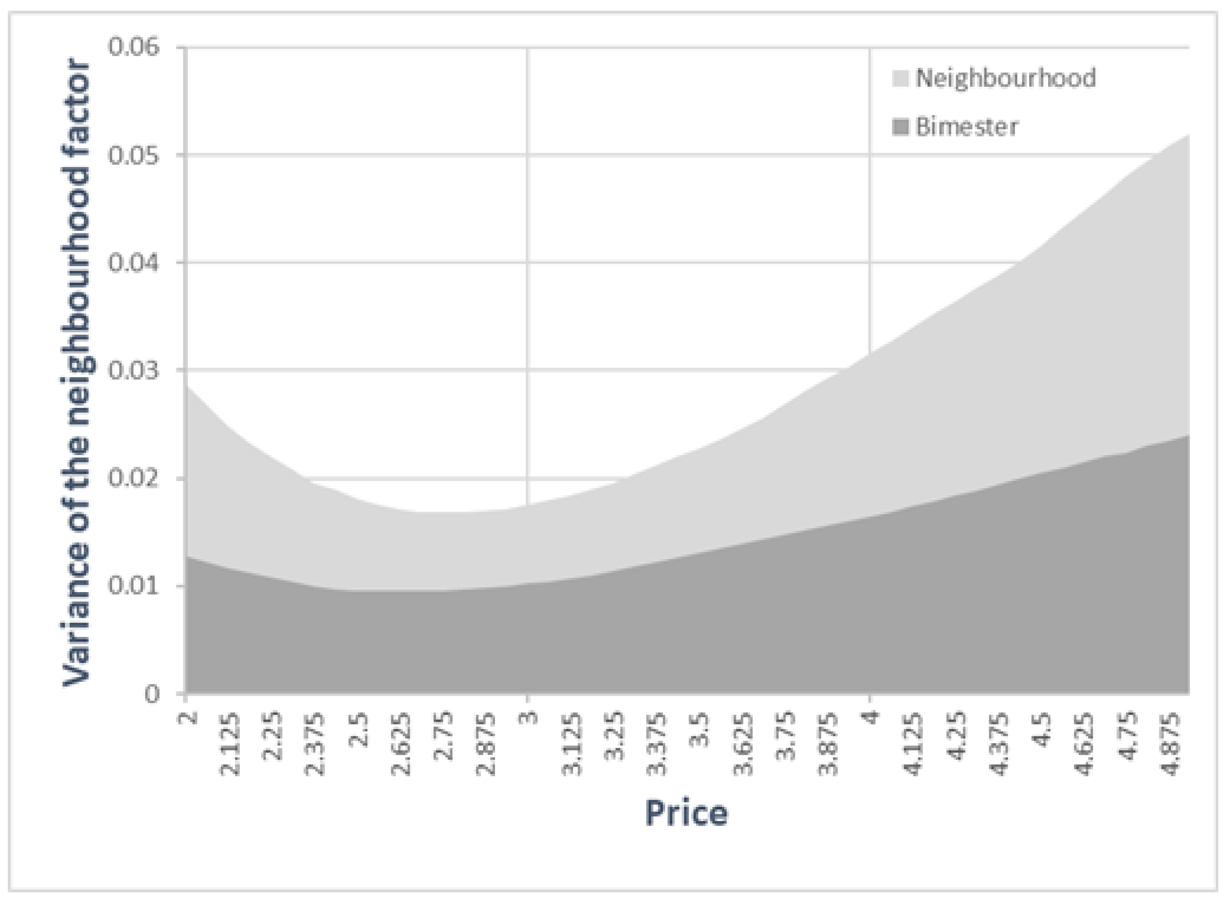
The consequence of the dependence of the variance between neighbourhoods on the price of water was that the variance partition coefficient (VPC) also depended on the price. Neighbourhoods where the water price was far away from the average price were also the neighbourhoods where the random effect was most relevant.
Figure 7 represents the part of the variance explained by the two random effects.
5. Discussion and Conclusions
The estimated elasticity for an average household is inelastic, with a value of −1.868. If the average price (total bill for one consumer divided by m
3 consumed) increases by 1%, this will result in a decrease in consumption of 0.87%. This value of the price-elasticity is in the range of the estimates obtained in the literature, although it is above the average values obtained in the main meta-analyses: Espey et al. [
9] reported an average price-elasticity of −1.51; Dalhuisen et al. [
10], of −1.41; Sebri [
11], of −1.37; Marzano et al. [
12], of −1.4; and Puri and Maas [
13], of −1.71. The higher estimated elasticity could be explained for several reasons related to the specifications and database used in the model.
Marzano et al. [
12] found, in the results of their meta-analysis, that the smaller the number of variables used in the demand specification, the higher the elasticity obtained. In this paper, the demand function estimated only included three independent variables, given the difficulty of obtaining socioeconomic data at the household level. On the other hand, the water price specification used in this paper (average price) also led to higher elasticity values compared to the use of marginal price. Additionally, double log functional forms were associated with higher demand elasticities.
Espey et al. [
9] and Dalhuisen et al. [
10] found that papers using micro-data had higher price elasticity values than those using aggregate data. However, Sebri [
11] found the opposite. Flores-Arévalo et al. [
23] analysed the effect of the level of data aggregation on the price elasticity of water demand. They found that the elasticity was higher for higher levels of data aggregation. However, the elasticity values were higher when panels of data were used in the analyses [
13].
The results have values and signs of parameters of surface area and persons per household in common with studies of the literature. The parameter estimate for the number of persons indicates that water consumption increased at a lower rate than household size. This could indicate the existence of economies of scale in consumption [
19,
79]. The evidence of the existence of economies of scale in domestic water consumption may justify changes in water price structures. Per capita consumption could be considered instead of per household consumption as well as changes in the special tariffs for large households [
58].
The value of the parameter related to the surface area of the dwelling showed a positive sign but less than one. Although this variable does not function as a proxy for household income levels, it can be assumed that there is a positive relationship between dwelling size and income levels (in our case, neighbourhoods with larger average dwelling size had higher average income levels). If this variable is considered as a proxy for income, these values characterise water as a necessary good. This result is highly relevant as they contain useful information for the design of water policies. They justify subsidies or aid to households with lower incomes to guarantee basic water consumption in situations of declining incomes.
The analysis also sought to verify whether consumer behaviour in different areas of the city was different and to what extent this was determined by place of residence. The results show significant differences in consumption across neighbourhoods compared to the city average. This variability in household consumption between neighbourhoods depends on an effect related to consumer behaviour in the neighbourhood for a zero price (i.e., whether people consume more or less than the city average regardless of price) and on an effect related to the price sensitivity of consumers in that neighbourhood. A 27% of the variability in consumption was explained by differences in household behaviour.
The estimations gave the value of the price elasticities for each of the neighbourhoods. The range of elasticities was between −1.21 and −1.53. Thus, water consumption depends on the spatial scale, and consumers in different neighbourhoods of the city have different levels of sensitivity to price changes. Moreover, households with the highest consumption have the lowest elasticities [
52,
81,
82].
This conclusion is reflected by the ranges of elasticities. The results are in agreement with those obtained by Pérez-Urdiales et al. [
79], in which a range of elasticities of −1.23 to 0.9 was found. Comparing these results with those of the other two papers that propose a mixed model to incorporate scale into the study of domestic water demand [
83,
84], the same conclusion was obtained, although the objectives of these two analyses were somewhat different from those of the present paper.
This study contributes to broadening the knowledge of the behaviour of drinking water. This type of research is important to capture unobserved heterogeneity between individuals and local differences in domestic water consumption at the intra-urban level. More studies using methodologies that allow capturing heterogeneity in consumption at a scale below the municipality are necessary, since studies such as this one can provide managers with knowledge that can help them apply different economic instrument, prices and taxes to the urban water demand of different types of users.
In terms of future lines of research, to overcome unobservable heterogeneity, the domestic water demand function could be estimated using a quantile regression model. With the analysis of the domestic water demand using a quantile regression model, consumers could be divided into quantiles that represent their water consumption levels, and their behaviour could be estimated depending on the quantile. Through this methodology, it would be possible to analyse consumer behaviour within each neighbourhood to capture the heterogeneity between individuals and between neighbourhoods. The estimation of this model gives both the consumption differences in levels and the elasticity differences of each consumer group.


