Automatic Open Water Flood Detection from Sentinel-1 Multi-Temporal Imagery

Abstract

Many technical infrastructure operators manage facilities distributed over large areas. They face the problem of finding out if a flood hit a specific facility located in the open countryside. Physical inspection after every heavy rain is time and personnel consuming, and equipping all facilities with flood detection is expensive. Therefore, methods are being sought to ensure that these facilities are monitored at a minimum cost. One of the possibilities is using remote sensing, especially radar data regularly scanned by satellites. A significant challenge in this area was the launch of Sentinel-1 providing free-of-charge data with adequate spatial resolution and relatively high revisit time. This paper presents a developed automatic processing chain for flood detection in the open landscape from Sentinel-1 data. Flood detection can be started on-demand; however, it mainly focuses on autonomous near real-time monitoring. It is based on a combination of algorithms for multi-temporal change detection and histogram thresholding open-water detection. The solution was validated on five flood events in four European countries by comparing its results with flood delineation derived from reference datasets. Long-term tests were also performed to evaluate the potential for a false positive occurrence. In the statistical classification assessments, the mean value of user accuracy (producer accuracy) for open-water class reached 83% (65%). The developed solution typically provided flooded polygons in the same areas as the reference dataset, but of a smaller size. This fact is mainly attributed to the use of universal sensitivity parameters, independent of the specific location, which ensure almost complete successful suppression of false alarms.

1. Introduction

Satellites equipped with a synthetic aperture radar (SAR) are being used in various applications utilizing an analysis of signal backscatter intensity and eventually its change in time. An indisputable advantage of this active microwave technology is the ability to work at any time of the day and under any meteorological conditions. Satellite-based flood detection is one of the applications which can enormously benefit from this advantage as optical imagery often suffers from high cloud coverage during flood events.

The flood detection from SAR imagery is based on the fact that the SAR signal backscattered by water bodies has a very low intensity. Therefore, a SAR intensity threshold allowing the pixels representing the water surface to be distinguished from others (mainly corresponding to land) is sought in most of the references (such as [1,2,3]). Hereafter, we call this threshold a water–land threshold. According to the cited references, the threshold, which depends on many factors, including meteorological conditions (wind, temperature), differs for each image, and has to be estimated from the evaluated data. The estimation of this water–land threshold is, therefore, a crucial part of the algorithm.

To estimate this water–land threshold, authors in [2,3] firstly used a method based on a bimodal histogram. To handle cases where only a small part of the AOI is flooded, they divided the AOI into tiles and searched for the threshold in each tile individually. We suppose this tiling method is suitable for very high-resolution imagery (such as TerraSAR-X for which it was developed) and the evaluation of solely flood images: in the case of a small flooded area, bimodal histograms are not guaranteed.

Several algorithms or even complete processing chains for automatic flood detection from SAR imagery have been presented to date. In 2009, Martinis et al. in [1] reported the successful development of a near real-time (NRT) flood detection solution from high-resolution TerraSAR-X data. Split-based histogram thresholding and segmentation-based classification formed the basis of this approach. It was more recently substantially refined and extended as described in [2]. Very high-resolution X-band SAR images were also used to test a solution developed by utilizing fuzzy logic and auxiliary data in the classification step [4].

The deployment of the Sentinel-1 mission, delivering a reasonable and uniform revisit acquisition time increased effort in this area. Firstly, Twele et al. in [3] adapted the solution presented in [2] for this satellite system. The authors in [5] tried to improve histogram thresholding using bilateral filtering as a smooth labelling method and tested the approach on three European events. The authors in [6] used the Otsu iterative thresholding algorithm applied to Sentinel-1 GDR data with single VV (vertical transmit-vertical receive) polarisation. Another approach is mentioned in [7]. It is based on a normalized difference ratio comparing pre-event and post-event images, using both VV and VH (vertical transmit and horizontal receive) polarisations. Furthermore, more recently, automatic flood detection algorithms were developed from Sentinel-1 imagery based on neural networks [8,9], kernel algorithms and machine learning [10], or alternating decision trees [11].

Although radar satellite remote sensing (RS) is mainly used to detect open-water flooding in rural environments, some authors dealt with possibilities to use it in urban areas [12,13,14,15,16,17,18]. Moreover, authors in [19,20,21,22] worked on the detection of flooded vegetation.

Some authors were applying a fusion of SAR imagery with other types of data, such as optical imagery [7,17,23,24], LiDAR [9], WorldDEM [18], land cover [25], the shuttle radar topography mission (SRTM) digital elevation model [25], or flood hazard maps [14,26].

For more detailed information about the state-of-the-art of using SAR imagery for flood detection and mapping, the reader is referred to [27].

Most of the studies mentioned above were performed only to evaluate a specific event or a limited set of events. Only study of Yang et al. was broader, covering the continental part of the USA for three and a half years [10]. However, even this study was tied to US- specific conditions. The developed system was closely linked to other existing structures in the USA, such as the United States Geological Survey, a network of gauge stations, etc. Some other solutions, e.g., [6,7,8,9,10,11,13,14,17,18,24,26], relied on the use of computational intelligence tools, indexes and thresholding, or on specific auxiliary data sets. The computational intelligence tools used, such as neural networks, must always be trained on sample data first and only afterwards can be used to evaluate the current situation. Their disadvantage is that the training data set binds them to a specific geographical area and spatial or spatiotemporal context. However, they may not work properly in another spatial context. Other methods (e.g., indexes and thresholding) have been mostly tuned to work best in the test area.

The auxiliary data sets used often do not have global coverage, and thus the use of the procedures developed over them is also geographically limited. It is impossible to use them in any place and at any time.

None of the studies mentioned above offer an assessment of the performance of the developed system over a long time period, especially with respect to so-called false positives, i.e., cases when flooding was identified by the system but did not happen in reality. These false positives can happen, e.g., due to agricultural works or seasonal changes.

The solution proposed in this paper is an attempt to overcome these barriers. Our goal was to develop a method that can be applied anytime and anywhere, not dependent on training, using only a minimum auxiliary data which will also have a global validity.

We developed an automated processing chain for NRT open-water flood detection based on Sentinel-1 imagery which can be run in an on-demand or permanent monitoring mode. When the solution is implemented, automatic notifications for a given area of interest (AOI) can be provided to a user without any need for an intervention or manual steps from his side. It can be beneficial mainly for stakeholders who operate infrastructure over vast or distant areas and want to be warned about potential threats or damage to their facilities.

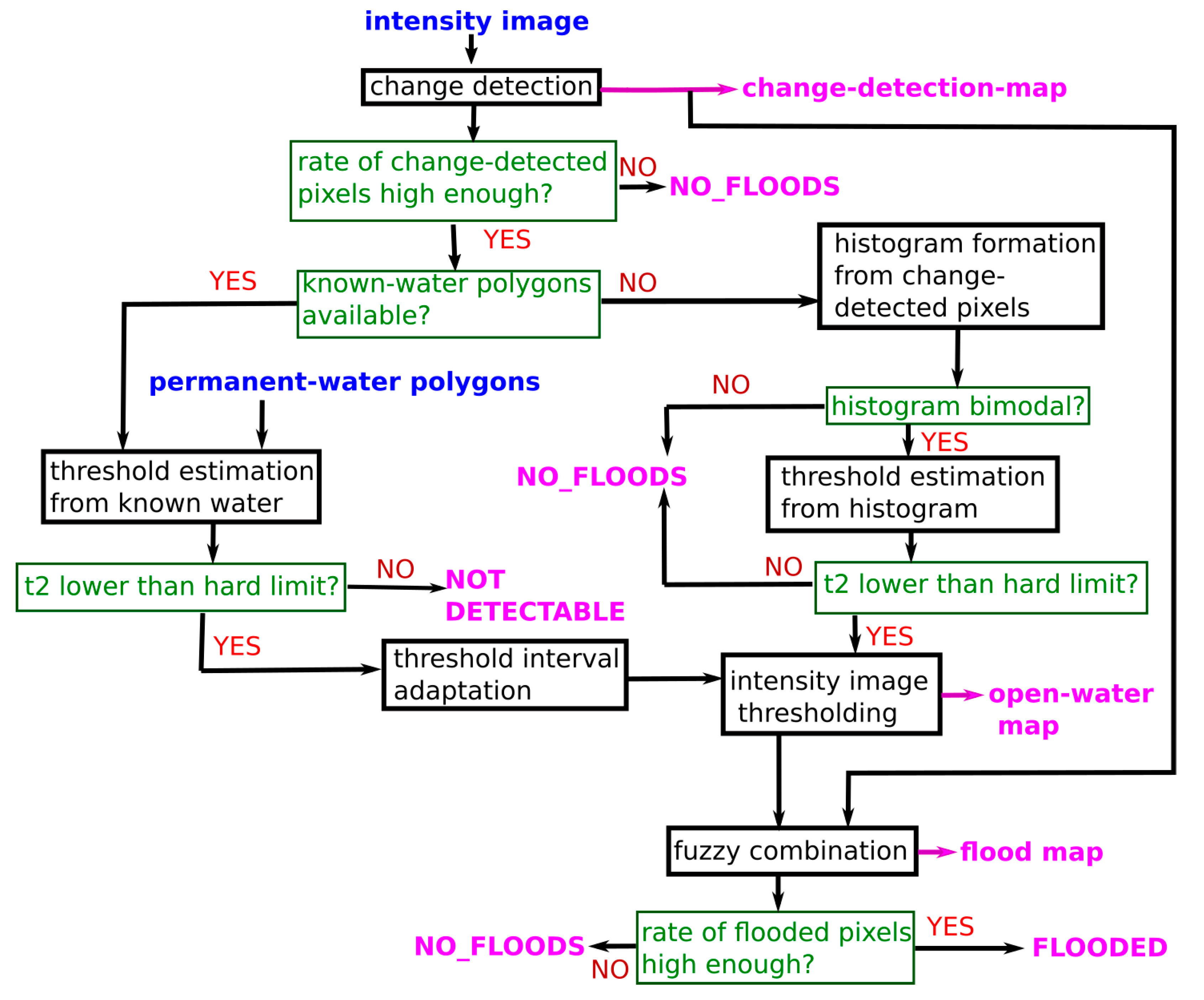
The developed solution is based on a combination of two separate algorithms utilizing Sentinel-1 images to suppress false positives and to enhance the quality of the flood detection results. The first algorithm addresses the detection of areas where a statistically significant change in backscatter intensity happened compared to the previous state. The second algorithm, inspired by [1,2,3], applies thresholding to the backscatter intensity to find open-water flooded pixels and includes fuzzy and region growing approaches in the classification process. Although multi-temporal change detection and intensity thresholding was previously combined by [28], this is the first time it was performed in an automatic processing context. After a detailed description of the developed solution, the results from processing long periods, including several flood events in Austria, Germany, the Czech Republic and Italy, are demonstrated, and the potential limits of the developed solution are discussed.

2. Data

2.1. Data Used for Flood Detection by the Developed Solution Based on SAR Imagery

The solution is designed for permanent, automatic monitoring using all available Sentinel-1 data. In Europe, the acquisition period is usually six days (some images can be missing). For a defined AOI, images from all available data track geometries are automatically downloaded from a user specified data repository. The input of our algorithm is Sentinel-1 data with resolution of 10 × 10 m and precise orbits applied, radiometrically calibrated into γ0 [dB] and spatially filtered using a 7 × 7 improved Sigma-Lee filter [29].

Each track was processed separately, leading to three to four individual flood maps, which were evaluated independently. For each AOI, the number of processed Sentinel-1 images is in the order of tens or hundreds, depending on the length of selected time period.

If the water–land threshold (see Section 3.1.2) is to be estimated from permanent water bodies, the user must provide a polygon layer with water bodies within or near the AOI. The developed solution uses no other auxiliary data.

2.2. Data Used for the Preparation of Reference Datasets for Validation of the Developed Solution

The solution developed for open water flood detection was validated on five different flood events within the Czech Republic, Germany, Austria and Italy. Depending on the specific flood event, the following data sources were used as a reference dataset or for its creation:

• Satellite optical imagery acquired during or early after the flood event.
• Flood delineation product provided by the Copernicus Emergency Management Service (EMS).
• Own photo documentation from the localities.

The exact source of the data used to create a reference dataset for a specific evaluated flood event is always mentioned in the pertinent part of Section 4, which contains the validation results.

When satellite optical imagery was used to prepare the reference dataset, the extent of flooding was manually digitized using compositions in true or false colours and the NDWI (normalized difference water index) index. A polygon layer with a delineation of the flood extent was therefore created.

3. Methodology

3.1. Flood Detection Processing Chain Methodology

The workflow of the developed solution can be summarized in the following steps. For the Sentinel-1 data specified in Section 2.1, the change detection with regard to older data is performed first. If the number of change-detected pixels is very low, no floods are detected and the processing stops. As the second step, land-water thresholds are estimated from the data, either using permanent water polygons, or the histogram bimodality method. Then, these thresholds are adapted and the SAR image is converted to the open-water fuzzy map. Finally, the change-detection map is fuzzy-combined with the open-water map, and according to the number of non-zero pixels, it is decided whether or not the image should be classified as FLOODED.

The described processing chain is designed to be rerun when a new image is acquired. The change detection then compares the new image with an updated stack of older images. A flowchart of the designed processing chain is displayed in Figure 1. Individual steps of the processing chain are described in detail in the following sub-sections.

3.1.1. Statistical Change Detection

Statistical change detection is applied to the evaluated image to find pixels whose backscatter intensity significantly changed compared to the past. The past is established based on comparing the mean over a reference stack containing the last five images (one month) with the current image, and also considering the standard deviation within the reference stack. A statistical test of identity is performed pixel-wise with the null hypothesis being that current image is identical to the previous ones. The test result is a real value where 0 corresponds to no change and −1/1 values correspond to the limit situation where the difference exactly corresponds to the critical change value. Higher positive or smaller negative values indicate more significant changes. The sign of the change (increase or decrease of the intensity) is preserved, and the real value of the change detection output lets the user more finely tune the significance of the change required to detect floods.

The change-detection statistics are then spatially filtered in a user-defined window to suppress noise, and the “SS” fuzzy function (see Figure 2b) is applied to it, resulting in a change detection significance map. The result of the statistical change detection is then a fuzzy value in the (−1, 1) interval, preserving the sign of the change (positive: increase of SAR intensity, negative: decrease of SAR intensity). Finally, inspired by [2,3], the region growing approach is applied to remove small patches and patches with low significance, highly probably corresponding to noise.

If the number of change-detected pixels is very low (i.e., below 0.1 % of the total number of pixels in the AOI), the flood detection processing is stopped at this step with the results of “NO FLOODS”.

3.1.2. Water–Land Fuzzy Thresholds for Open-Water Detection: Estimation and Adaptation

The water–land threshold estimation is the critical step of the whole algorithm. It must be run independently for each image. We implemented two methods for the water–land threshold estimation: one (A) based on bimodal histograms with a limited number of pixels, and the other (B), requiring additional data.

(A) In order to obtain bimodal histograms to estimate water–land thresholds with higher probability (for flood cases), we combined the intensity thresholding with a statistical change detection: the histogram to estimate the water–land threshold is formed only from the change-detected pixels. The change detection process was described in Section 3.1.1.

The advantage of this method is that it does not require any additional data. Nevertheless, the reliability of the bimodal histogram algorithm is still questionable for permanent monitoring due to the occurrence of bimodal histograms after agricultural works on large areas (with regard to the AOI). Unfortunately, intensity thresholds obtained from these “agricultural” bimodal histograms are sometimes low enough to be comparable to real water–land thresholds.

(B) More robust land-water threshold can be estimated based on neighbouring permanent water bodies. It is preferable if the permanent water bodies are (1) large, so they contain many water pixels with a smaller number of edge pixels, possibly corrupted by vegetation or non-water surface, and (2) close to the investigated AOI, so the meteorological conditions are as similar as possible.

In (B), we also form a histogram; however, it is based only on pixels representing permanent water bodies. This method requires the permanent water bodies to be defined. Polygons with permanent water bodies from publicly downloadable free sources can be used. However, due to their potential limited geometry precision, applying a negative buffer on them before their use is advised to decrease the number of pixels corresponding to non-water areas.

In order to apply method (B) for water–land threshold estimation, our solution often needs to process a larger area than AOI alone (easily achieved with Sentinel-1 data) to cover these permanent water bodies.

Our algorithm primarily estimates the intensity thresholds based on permanent water bodies (method (B)). If they are not available (either the area of water bodies was not processed, or the polygon layer is missing), the histogram bimodality method (A) is used to estimate the intensity threshold. The reliability of the two methods differs significantly.

In order to apply the fuzzy approach (inspired by [2,3], allowing us to evaluate the certainty of detection), two thresholds are needed: the lower threshold t₁, indicating the highest SAR intensity of “certain water”, and the higher threshold t₂, indicating the lowest SAR intensity of “no water” (Figure 3).

The authors in [2], applying the histogram-bimodality method (A), recommend setting the lower fuzzy threshold t₁ to the maximum of the peak representing water, and the higher fuzzy threshold t₂ (corresponding to zero probability of water) to the minimum between the two peaks, as illustrated in Figure 3a. In the histogram bimodality approach, we follow this recommendation.

In the permanent-water approach (method (B), we use the histogram maximum as the lower fuzzy threshold. The higher fuzzy threshold is estimated as a histogram quantile (e.g., 85%), discarding points with the highest intensity as these can correspond to the water banks, vegetation etc., and deteriorate the water detection results.

In addition, a hard limit of around −15 dB for Sentinel-1 imagery is posed on the higher fuzzy threshold t₂ (see Figure 4a) for both methods. For method (B), if the estimated water–land threshold is higher, the processing results in “NOT DETECTABLE” status due to weather or other conditions. Such a high value is usually caused by strong winds leading to waves on large permanent water bodies or by ice covering them, and in such cases, it is impossible to distinguish water and land areas based on SAR imagery. For method (A), the processing results with “NO FLOODS” status as the histogram minimum do not necessarily need to correspond to the real water–land threshold.

According to our experience, the interval between the two fuzzy thresholds varies significantly among the acquisition dates (in the range of about 0.5–5 dB), leading to a nondeterministic behaviour regarding flood detection. Therefore, our algorithm adjusts the interval between the two thresholds (with the lower threshold t₁ (see Figure 4a) remaining constant). The interval is adjusted in order to be within a given narrow interval (3–4 dB) if it is possible concerning the above described hard limit (see Figure 4 for illustration). This approach gives better results in comparison to widening the interval by a multiplicative constant.

The “Z” fuzzy function (see Figure 2a) with the two intensity thresholds t₁ and t₂ is then applied to the current SAR image, the result is spatially filtered (3 × 3 window), and a region growing approach is applied in order to remove too-small areas. The result of this operation is an open-water fuzzy map with values in the (0–1) interval, with 0 for no water, 1 for certain water (floods + permanent water bodies), and other values for areas where the occurrence of water is possible but not certain. In comparison to [2,3], the minimum number of neighbouring flooded pixels is set to 5–10 (allowing to detect flooded areas of a scale of about 1000 m²).

3.1.3. Combination of the Change Detection and Open-Water Detection

The change detection and open water fuzzy maps are combined using pixel-wise fuzzy combination in the last step. According to Martinis et al. in [2], they are defined as the average of two values if they are both non-zero and zero in case one of the values is zero. The result of this combination is a so-called flood map.

If the flood map is non-zero for more than 1% of the AOI, the algorithm returns the status “FLOODED”. In the case of a smaller non-zero area, such an area is considered a false positive, and the algorithm returns the status “NO FLOODS”. The resulting status is essential for deciding whether to notify an operator in order to take appropriate measures.

3.1.4. SAR Polarizations

The Sentinel-1 satellite acquires imagery in two polarizations: VV and VH. Studies [3,24] recommend using VV polarization for flood detection. Using solely VV polarization led to a high number of false-positive detections in our experiments, particularly during the spring season. On the other hand, using solely VH polarization led to a high number of false-positive detections generally (see Section 4.7). In both cases, they occurred mainly on agricultural land.

In order to reduce the number of false-positive detections, the algorithm uses both data polarizations: the processing chain (see Figure 1) is run independently for each of them, and finally, the states are combined. In order to result in “FLOODED”, the state “FLOODED” must be the result of runs in both data polarizations. To provide the final flood detection product, the one-polarization flood maps are fuzzy-combined in the same way as described in Section 3.1.3.

The parameters of the algorithm (thresholds t₁, t₂ for change detection influencing sensitivity, intensity hard limit etc.) are individual for each polarization.

The requirement for the floods to be detected in both polarizations simultaneously led to a significant reduction in the number of false-positive detections. On the other hand, the area of the resulting flood-detected areas was often underestimated, usually due to open-water detection in VH polarization. Therefore, as a final step, the fuzzy combination of flood detection results from both polarizations is realized in the following way. If the floods are detected from both polarizations on a significantly high number of the same pixels (i.e., on more than 0.1% of AOI), the fuzzy combination is calculated as the pure average of both polarizations.

3.1.5. Reference Image Stack

As already mentioned, the processing chain is designed for permanent continuous monitoring of a given AOI, and the change detection step (see Section 3.1.1) uses five past images as a reference. Initially, the five oldest images in the series are taken as a reference, and the sixth image is evaluated. After evaluating an image, it is decided whether the evaluated image can be passed to the reference stack: only “NO FLOODS” images are passed. If a new image is passed into the reference stack, the oldest image from the stack is dropped. Therefore, the number of images in the reference stack is constant, but their time span is not, especially in flood seasons and in the seasons of frequent agricultural changes. Reference stacks include only images that were classified “NO_FLOODS” in both polarizations.

This approach may generate problems in cases of long periods of floods or unfavourable meteorological conditions, as a temporal gap can arise between the current image and the reference stack, while the AOI might change significantly during this gap.

3.2. Methodology of Flood Detection Validation

The developed solution for open water floods detection was validated on five different flood events within the Czech Republic, Germany, Austria and Italy. Besides that, it was also run in a rural area of South Moravia where no floods were expected to happen during the evaluated period to test the occurrence of false-positive alarms due to agricultural works.

The following approach was applied in the validation process:

• Process longer periods of data from ascending and descending tracks in the selected AOI with the developed flood detection solution (typically from March till November),
• Prepare an overall assessment for the whole processed period to evaluate detection of floods in proper epochs and the existence of false-positive alarms,
• Prepare a detailed assessment during a period of real floods to evaluate the quality of flood delineation with the comparison of results based on a reference dataset. Polygons identified as flooded from the used reference dataset were converted to a binary raster representation with two classes: (a) open water area and (b) other areas. Similarly, raster flooding maps provided by the developed solution were re-classified into the same two classes. All pixels identified as flooded were classified as open water area, regardless of their flooding probability. In the next step, standard classification metrics were computed to statistically compare results from both sources.

4. Experimental Results

Validation results from four European countries, including five flood events, are presented separately in the following sub-sections. As the processing chain was developed for an automatic operation without user intervention in any given AOI, identical settings of flood detection parameters were used for all evaluated events and areas. No fine-tuning of these parameters for specific areas or flood events was therefore applied.

4.1. Germany, Lower Saxony, Summer 2017

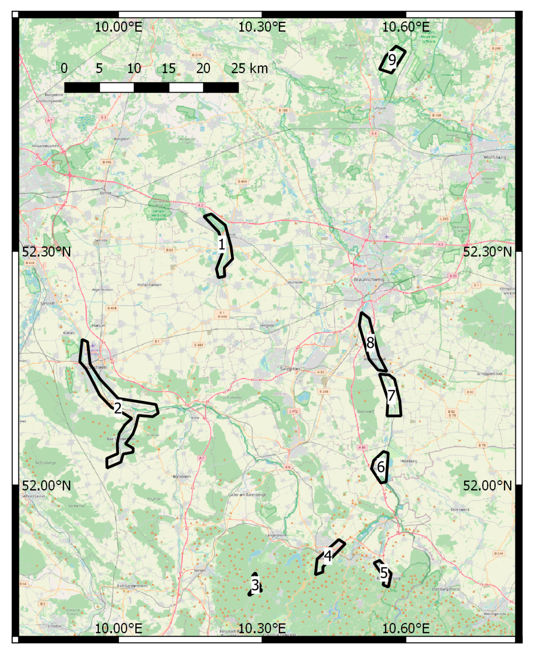
An extensive flood event on 25 July–30 July 2017 happened in southern Lower Saxony close to the cities of Hannover, Hildesheim and Braunschweig. This territory is mainly constituted of lowlands. Hydrological report of the flood event is provided in [30]. Based on the available sources, nine separate sub-areas with a total surface area of 97 km² (see Figure 5) were selected for validation. The localities were selected in order to test the developed solution in a diverse set of conditions. Some of them are constituted mainly by a rural land cover (agricultural fields, meadows); others mainly by urban areas in which the developed solution was not expected to work. The officially reported level of flooding in the selected sub-areas correspond to a return period from 20 to 200 years depending on the locality [30], but was unfortunately not specified for some of them (n. 3, 4, 5, 8).

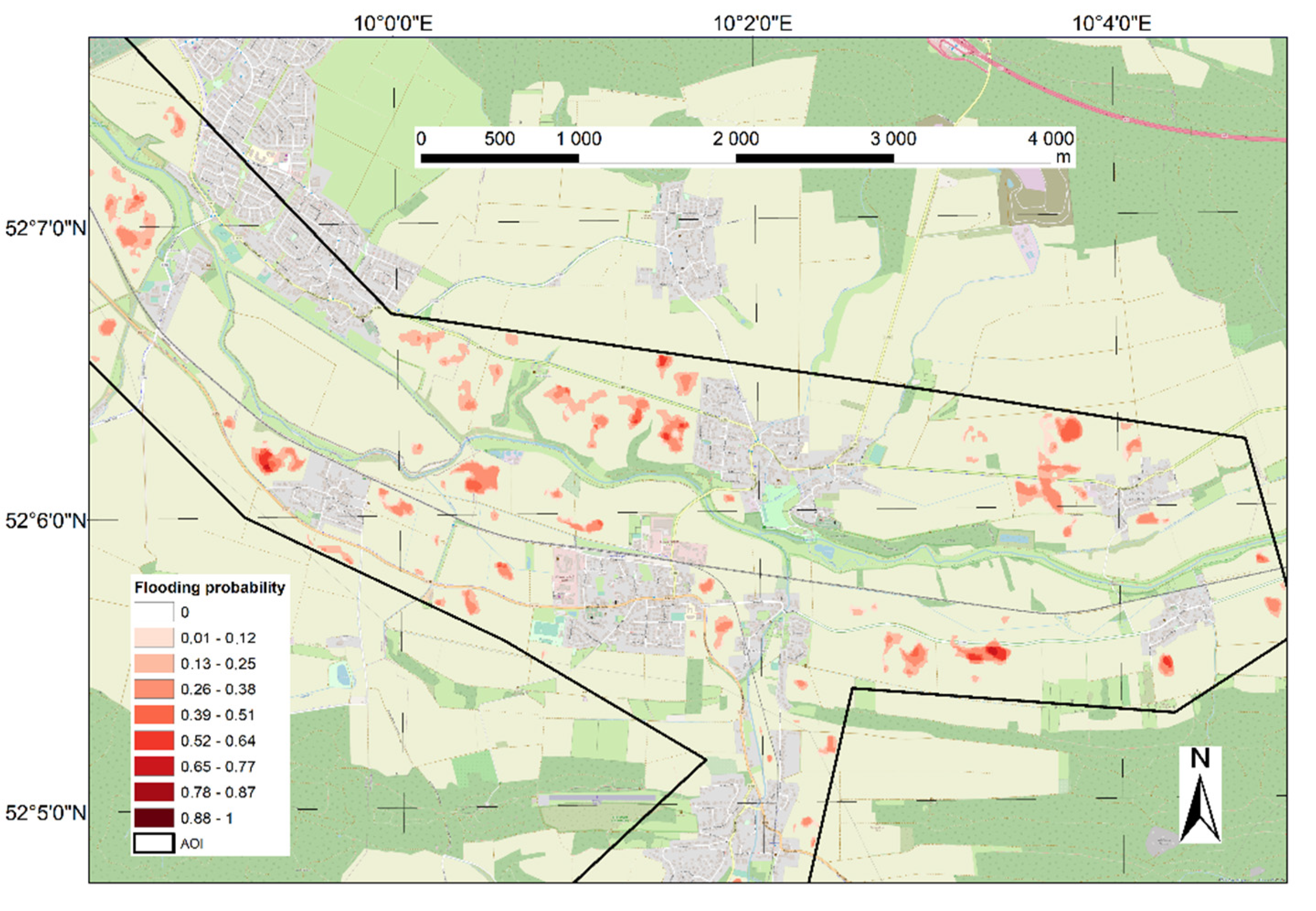
Sentinel-1 data from one ascending (A117) and one descending track (D66) were processed with the developed solution from the beginning of March until the end of November 2017. The evaluated flood event was correctly identified in five sub-areas with rural landscape, all from both processed tracks. The flooding was not identified in four urban sub-areas (n. 3, 4, 5, and 6). In terms of false positives, there were only three events in total within all nine sub-areas during the whole processed period. An example of false positive flood detection in sub-area two is shown in Figure 6. Similar to the other two false-positive events, the majority of the areas wrongly detected as flooded were located on agricultural fields.

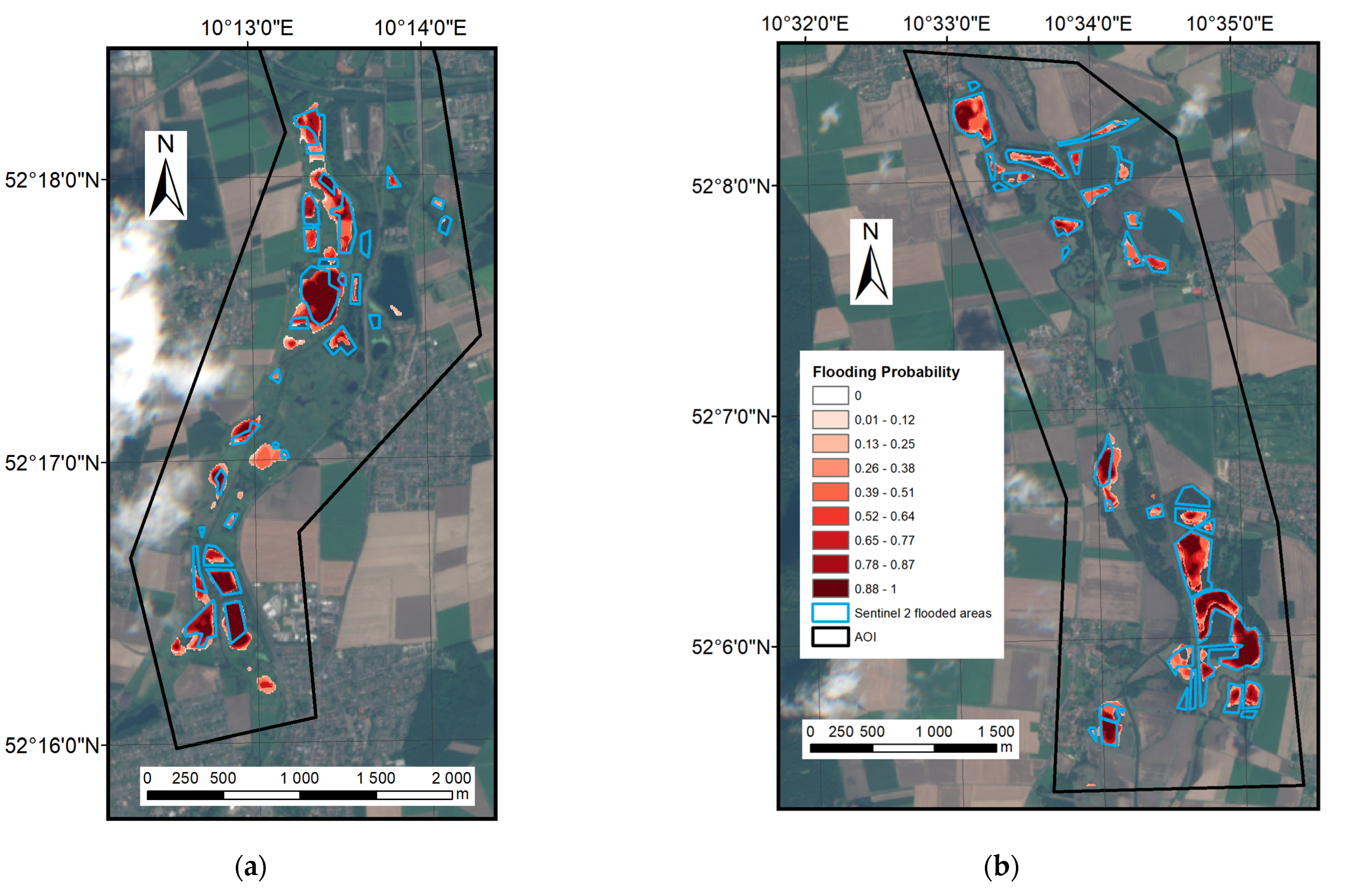
The outputs of the developed solution were compared with a reference data set to assess its performance in detecting the extent of real flooding. The reference dataset was based on Sentinel-2 images acquired on days of flooding or shortly after. In sub-areas 3, 4, 5, and 6, no flooding was identified from the Sentinel-2 images acquired on July 29 or on July 31. These are the sub-areas in which the flooding was also not detected by the developed solution. Figure 7 shows the extent of flooding from both sources for the selected sub-areas 1 and 7. It is apparent from the figure that the flooded polygons detected by the developed solution (in red) correspond well to the flooded polygons obtained from the reference Sentinel-2 imagery (in blue). A similar situation was found in the case of all other sub-areas with detected flooding.

Table 1. Statistical evaluation of comparison between flood extent detected by the developed solution and digitized from Sentinel-2 imagery for the Germany 2017 event. OA—overall accuracy, PA—producer accuracy, UA—user accuracy.

Sub-Area	OA (%)	PA Open Water (%)	UA Open Water (%)	PA Other (%)	UA Other (%)	Kappa Coefficient
1	96.7	67.4	54.8	97.9	98.7	0.59
2	99.0	70.4	90.7	99.8	99.2	0.79
3, 4, 5, 6	floods not detected from Sentinel-1 and Sentinel-2 imagery
7	96.2	66.4	86.0	99.0	96.9	0.73
8	98.4	57.9	74.8	99.5	98.9	0.64
9	96.1	68.0	82.8	98.7	97.1	0.73
Mean	97.3	66.0	77.8	99.0	98.2	0.70

contains statistical evaluation between the results of the developed solution and the flooding extents derived from the reference dataset. Overall accuracy (OA) represents a percentage of all pixels classified correctly, producer accuracy (PA) for open water is the probability that an area identified as flooded in reference dataset was flooded in reality. Similarly, user accuracy (UA) for open water represents the probability that an area identified as flooded by the developed solution was flooded in reality. Mean OA reached 97.3%, mean UA (PA) for open water was lower with 77.8% (66.0%) and varied for individual sub-areas. Lower values of PA compared to UA indicate that flooding was detected on a higher number of pixels from reference Sentinel-2 imagery than by the developed solution. The reasons for this situation are discussed in Section 4.

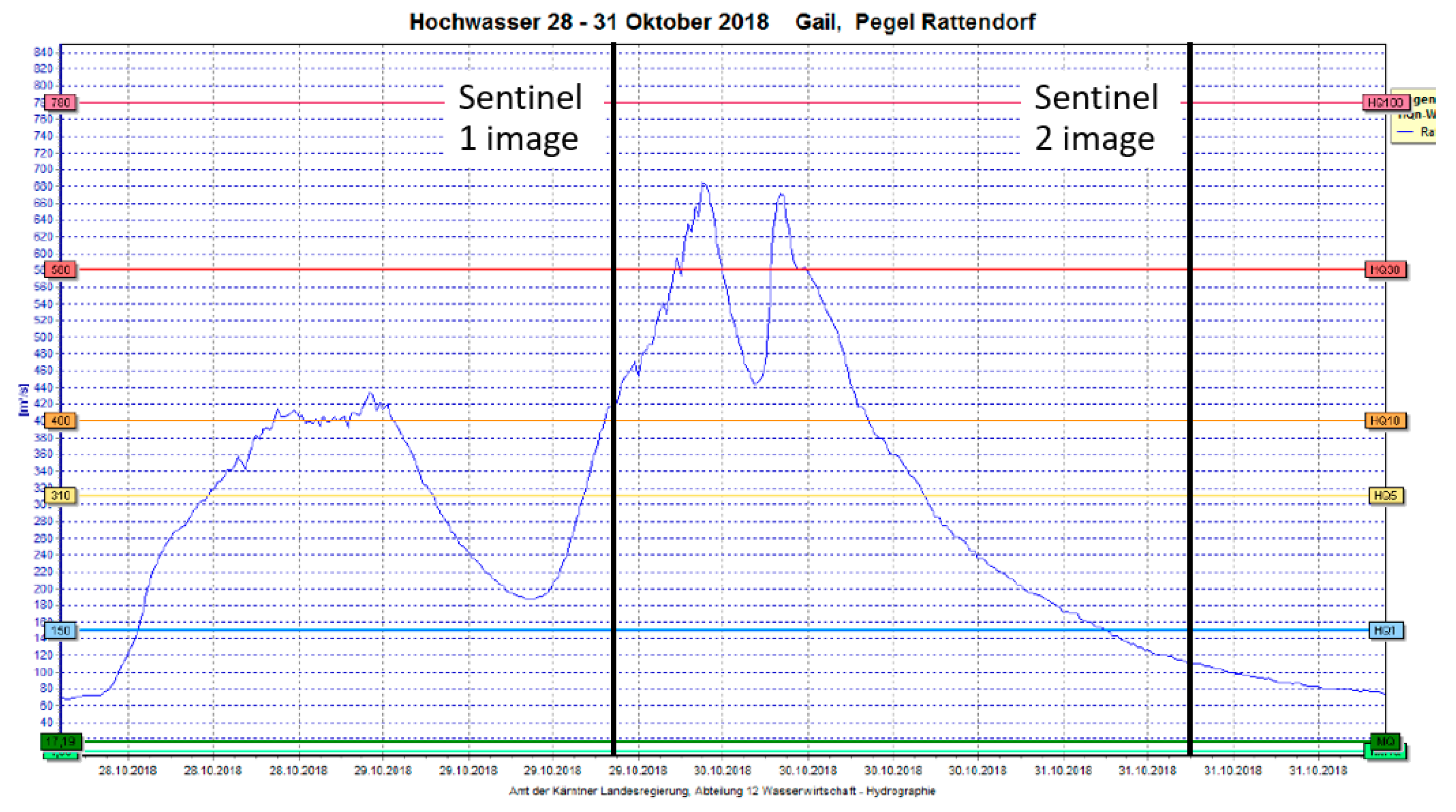
4.2. Austria, Southern Carinthia, Autumn 2018

From 28 October to 31 October 2018, flooding took place in the southern Carinthia region of Austria, west of Villach city. The floods mainly affected several valleys in the local Alps and consequently areas in lower parts of affected water streams. A general overview of the event is available in the hydrological report [31]. For validation, the mountain valley lying on the Gail river was chosen for which officially reported flood levels ranged between the 45 and 115 years return periods. Meadows are the prevailing landscape in the selected 54 km² area, together with various villages and forests.

Data from one ascending and two descending Sentinel-1 tracks were processed for the period from the beginning of March until the end of November, 2018. The flood event was correctly identified in the selected area on October 29 and November 4 from track A44, on November 2 from track D95 and on November 3 from track D22. A high level of flooding allowed flood detection in some places also a few days after the water level culmination. No false positives occurred during the whole processed period in any processed track.

Similar to the above-presented results for the flood event in Germany, flooded polygons were manually digitized from the Sentinel-2 image acquired on October 31, 2018. The quality of the used Sentinel-2 image was unfortunately not ideal, with overall low contrast and some places covered with low foggy cloudiness. This situation could reduce the quality of flood extent data derived from the image.

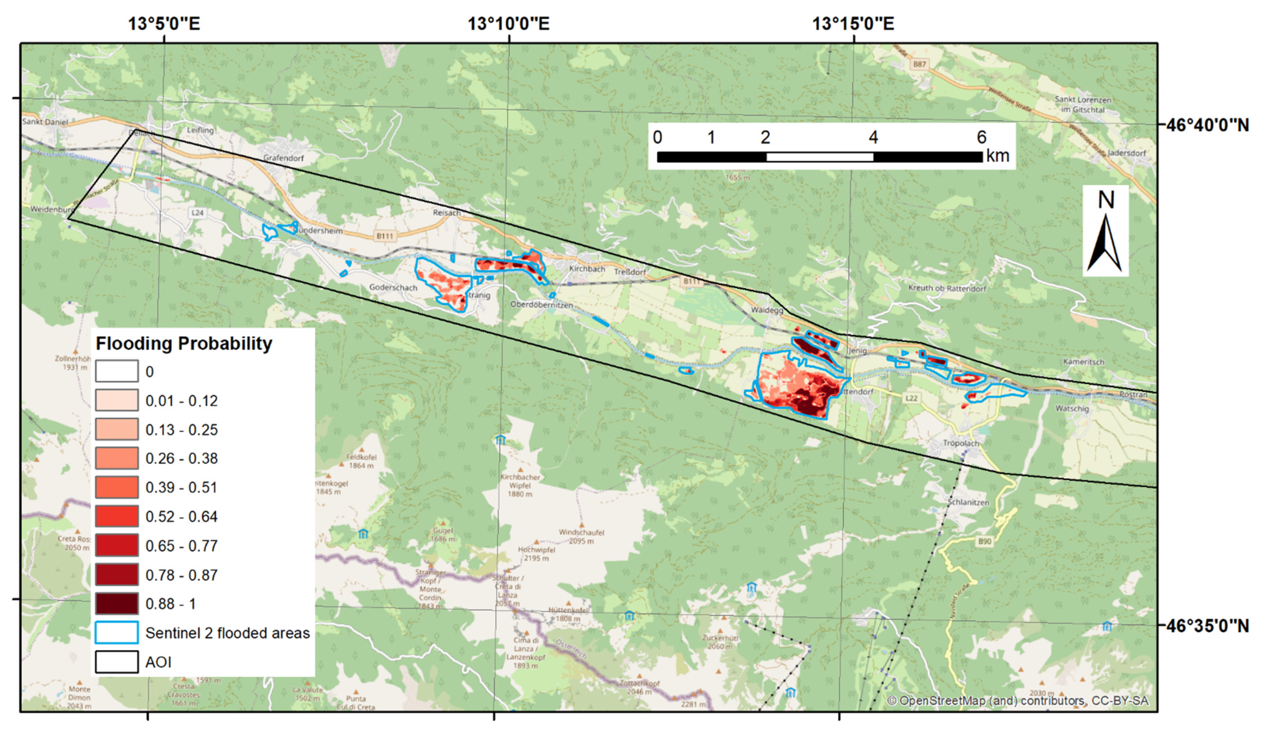
The map showing the extents of flooding from both sources is presented in Figure 8, while a statistical evaluation is found in

Table 2. Statistical evaluation of comparison between flood extent detected by developed solution and digitized from Sentinel-2 imagery for the Austria, 2018 flood event.

OA (%)	PA Open Water (%)	UA Open Water (%)	PA Other (%)	UA Other (%)	Kappa Coefficient
96.0	51.8	94.7	99.8	96.1	0.65

. The UA for open water reached 94.7 %, meaning that almost all pixels identified as flooded by the developed solution were also identified as flooded from the Sentinel-2 image. On the other hand, the PA for open water was only 51.8%, indicating that large areas identified as flooded from the Sentinel-2 image were not detected as flooded from the Sentinel-1 data processing. In this case, the reason for the situation can be at least partly found in the time of acquisition of used images. While Sentinel-2 images were acquired approximately 36 h after the water level culmination (see Figure 9), one Sentinel-1 image was available shortly after the beginning of water level rising and the second one was from approximately 72 h after the water level culmination. In that time, the extent of open water flooding was already significantly reduced.

4.3. The Czech Republic, Central Moravia, Spring 2020

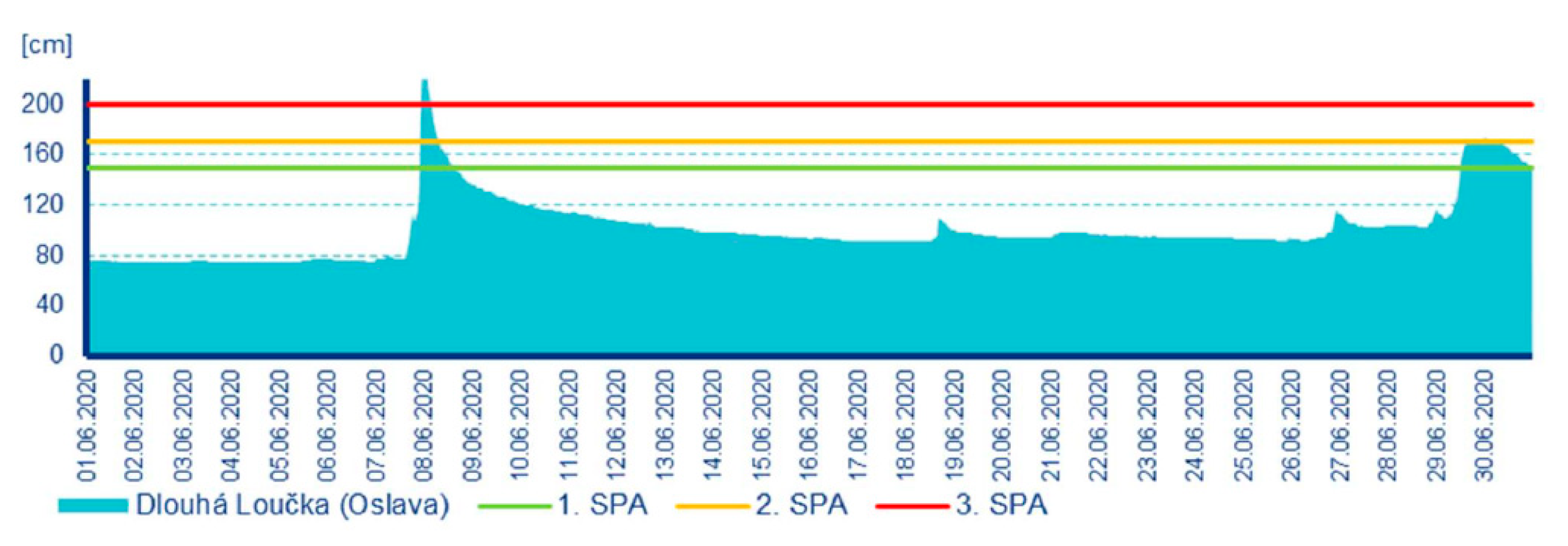
Severe torrential storms that hit the area north of Uničov city during the night from 7 June to 8 June 2020 resulted in a devastating flash flood. It caused the loss of life of two people and significant property damage (see, e.g., https://floodlist.com/europe/czech-republic-flash-floods-olomouc-june-2020, accessed on 1 September 2021). The officially reported level of flooding was equal to a 100-year return period. The course of flood event is provided in Figure 10, where the water level measured on the Oslava river at the hydrological station located in Dlouhá Loučka is plotted. In the first hours of June 8, a rapid increase of water level was visible, exceeding the third level of flooding activity (marked as SPA in the figure), which corresponds to a level of emergency. Shortly after culmination, the water level started to decrease. Due to the character of the flood event, the water passed quickly through the area and only several temporarily flooded lagoons were created, mostly on agricultural fields around lower parts of water streams in the selected AOI. Own photo documentation was acquired on June 8. The temporarily flooded lagoons disappeared quickly over the next several days.

For the validation of the developed flood detection solution, an area of 21 km² was selected. Data from the beginning of February until the end of August 2020 were processed from all four available tracks (A73, A175, D22, D124). In terms of false positives, three events were identified over the whole processed period. All of them occurred in track A175 during March and April. The extent of two of them are visualized in Figure 11.

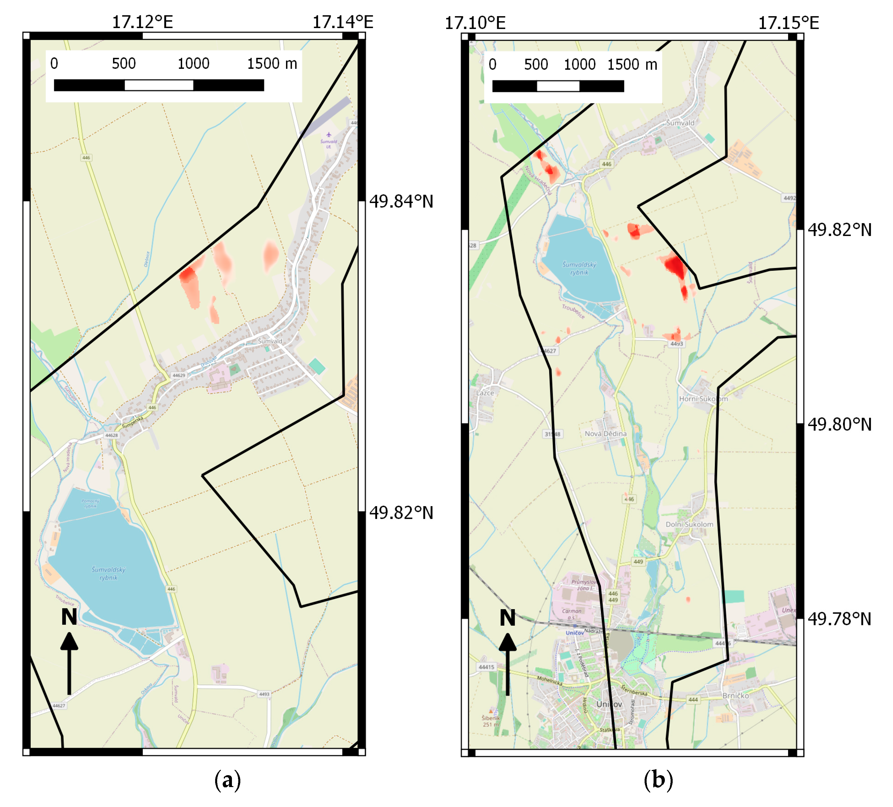
While it was not expected to detect the flooding in urban areas lying in the higher parts of water streams, some temporary water lagoons (see Figure 12) were supposed to be detected. Unfortunately, the flood was not detected in any track. Reasons leading to the failure in the detection of flooded lagoons were therefore analysed and are well understandable from the outputs provided in Figure 13, where the processing results of the Sentinel-1 image from track D124 acquired on 8 June 2020 are presented. Open water detection in both polarizations (VV, VH) provided correct results, as all four lagoons were detected as flooded. On the other hand, the lagoons were not detected by the change detection algorithm as areas where the backscatter intensity significantly changed compared to the state before the flood event. In this regard, an increased sensitivity of change detection in both polarizations was tested. When applied, lagoons n. 1, 2 and 4 were identified as changed in the VV polarization output, but none of them were identified as changed in the case of the VH output. Areas of all these four lagoons are agricultural fields where vegetation started to grow during the springtime, but a significant part of their surface was still bare soil when the flooding happened. Therefore, the change in backscatter intensity between this type of land cover and the flooded water was not high enough in VH to identify the area as changed, which prevented the overall flood detection.

Although taking only the outputs of the open water detection and neglecting the change detection results would bring good flood detection results in the described case, it cannot be applied generally, or at least not in the case of using the developed solution for autonomous flood monitoring. During validation, many situations were found when some area was wrongly detected as open water flooded, and only the negative result of change detection prevented the overall false positive. On the other hand, if the developed solution is run on demand for specific dates over an area where some flooding occurred, the outputs of open water detection themselves can be used for flood delineation if the change detection blocks the overall detection.

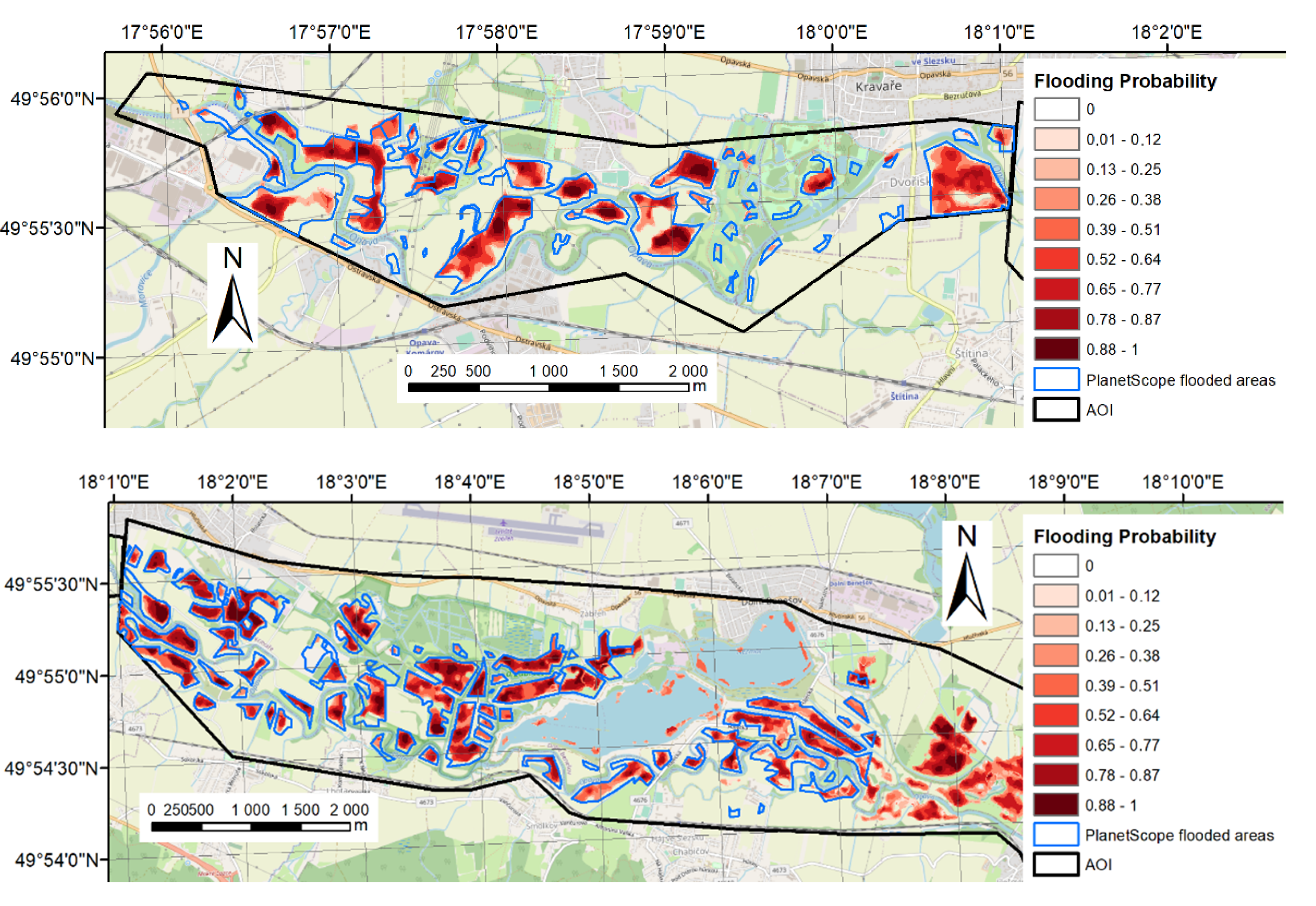
4.4. The Czech Republic, Northeastern Moravia, Autumn 2020

Regional floods hit several river basins in north-eastern and eastern Moravia during 14–16 October 2020 [33]. They were caused by continuous rainfalls starting on October 13 when previous rains had already saturated the soils. Although floods occurred in several territories, only two of them were selected for the validation because these were the only cases where reference optical imagery without strong cloud coverage was found. The selected two sub-areas are located east of Opava city, in the basin of the Opava river. The landscape is flat there, with prevailing meadows, agricultural fields, wetlands and various permanent water areas. The total surface area of both localities is 62 km².

Data from four Sentinel-1 tracks from the beginning of August to the middle of November, 2020 were processed for validation. No false positives occurred in the selected sub-areas during the processed period. For images acquired on October 14 (track A73) and 15 (track A175), floods were successfully detected in both sub-areas. In sub-area 2, floods with a much smaller extent were also detected from images collected on October 18 (track D124) and 19 (track D51). This was mainly due to the character of the selected sub-areas where sub-area 2 contains a complex of protected natural zones where flooding tends to remain longer and could be therefore detected from several consequent radar images.

A multispectral optical image acquired on 15 October 2020 by a PlanetScope satellite was used to create a reference data set. The eastern part of the image was entirely covered with cloudiness and was therefore excluded from the validation process. Figure 14 shows results from both sources, while

Table 3. Statistical evaluation of comparison between flood extent detected by the developed solution and digitized from a PlanetScope image for the Czech Republic, autumn 2020 flood event.

Sub-Area	OA (%)	PA Open Water (%)	UA Open Water (%)	PA Other (%)	UA Other (%)	Kappa Coefficient
1	89.2	63.3	92.0	98.1	88.5	0.68
2	92.2	73.1	92.1	98.1	92.2	0.77

contains their statistical comparison. Values of UA for the open water reached 92% in both sub-areas, while values of PA for the open water were 63% and 73%. Therefore, the situation was similar to the one described in previous sections, with a weaker flood detection from the developed solution compared to the reference data set.

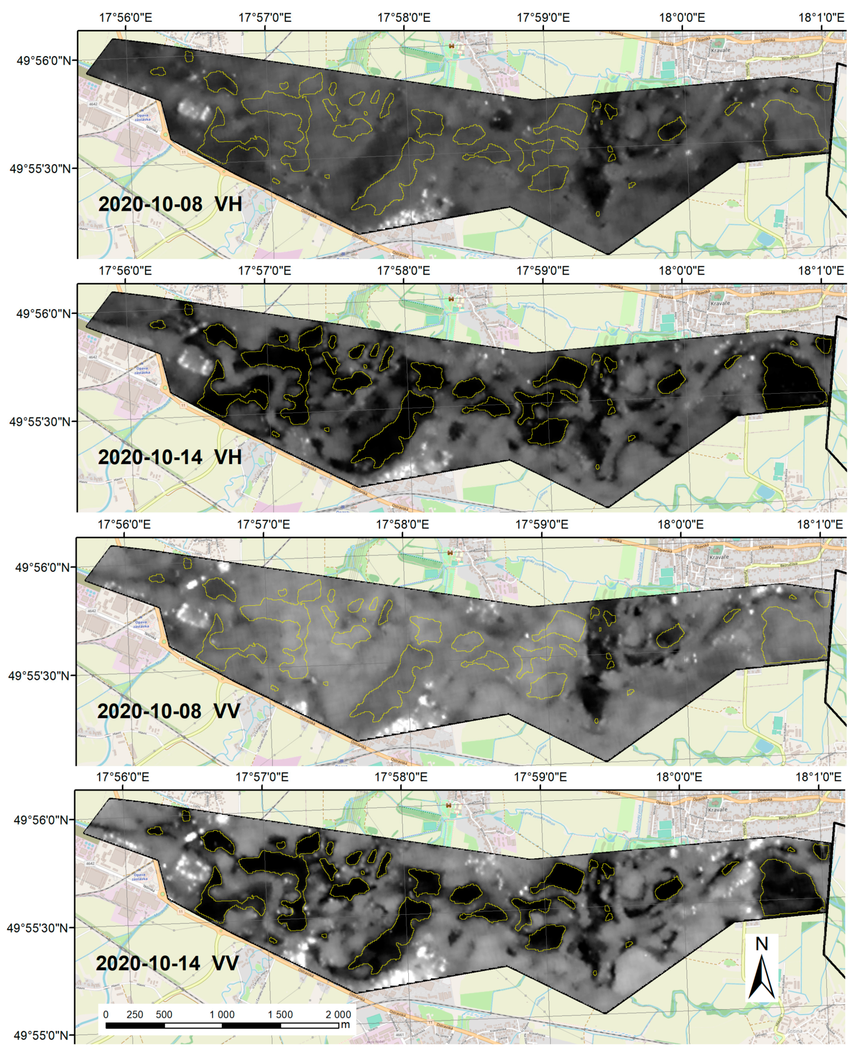
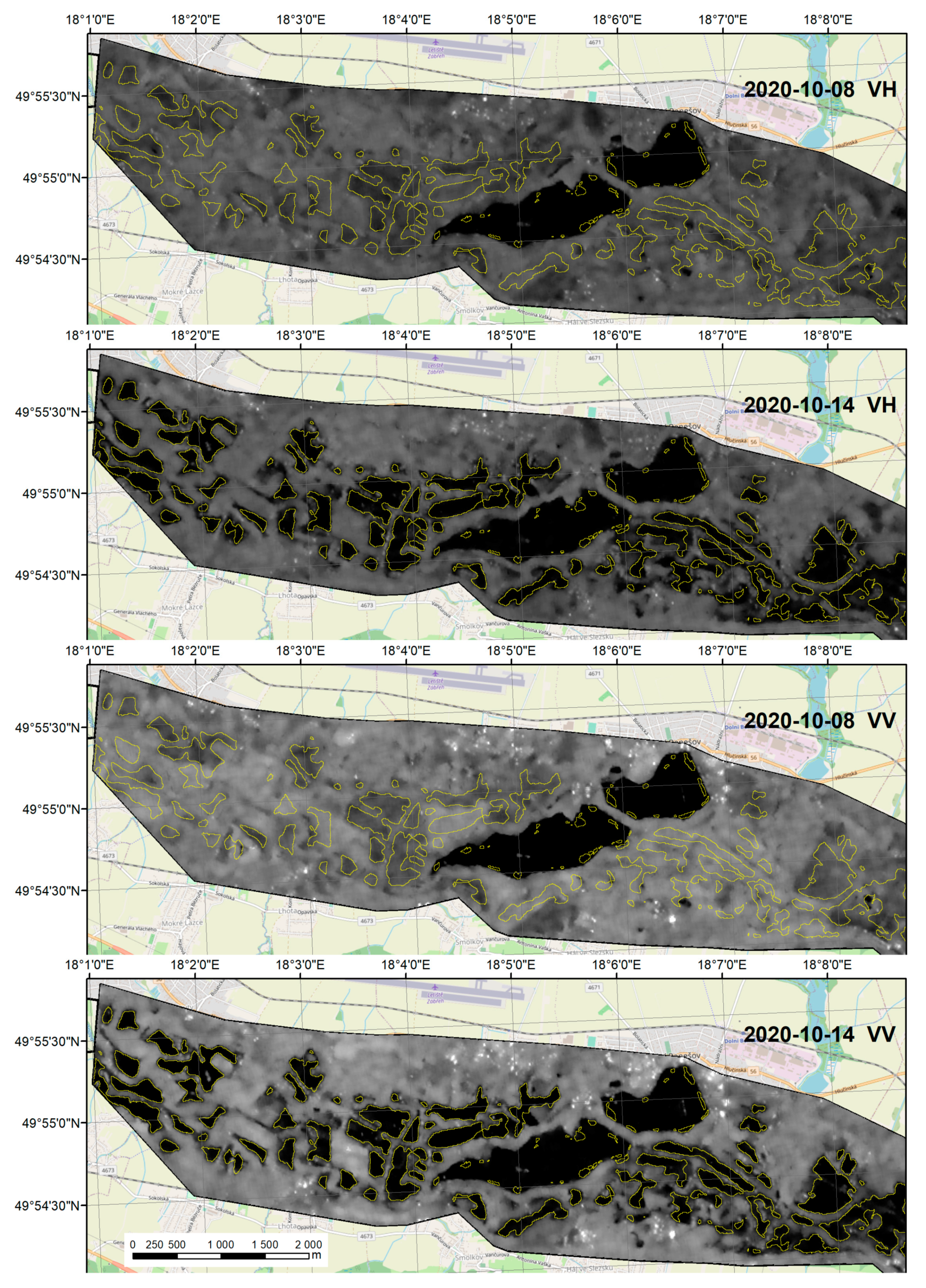
Figure 15 and Figure 16 provide the original Sentinel-1 imagery acquired over both processed sub-areas in track A73 on the day of flooding (14 October 2020) and several days before the flooding (8 October 2020). Dark areas in the images correspond to places with low backscatter intensity, typically represented by open water. The extent of flooding identified by the developed solution from the data acquired in this satellite track on 14 October 2020 are shown in yellow colour. It is well visible that most of dark-coloured areas in the Sentinel-1 imagery from 14 October 2020 were successfully identified as flooded by the developed solution.

4.5. Italy, Piedmont and Lombardy Regions, Autumn 2020

On 2–4 October 2020, extensive floods hit the Piedmont, Lombardy and Liguria regions. Storm Alex brought heavy rains reaching recording rainfalls; values exceeding 500 mm in 24 h were reported at some stations. For validation of the developed solution, a flood event at the river Sesia close to Vercelli city was selected, since it was also processed by the Copernicus Emergency Management Service (EMS), see https://emergency.copernicus.eu/mapping/list-of-components/EMSR468 (accessed on 31 August 2021). Two casualties and significant losses on the property were reported for this flood event.

Data from a single lowland area of 292 km² were processed, covering the period from the middle of September until the middle of October in three different Sentinel-1 tracks. Floods were successfully detected in the whole AOI from Sentinel-1 images acquired on October 3 (track A88) and October 4 (track A15). A few small polygons in the southern part of the processed area were also detected as flooded from the images acquired between October 8 and 15 (tracks D66, A15, A88). No false positives occurred during the processed period.

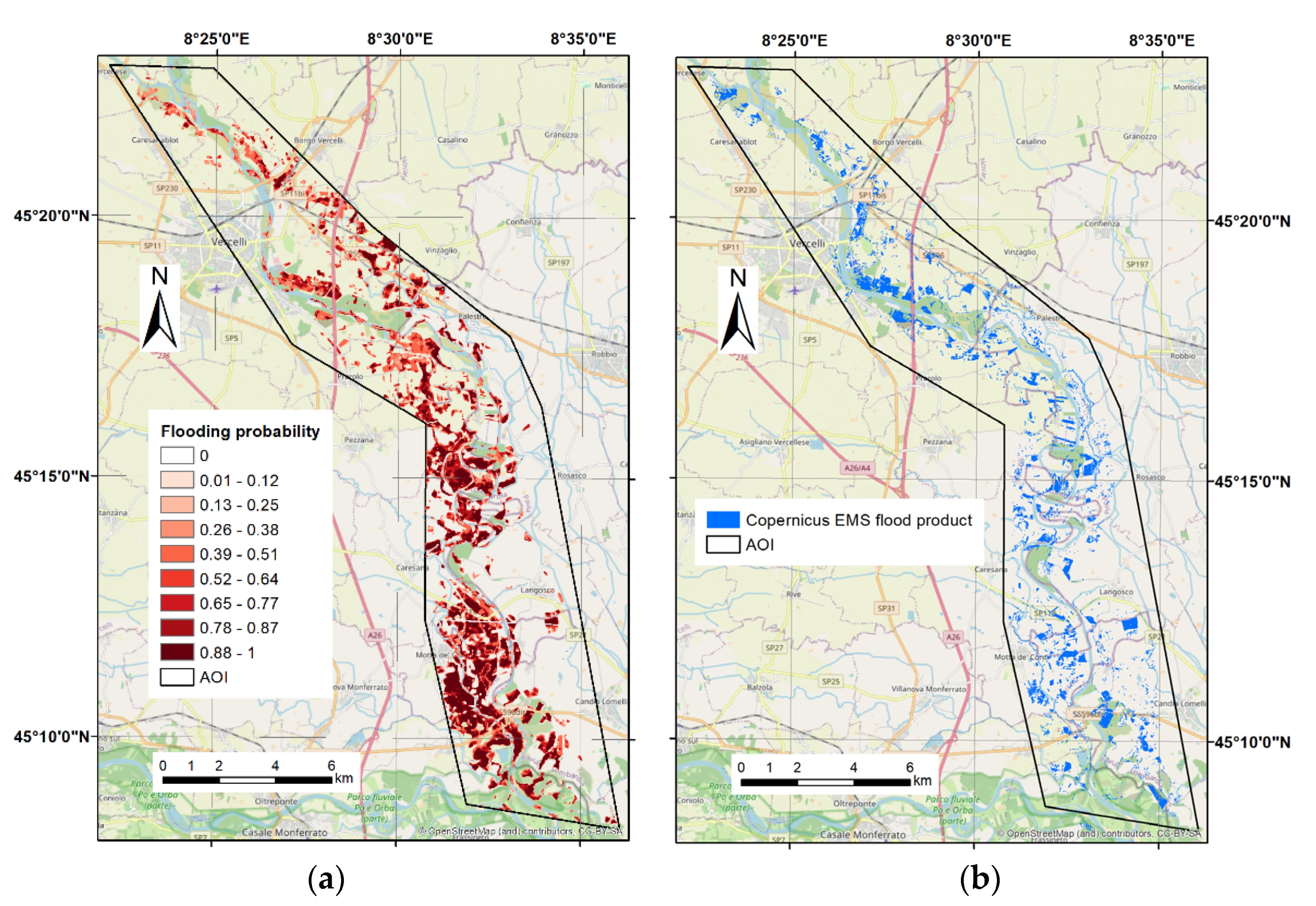
The extent of flood detection from the developed solution was compared with the flood delineation product provided by the Copernicus EMS. Its output was based on a RADARSAT image with a ground sample distance (GSD) of 3.0 m acquired on 6 October 2020 at 17:21 UTC. For a visual evaluation, maps showing the extent of flooding detected by the developed solution and Copernicus EMS are presented in Figure 17. Since the Sentinel-1 images used by the developed solution were acquired during the flood event while the RADARSAT image used by Copernicus EMS approximately three days after it, significantly larger areas were detected as flooded from the first source. Significantly more extensive flooding in the area than provided by the Copernicus EMS output are also visible in the Sentinel-2 image from October 3 (not shown).

On the other hand, the Copernicus EMS product also provided some flooded polygons in areas that were not detected as flooded by the developed solution. Usually, they were of small size and were therefore problematically detectable from Sentinel-1 imagery due to its coarser spatial resolution compared to RADARSAT. Still, a few larger polygons detected as flooded only by the Copernicus EMS product could be found, e.g., on urban surfaces close to Vercelli city or natural surfaces in the southern part of the processed area.

Table 4. Statistical evaluation of comparison between flood extent detected by the developed solution and the Copernicus EMS delineation product for the Italy, 2020 flood event.

OA (%)	PA Open Water (%)	UA Open Water (%)	PA Other (%)	UA Other (%)	Kappa Coefficient
76.5	45.5	15.2	79.1	94.6	0.13

contains the statistical evaluation of the comparison between the outputs of the developed solution and the Copernicus EMS. Values of PA and particularly of UA for open water were very low compared to results presented in previous sections for other flood events. This outcome can be attributed to reasons described in the previous paragraphs, mainly to the time difference in the acquisition of the Sentinel-1 and RADARSAT satellite images. That is why we do not include this locality in the summary of statistics provided in the Conclusion Section.

4.6. False Positives Testing in the South Moravia, 2019

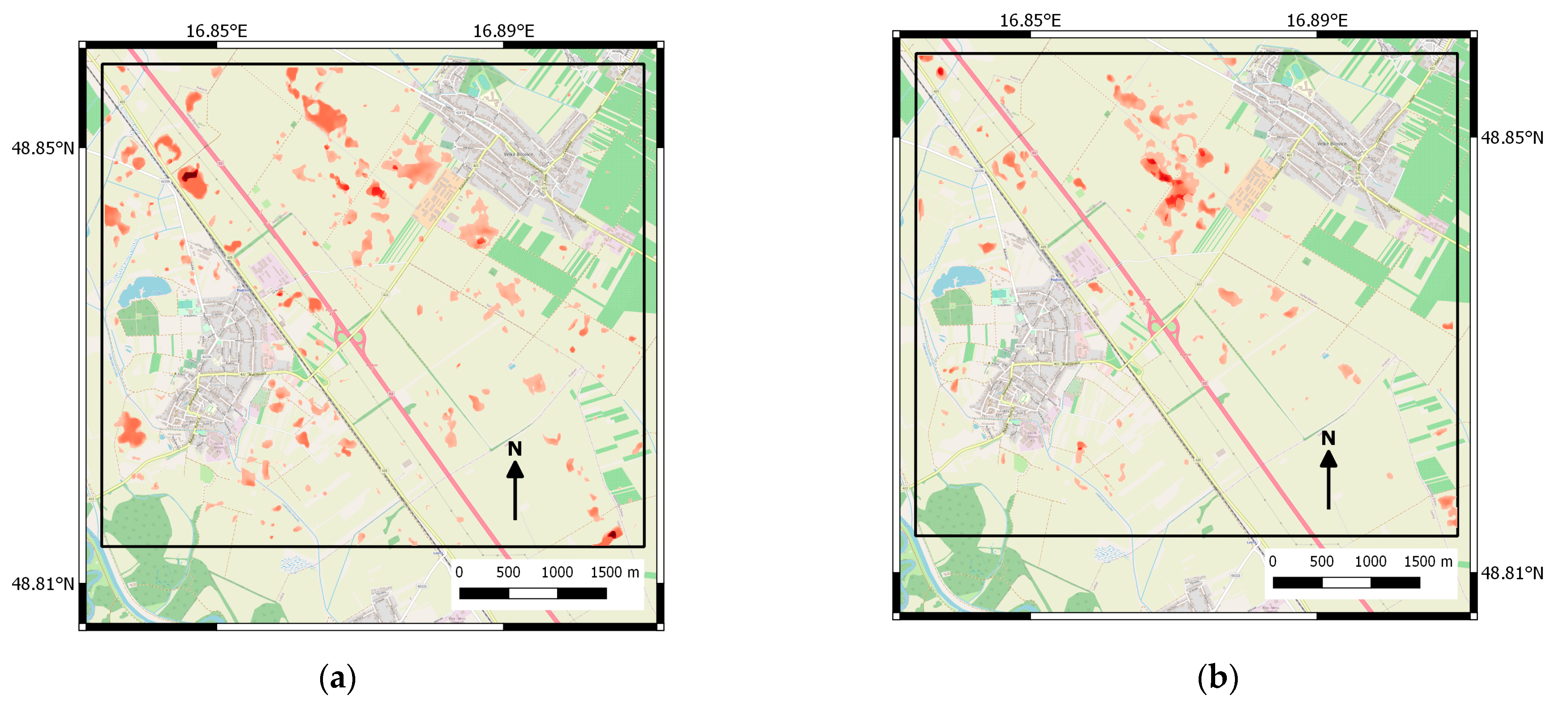
Data from a 27 km² rural locality in south Moravia were processed to thoroughly test the developed solution in terms of false positive occurrence. The selected area contains mainly extensively used agricultural fields and some urban areas or vineyards. Sentinel-1 images from three individual tracks spanning from the beginning of February until the end of December 2019 were tested. There were no false-positive alarms found in tracks D22 and D124. In track A73, three epochs with false-positive alarms occurred. All of them happened in April 2019; two of them are presented in the Figure 18. Since 55 epochs were processed for the A73 track, false positives occurred in 5.5% of epochs. Similar to the results presented in the previous sections, most areas wrongly detected as flooded were located on agricultural fields.

4.7. Flooding Detection from Individual Data Polarizations

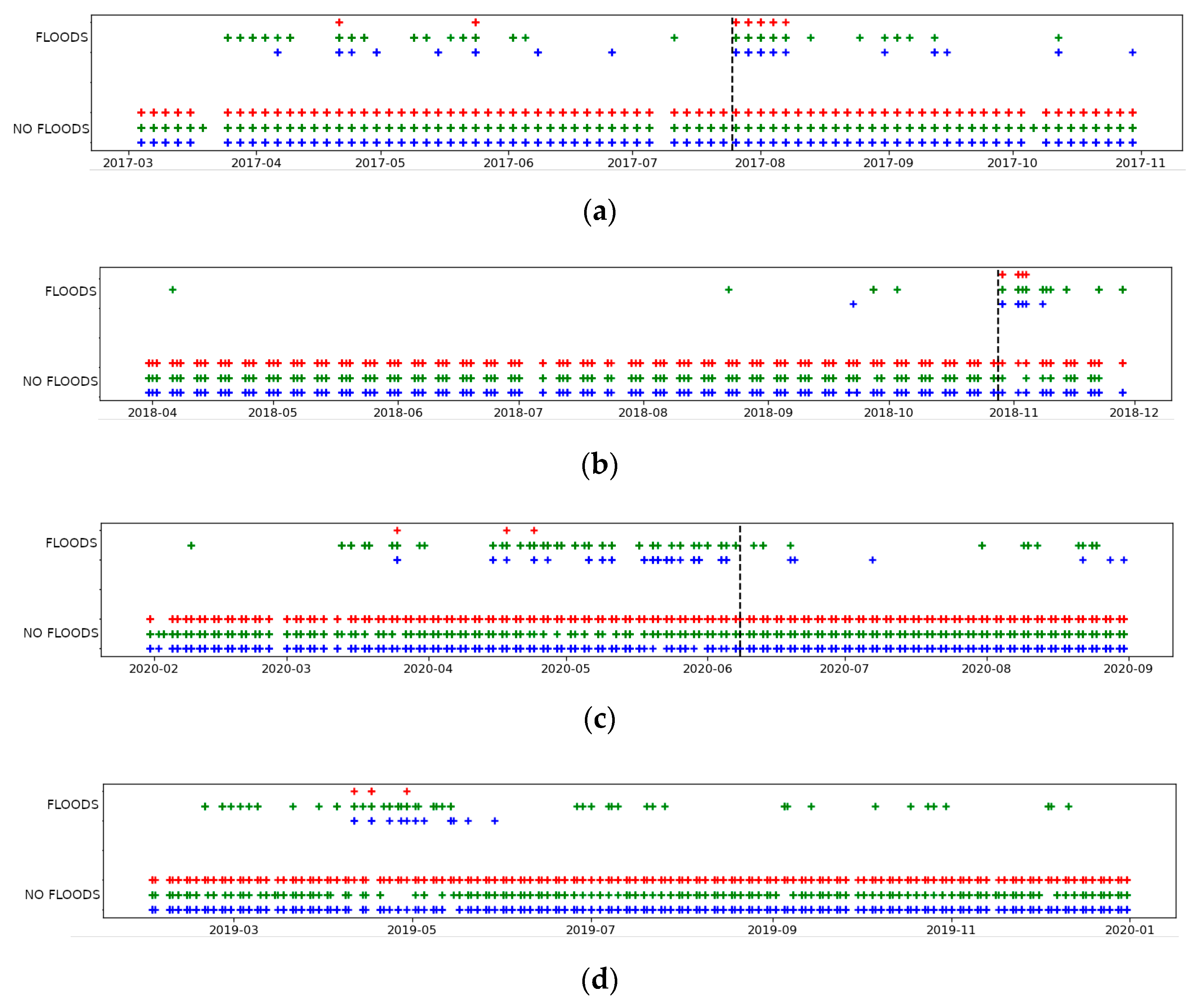
As mentioned in Section 3.1.4, the developed solution combines processing runs in both the VV and VH polarizations for a final result to suppress occurrence of false-positive detections. Figure 19 provides an overview of the frequency of false positive detections from processing based on individual polarizations and their combinations. From top to bottom, outputs for long-term processing over areas introduced in previous sections (Germany, Austria, central Moravia, south Moravia) are shown. It is evident that the number of final false-positives (red crosses in the upper row far away from the black line) is significantly lower than the number of false detections in either polarization (blue and green crosses in the upper row). In the VH polarization, a larger number of false-positive detections occurred compared to the VV polarization. The frequency of false-positive detections for the Austrian locality was much smaller compared to all three other localities. This is given by the prevailing land use. While the alpine valley in Austria consists mainly of meadows, the other three localities are intensively used for growing agricultural crops. Bare soils and various vegetation cover therefore change throughout the year, impacting the backscatter intensity of the radar signal, leading to false positives.

In Figure 19, there are several cases where the floods were detected in both polarizations, but not in their combination. It can be caused by two factors: (a) the floods were detected in another processed sub-area (Figure 19 displays aggregate results), or (b) more frequently, the floods were detected in the same sub-area, but on a different part of the sub-area. It is the most significant benefit of the use of both polarizations. In addition to the instances mentioned above, dates can be found where both the “FLOODS” and “NO FLOODS” states are present for a combination of both polarizations. This means that in some processed sub-areas, the flood was detected, but in some others, it was not.

5. Discussion

As confirmed by the validation, the developed solution can detect only open water pixels and only in non-urban areas due to Sentinel-1 resolution and SAR signal backscatter behaviour in the urban environment. In this regard, processing other SAR satellite data with the developed solution would be straightforward, except that with commercial data with a smaller coverage, it could be more difficult to find the needed permanent water bodies in the same image. We recommend using a permanent water bodies layer for the estimation of water–land thresholds. If the approach based on histogram bimodality is used instead, the reliability of the algorithm gets lower and can even lead to no detection of flooding in areas where the floods were correctly identified while using permanent water bodies in the input.

Generally, the quality of flood detection from SAR depends strongly on the acquisition time of the satellite images with respect to the flood culmination. As shown in Section 4.2 or Section 4.5, obtaining an image a few days after water culmination typically leads to a much weaker or even unsuccessful detection. A similar situation applies to flash floods, where the open water does not last long enough to be captured by the satellite. While using the developed solution, areas hit by a flash flood are often visible in the change-detection maps. However, without external information about flood occurrence in the area, they are not distinguishable from other changes such as those caused by common agricultural works. On the other hand, if the information on flood occurrence exists and the AOI covering potentially affected areas is provided, the method could be used in the on-demand mode while using only its change detection results for approximate delimitation of floods extent. A similar approach was described in [10] where a unique triggering mechanism was developed based on gauge stations and satellite precipitation estimations, identifying potentially flooded zones. Similarly, alerts issued by national meteorological services could be used.

Apart from the acquisition time of SAR imagery, differences between flood detection from the developed solution and reference data sets are supposed to be caused by two reasons.

Firstly, it can be caused by imperfections in open water manual identification from optical satellite imagery due to the varying quality of images and possibilities to mark large polygons as open water flooded, although some vegetation could have been above the water level, changing the radar’s reflection signal and limiting the detection.

Secondly, differences can be caused by weakening open water detection from the developed solution due to using universal parameter settings in automatic processing, as they were tuned to minimize the occurrence of false-positive detections.

In this regard, the results achieved by the developed solution can be compared to the results achieved by automatic SAR flood detectors presented by [2,3]. They both reported, for evaluated flood events, UAs for open water ranging from 82.4% to 99.3% and PAs for open water ranging from 83.6% to 98.5%. In [3], the kappa coefficient reached up to 0.91. While the UA for open water achieved by the developed solution typically exceeded 85%, The PA mostly was only between 60% and 70% and the maximum reached kappa coefficient was 0.77. On the other hand, [2,3] did not mention using automated flood detection solutions to process data over a long-term period to evaluate potential false positives. They focused only on the selected flood events themselves. Other authors, such as [10], do not operate their system permanently, but only in areas and at times when their triggering mechanism reported potential floods. We consider the presented long-term tests to be an essential part of the quality assessment of our developed solution.

The above-mentioned search for universal parameters was necessary as the developed solution is supposed to be run primarily as an automatic continuous monitoring over an area of client’s interest and not on-demand over areas with already proven flooding. As found by performing a set of tests, increasing flood detection sensitivity led to an increasing extent of flood detection, but also to an increasing number of false positives. Increased sensitivity is mainly valid for the change detection algorithm where a statistically significant change in backscatter intensity must happen between the pre-event stack of images and the image evaluated for flooding to allow for flood detection.

6. Conclusions

In this work, we presented a developed automatic flood detection solution based on Sentinel-1 multi-temporal imagery. Although it can be run in on-demand mode, it was prepared mainly for autonomous continuous monitoring of potential flooding in a given area. The solution combines change detection and open-water detection algorithms; both run in the VH and VV polarizations. The only auxiliary data which should be provided by the user are a layer defining AOI and a layer defining permanent water bodies within or near the AOI.

The results of validating the developed solution on five flood events in Europe and an additional false positive test in a rural landscape were provided. Data from long-term periods were processed for at least two satellite tracks and the delivered outputs were compared with prepared reference datasets based on optical or SAR imagery. Floods were successfully detected in four riverine flood events; the method failed in the case of the flash flood event. The classification metrics were computed to statistically compare the extent of floods identified from the developed solution and the reference datasets. The overall accuracy values mostly exceeded 95%. With an exception for the Italian flood event, user accuracy values for the open-water class ranged between 55% and 95%, with a mean of 83%. A high percentage of pixels identified as flooded by the developed solution were also flooded according to the used reference dataset. On the other hand, producer accuracy values for the open-water class were on average only 65%. The developed solution usually provided flooded polygons of a smaller size or did not detect a flood in some places where the reference dataset did. This influenced kappa coefficient values which ranged between 0.59 and 0.77. According to [34], values between 0.61 and 0.80 correspond a substantial level of agreement. Except for the quality of the prepared reference datasets (influenced by differences in real flooding extent happening between times of acquisition of the Sentinel-1 and reference dataset imagery and imperfections during the manual digitization of reference imagery) the described situation is mainly attributed to the applied tuning of sensitivity parameters to limit false positives. Increasing the sensitivity of flood detection leads to increased flood detection, but also to a higher number of false positives. The flash flood at the beginning of June, 2020 near Uničov city in the Czech Republic was not detected with the developed solution since temporarily flooded water lagoons at agricultural fields were not identified with the change detection algorithm to differ significantly from their pre-event state.

Zero or minimum false positives occurred in all processed events and included sub-areas with various land cover and land use characteristics. All of the false positives were identified during the spring season (from late March till the end of May) and the majority of areas wrongly detected as flooded lay at agricultural land. Therefore, the origin of the false positives is related to changes in agricultural fields during the beginning of the vegetation season and at times of crop harvesting or extensive agricultural work. The developed solution currently does not use any auxiliary data to suppress false positives. In this regard, implementing, e.g., the topo-hydrological factor HAND (height above nearest drainage, [35]), which is also used in SAR-based flood detection solutions by [3] or [5], could be helpful.

References

1. Martinis, S.; Twele, A.; Voigt, S. Towards operational near-real time flood detection using a split-based automatic thresholding procedure on high resolution TerraSAR-X data. Nat. Hazards Earth Syst. Sci. 2009, 9, 303–314. [Google Scholar] [CrossRef]
2. Martinis, S.; Kersten, J.; Twele, A. A fully automated TerraSAR-X based flood service. ISPRS J. Photogramm. Remote Sens. 2015, 104, 203–212. [Google Scholar] [CrossRef]
3. Twele, A.; Cao, W.; Plank, S.; Martinis, S. Sentinel-1-based flood mapping: A fully automated processing chain. Int. J. Remote Sens. 2016, 37, 2990–3004. [Google Scholar] [CrossRef]
4. Pulvirenti, L.; Pierdicca, N.; Chini, M.; Guerriero, L. An algorithm for operational flood mapping from Synthetic Aperture Radar (SAR) data based on the fuzzy logic. Nat. Hazards Earth Syst. Sci. 2011, 11, 529–540. [Google Scholar] [CrossRef] [Green Version]
5. Bioresita, F.; Puissant, A.; Stumpf, A.; Malet, J.-F. A Method for Automatic and Rapid Mapping of Water Surfaces from Sentinel-1 Imagery. Remote Sens. 2018, 10, 217. [Google Scholar] [CrossRef] [Green Version]
6. Moharrami, M.; Javanbakht, M.; Attarchi, S. Automatic flood detection using sentinel-1 images on the google earth engine. Environ. Monit. Assess. 2021, 193, 278. [Google Scholar] [CrossRef]
7. Alexandre, C.; Johary, R.; Catry, T.; Mouquet, P.; Révillion, C.; Rakotondraompiana, S.; Pennober, G. A Sentinel-1 Based Processing Chain for Detection of Cyclonic Flood Impacts. Remote Sens. 2020, 12, 252. [Google Scholar] [CrossRef] [Green Version]
8. de la Cruz, R.M.; Olfindo, N.T.; Felicen, N.N., Jr.; Borlongan, N.J.B.; Difuntorum, J.K.L.; Marciano, J.J.S., Jr. Near-real Time Flood Detection from Multi-Temporal Sentinel Radar Images using Artificial Intelligence. The International Archives of the Photogrammetry, Remote Sensing and Spatial Information Sciences, Volume XLIII-B3-2020, 2020 XXIV ISPRS Congress. 2020. Available online: https://www.int-arch-photogramm-remote-sens-spatial-inf-sci.net/XLIII-B3-2020/1663/2020/isprs-archives-XLIII-B3-2020-1663-2020.pdf (accessed on 29 November 2021).
9. Nallapareddy, A.; Balakrishnan, B. Automatic Flood Detection in Multi-Temporal Sentinel-1 Synthetic Aperture Radar Imagery Using ANN Algorithms. Int. J. Comput. Commun. Control 2020, 15, 3. [Google Scholar] [CrossRef] [Green Version]
10. Yang, Q.; Shen, X.; Anagnostou, E.N.; Mo, C.; Eggleston, J.R.; Kettner, A.J. A High-Resolution Flood Inundation Archive (2016–the Present) from Sentinel-1 SAR Imagery over CONUS. Bull. Am. Meteorol. Soc. 2021, 102, E1064–E1079. [Google Scholar] [CrossRef]
11. Mohammadi, A.; Kamran, K.V.; Karimzadeh, S.; Shahabi, H.; Al-Ansari, N.; Selişteanu, D. Flood Detection and Susceptibility Mapping Using Sentinel-1 Time Series, Alternating Decision Trees, and Bag-ADTree Models. Complexity 2020, 2020, 4271376. [Google Scholar] [CrossRef]
12. Mason, D.C.; Speck, R.; Devereux, B.; Schumann, G.J.-P.; Neal, J.C.; Bates, P.D. Flood detection in urban areas using TerraSAR-X. IEEE. Trans. Geosci. Remote Sens. 2010, 48, 882–894. [Google Scholar] [CrossRef] [Green Version]
13. Mason, D.C.; Dance, S.L.; Vetra-Carvalho, S.; Cloke, H.L. Robust algorithm for detecting floodwater in urban areas using synthetic aperture radar images. J. Appl. Remote Sens. 2018, 12, 045011. [Google Scholar] [CrossRef] [Green Version]
14. Mason, D.C.; Bevington, J.; Dance, S.; Revilla-Romero, B.; Smith, R.; Vetra-Carvalho, S.; Cloke, H. Improving Urban Flood Mapping by Merging Synthetic Aperture Radar-Derived Flood Footprints with Flood Hazard Maps. Water 2021, 13, 1577. [Google Scholar] [CrossRef]
15. Giustarini, L.; Hostache, R.; Matgen, P.; Schumann, G.J.; Bates, P.D.; Mason, D.C. A Change Detection Approach to Flood Mapping in Urban Areas Using TerraSAR-X. IEEE Trans. Geosci. Remote Sens. 2013, 51, 2417–2430. [Google Scholar] [CrossRef] [Green Version]
16. Chini, M.; Pelich, R.; Pulvirenti, L.; Pierdicca, N.; Hostache, R.; Matgen, P. Sentinel-1 InSAR Coherence to Detect Floodwater in Urban Areas: Houston and Hurricane Harvey as A Test Case. Remote Sens. 2019, 11, 107. [Google Scholar] [CrossRef] [Green Version]
17. Jo, M.; Osmanoglu, B. Generating Flood Probability Map Based on Combined Use of Synthetic Aperture Radar and Optical Imagery. In Proceedings of the IGARSS 2020–2020 IEEE International Geoscience and Remote Sensing Symposium, Virtual, 26 September–2 October 2020. [Google Scholar]
18. Mason, D.C.; Dance, S.L.; Cloke, H.L. Floodwater detection in urban areas using Sentinel-1 and WorldDEM data. J. Appl. Remote Sens. 2021, 15, 032003. [Google Scholar] [CrossRef]
19. Pierdicca, N.; Pulvirentia, L.; Chini, M.; Guerrieroc, L.; Candelad, L. Observing floods from space: Experience gained from COSMO-SkyMed observations. Acta Astronaut. 2013, 84, 122–133. [Google Scholar] [CrossRef]
20. Pulvirenti, L.; Pierdicca, N.; Chini, M.; Guerriero, L. Monitoring Flood Evolution in Vegetated Areas Using COSMO-SkyMed Data: The Tuscany 2009 Case Study. IEEE J. Sel. Top. Appl. Earth Obs. Remote Sens. 2013, 6, 1807–1816. [Google Scholar] [CrossRef]
21. Plank, S.; Jussi, M.; Martinis, S.; Twele, A. Mapping of flooded vegetation by means of polarimetric Sentinel-1 and ALOS-/PALSAR-2 imagery. Int. J. Remote Sens. 2017, 38, 3831–3850. [Google Scholar] [CrossRef]
22. Tsyganskaya, V.; Martinis, S.; Marzahn, P.; Ludwig, R. Detection of Temporary Flooded Vegetation Using Sentinel-1 Time Series Data. Remote Sens. 2018, 10, 1286. [Google Scholar] [CrossRef] [Green Version]
23. DeVries, B.; Huang, C.; Armston, J.; Huang, W.; Jones, J.W.; Lang, M.W. Rapid and robust monitoring of flood events using Sentinel-1 and Landsat data on the Google Earth Engine. Remote Sens. Environ. 2020, 240, 111664. [Google Scholar] [CrossRef]
24. Papila, I.; Alganci, U.; Sertel, E. Sentinel-1 Based Flood Mapping Using Interferometric Coherence and Intensity Change Detection Approach. Int. Arch. Photogramm. Remote Sens. Spat. Inf. Sci. 2020, 43, 1697–1703. [Google Scholar] [CrossRef]
25. Zhang, M.; Chen, F.; Liang, D.; Tian, B.; Yang, A. Use of Sentinel-1 GRD SAR Images to Delineate Flood Extent in Pakistan. Sustainability 2020, 12, 5784. [Google Scholar] [CrossRef]
26. Reksten, J.H.; Salberg, A.-B.; Solberg, R. Flood Detection in Norway Based on Sentinel-1 SAR Imagery. Int. Arch. Photogramm. Remote Sens. Spat. Inf. Sci. 2019, XLII-3/W8, 349–355. [Google Scholar] [CrossRef] [Green Version]
27. Shen, X.; Wang, D.; Mao, K.; Anagnostou, E.; Hong, Y. Inundation Extent Mapping by Synthetic Aperture Radar: A Review. Remote Sens. 2019, 11, 879. [Google Scholar] [CrossRef] [Green Version]
28. Clement, M.A.; Kilsby, C.G.; Moore, P. Multi-temporal synthetic aperture radar flood mapping using change detection. J. Flood Risk Manag. 2017, 11, 152–168. [Google Scholar] [CrossRef]
29. Lee, J.S.; Wen, J.H.; Ainsworth, T.L.; Chen, K.S.; Chen, A. Improved Sigma filter for speckle filtering of SAR imagery. IEEE Trans. Geosci. Remote Sens. 2009, 47, 202–213. [Google Scholar] [CrossRef]
30. Anhalt, M.; Bindick, S.; Meyer, S. Das Juli-Hochwasser 2017 im Südlichen Niedersachsen. Niedersächsischer Landesbetrieb für Wasserwirtschaft, Küsten- und Naturschutz. 2017. Available online: https://www.nlwkn.niedersachsen.de/download/124949 (accessed on 8 April 2021).
31. Moser, J.; Kopeinig, C.; Gutschi, E.; Malle, H.; Koboltschnig, G.; Schober, S.; Kulterer, K.; Schabus, V. Hofer: Hochwasserereignis an der Drau, Möll, Gail und Zubringern 28–31.10.2018. Hydrologischer Bericht (Endbericht). 2019. Available online: https://www.ktn.gv.at/Themen-AZ/Details?thema=11&subthema=58&detail=383 (accessed on 8 April 2021).
32. Čekal, R.; Šrámek, J.; Gvoždíková, B.; Handžák, Š.; Rosa, J.; Sandev, M.; Šopko, F.; Šustková, V.; Volný, R.; Crhová, L.; et al. Povodně na území České Republiky v Červnu 2020. Czech Hydrometeorological Institute. 2020. Available online: https://www.chmi.cz/files/portal/docs/poboc/CB/pruvodce/povodnove_zpravy/cr_2020_06.pdf (accessed on 8 May 2021).
33. Čekal, R.; Šrámek, J.; Dvořák, M.; Sýkorová, P.; Crhová, L.; Boráková, J.; Černá, I.; Hančarová, E.; Kamínková, A.; Macháčková, H.; et al. Povodně na Území České Republiky v Říjnu 2020. Czech Hydrometeorological Institute. 2020. Available online: https://www.chmi.cz/files/portal/docs/poboc/CB/pruvodce/povodnove_zpravy/cr_2020_10.pdf (accessed on 8 May 2021).
34. Landis, R.; Koch, G. The Measurement of Observer Agreement for Categorical Data. Biometrics 1977, 33, 159–174. [Google Scholar] [CrossRef] [Green Version]
35. Nobre, A.D.; Cuartas, L.A.; Hodnett, M.; Rennó, C.D.; Rodrigues, G.; Silveira, A.; Waterloo, M.; Saleska, S. Height above the Nearest Drainage—A hydrologically relevant new terrain model. J. Hydrol. 2011, 404, 13–29. [Google Scholar] [CrossRef] [Green Version]
Figure 1. Flowchart of the designed flood detection processing chain. Blue colour text represents inputs; magenta colour text represents outputs (i.e., maps and output states (in uppercase)). Black rectangles indicate processing steps, while green rectangles indicate decisions (with red colour indicating possible choices).
Water 13 03392 g001
Figure 2. Examples of the “Z” (a) and “SS” (b) fuzzy functions. The “Z” function is applied within open-water detection (input value is the SAR intensity, thresholds t1 and t2 are estimated from data), the “SS” function is applied on the change detection results (input is the change detection statistics: difference divided by the statistically critical difference, thresholds t1 and t2 are pre-set). The “SS” function allows the preservation of the sign of the change.
Water 13 03392 g002
Figure 3. Determination of the water–land threshold based on a bimodal histogram (a) and a permanent water histogram (b).
Water 13 03392 g003
Figure 4. Water–land threshold estimation and adaptation for the bimodal histogram method (a) and the open-water histogram method (b). The red lines indicate the thresholds t1, t2, estimated from the histogram, while the solid green line indicates the extended t2 threshold. The dashed green line indicates the maximum allowed threshold t2 (hard limit).
Water 13 03392 g004
Figure 5. Individual sub-areas selected to validate the flood event close to Hannover in Germany, 2017. Source of background map: Open Street Map (OSM).
Water 13 03392 g005
Figure 6. False-positive flood detection in part of sub-area 2 from Sentinel-1 images in track A117 acquired on 24 May 2017. Flooded areas are shown in red. Source of background map: Open Street Map (OSM).
Water 13 03392 g006
Figure 7. Flood extent detected by the developed solution (in red) from Sentinel-1 images acquired on July 29 and on 1 August, 2017. Manually digitized flood extent (in blue) from Sentinel-2 imagery acquired on 31 July 2017. (a) The southern part of sub-area 1 and (b) sub-area 7 in Germany, 2017.
Water 13 03392 g007
Figure 8. Flood extent detected by the developed solution (in red) from Sentinel-1 images acquired on 29 October and on 2 November, 2018. Manually digitized flood extent (in blue) from a Sentinel-2 image acquired on 31 November 2018. The western part of the area selected for the flood event in Austria, 2018. Source of background map: Open Street Map (OSM).
Water 13 03392 g008
Figure 9. The water level at the Rattendorf hydrological station on river Gail from 28–31 October 2018. Black lines show the times of Sentinel-1 and Sentinel-2 image acquisition. Source of original image: [31].
Water 13 03392 g009
Figure 10. The water level at Dlouhá Loučka station on the river Oslava during June 2020. SPA corresponds to level of flooding activity. Source: [32].
Water 13 03392 g010
Figure 11. False-positive flood detection in parts of the processed area for the Uničov flood event from Sentinel-1 images in track A175 from (a) March 25 and (b) April 18, 2020. Flooded areas are shown in red using the same colour scale as in Figure 9. The Borderline of the AOI is shown in black.
Water 13 03392 g011
Figure 12. Photo documentation of four temporary lagoons near Uničov city from 8 June 2020. The location of each lagoon is shown in Figure 13, and given by its number.
Water 13 03392 g012
Figure 13. Flood detection from Sentinel-1 images from track D124 acquired on June 8, 2020. Results of open water detection in VV polarization (a) and VH polarization (b), results of change detection in VV (c) and VH (d). For open water, the darker the red colour, the higher the probability of open water presence. For change detection, the blue (red) colour represents a statistically significant increase (decrease) of backscatter intensity compared to the pre-event situation. Numbers in (a) depict the locations of the temporary water lagoons shown in Figure 12.
Water 13 03392 g013
Figure 14. Flood extent detected by the developed solution (in red) from Sentinel-1 images acquired on 14 October and 15 October 2020. Manually digitized flood extent (in blue) from a Planet Scope image acquired on 15 November 2020. Sub-area 1 (top) and sub-area 2 (bottom) in the Czech Republic, autumn 2020. Source of background map: Open Street Map (OSM).
Water 13 03392 g014
Figure 15. Sentinel-1 imagery from track A73 acquired during the flood event (14 October 2020) and before the flood event (8 October 2020) in sub-area 1 (see Figure 14). Dates of image acquisition and data polarization is printed in each figure. The symbology is different for different data polarizations, black corresponds to −26/−20 dB (VH/VV) or lower, and white colour corresponds to +2/+1 dB (VH/VV) or higher. Areas identified as flooded by the developed solution from the Sentinel-1 data for 14 October 2020 are shown in yellow in all the figures. Source of background map: Open Street Map (OSM).
Water 13 03392 g015
Figure 16. Sentinel-1 imagery from track A73 acquired during the flood event (14 October 2020) and before the flood event (8 October 2020) in the sub-area 2 (see Figure 14). Dates of image acquisition and data polarization are printed in each figure. The symbology is different for different data polarizations, black colour corresponds to −26/−20 dB (VH/VV) or lower and white colour corresponds to +2/+1 dB (VH/VV) or higher. Areas identified as flooded by the developed solution from the Sentinel-1 data of 14 October 2020 are shown in yellow in all figures. Source of background map: Open Street Map (OSM).
Water 13 03392 g016
Figure 17. (a) Flood extent detected by the developed solution (in red) from Sentinel-1 images acquired on October 3 and on 4 October 2020. (b) Flood product from the Copernicus EMS (in blue) based on a RADARSAT image acquired on 6 October 2020. River Sesia in Italy, autumn 2020. Source of background map: Open Street Map (OSM).
Water 13 03392 g017
Figure 18. False-positive flood detection in south Moravia from Sentinel-1 images in track A73 from (a) 11 April and (b) 29 April 2019. Flooded areas are shown in red using the same colour scale as in previous figures. Source of background map: Open Street Map (OSM).
Water 13 03392 g018
Figure 19. Frequency of false positives for various processed localities: (a) Germany, (b) Austria, (c) central Moravia, (d) south Moravia. The black dashed line indicates the date of the start of the real flood event (no floods in south Moravia). Blue crosses represent VV polarization; green crosses represent VH polarization; red crosses represent their combination (final result). The crosses are plotted for all processed tracks and all processed sub-areas.
Water 13 03392 g019