
The Applications of Soft Computing Methods for Seepage Modeling: A Review


1
Institute of Geographic Sciences and Natural Resources Research, The Chinese Academy of Sciences, Beijing 100101, China
2
Center of Excellence in Hydroinformatics and Faculty of Civil Engineering, University of Tabriz, 29 Bahman Ave., Tabriz 5166616471, Iran
3
Faculty of Natural Sciences, University of Silesia in Katowice, 60 Będzińska Str., 41-200 Sosnowiec, Poland
*
Author to whom correspondence should be addressed.
Water 2021, 13(23), 3384; https://doi.org/10.3390/w13233384
Submission received: 13 August 2021
/
Revised: 27 October 2021
/
Accepted: 25 November 2021
/
Published: 1 December 2021
(This article belongs to the Special Issue Application of Data Pre-post Processing Methods for Modeling Hydro-Climatologic Processes)
Abstract
:In recent times, significant research has been carried out into developing and applying soft computing techniques for modeling hydro-climatic processes such as seepage modeling. It is necessary to properly model seepage, which creates groundwater sources, to ensure adequate management of scarce water resources. On the other hand, excessive seepage can threaten the stability of earthfill dams and infrastructures. Furthermore, it could result in severe soil erosion and consequently cause environmental damage. Considering the complex and nonlinear nature of the seepage process, employing soft computing techniques, especially applying pre-post processing techniques as hybrid methods, such as wavelet analysis, could be appropriate to enhance modeling efficiency. This review paper summarizes standard soft computing techniques and reviews their seepage modeling and simulation applications in the last two decades. Accordingly, 48 research papers from 2002 to 2021 were reviewed. According to the reviewed papers, it could be understood that regardless of some limitations, soft computing techniques could simulate the seepage successfully either through groundwater or earthfill dam and hydraulic structures. Moreover, some suggestions for future research are presented. This review was conducted employing preferred reporting items for systematic reviews and meta-analyses (PRISMA) method.
1. Introduction
More than two billion of the world’s population depends on groundwater resources, and about half of the irrigation water used to grow the world’s food comes from groundwater. Moreover, groundwater can be considered a vital resource in times of drought. Economic and population increases around the world are moving groundwater into the headlines. In developing countries, groundwater shortage and contamination excessively influence the destitute since they cannot regularly keep up with sinking groundwater levels or discover elective sources when their groundwater asset is contaminated. Moreover, in industrialized nations, the economic livelihood of the whole locales is affected by groundwater [1]. Numerous regions worldwide are subject to overexploitation of groundwater, experiencing water deficiencies because of a discrepancy between water supply and request. Additionally, it is well known that the request for groundwater will increase considerably over time due to the developing populace and financial advancement [2]. Even though climatic factors primarily control water supply, the administration and the resulting practices altogether influence the accessibility of water. Within the case of groundwater sources, unsuitable management could result in declining water sources; however, additionally, it leads to a reduction in the quality of groundwater [3]. Considering the importance of groundwater, the most dominant factor in the investigation and study of groundwater is water seepage, which explores and analyzes the issue of water movement in the porous media.
Moreover, the construction and use of earthfill dams and structures to solve the water shortage is essential, although this solution alone is not enough to overcome this problem. Earthfill dams are the foremost common sorts of the dam. Furthermore, they may be taken into consideration as the foremost choice when employing regionally accessible materials. Additionally, they have been a part of a normal procedure to store and control stream water for a long time. Stability and seepage are vital in an earthfill dam as they were found to be the significant reasons for dam failure. In order to prevent dam failure, it is essential to control the seepage in the dam. Seepage in dams causes water waste and the decline of dam stability. Earthfill dams lose water in two ways; one by evaporation from the reservoir, and one by seepage from the dam body and foundation. The former is inevitable, while the latter can be controlled by appropriate seepage modeling and construction methods [4].
Water is fundamental for life on our planet, but an excessive amount in incorrect places under the wrong conditions could have damaging results. The tides and floods are the main robust forces of nature. Hidden in rock crevices and soil pores, under the downward pull of the power of gravity, water exerts incredible forces that tear down mountainsides and spoil engineering works. Railroad and highway engineers, dam designers and builders, and many others have long acknowledged the great importance of controlling water in pores and cracks in the earth and rock formations. When groundwater and seepage are out of control, they can cause genuine financial misfortunes and take numerous human lives [5].
Therefore, seepage modeling and analysis are of vital importance both in the fields of groundwater and earth and rockfill dams’ seepage modeling, where the specific problems, which are to be dealt with, can be divided into three parts [6]:
- i.
- Estimation of quantity of seepage
- ii.
- Definition of the flow domain
- iii.
- Stability analysis
As an example, Figure 1 depicts a schematic of seepage in soil.
Groundwater systems are dynamic, and they adjust continually to short-term and long-term changes in climate, groundwater withdrawal, and land use. It is hard to model a nonlinear process, both numerically and theoretically, and extra hard to set up an actual simulation for the non-linear process. Numerous assumptions need to be considered artificially or unnecessarily to solve the practical engineering tasks that may result in large amounts of lost information. During recent years, remarkable enhancement has been executed within the field of seepage modeling; in this way, numerous techniques have been proposed to simulate the seepage. Models based on their physical characteristics are typically divided into three groups: white box, black box, and gray box models. The white and gray box models are the principal methods for estimating phenomena and comprehending the physical processes. However, they have various obstacles requiring vast amounts of field information and detailed physical knowledge of the intended phenomenon. In the cases that adequate distributed data are not accessible and accurate simulation is more crucial than under-standing the physics of the process, black box models are an appropriate choice. They may lead to beneficial estimations without the costly calibration time [7].
As black box models in the recent decades, machine learning and soft computing techniques have been proved to be robust and reliable tools in modeling and analyzing the hydraulic and hydrologic processes. Soft computing techniques can handle large datasets with nonlinear and complex characteristics, which usually include noise, specifically once the essential physical relations are not understood. Applying soft computing methods in simulating the seepage could cause acceptable results regarding complexness and uncertainty concerns within the seepage process. Many researchers have utilized soft computing methods in recent years and demonstrated that soft computing techniques are reliable and simpler modelling strategies for simulating complex processes. Methods like artificial neural networks (ANN), support vector machine (SVM), Gaussian process regression (GPR), fuzzy logic (FL), adaptive neuro-fuzzy inference system (ANFIS), and genetic programming (GP) are common soft computing models.
Soft computing methods have been widely utilized by hydrogeologists and particularly for various objectives in groundwater modeling, but only limited research has been executed to examine the performance of these techniques for simulating the seepage process of earthfill dams.
Regarding the rapidly advancing soft computing methods in seepage modeling, it is necessary to overview applications of soft computing methods and current research trends. It is also helpful for scholars to consider other researchers’ attempts in this respect. Some review papers have been presented for investigating the application of soft computing methods in hydrology, e.g., [8,9,10], or in several hydrological and water resources areas, e.g., [11] concerning river factors estimation and [12] regarding water quality simulation. These review papers either explore the application of soft computing methods in hydrology in general or in specific fields of hydrology rather than the issue of seepage in particular, or discuss the application of specific soft computing models in hydrology such as [13,14]. Rajaee et al. [15] published a review paper for the application of artificial intelligence (AI) methods in groundwater level modeling, and Haghbin et al. [16] published a review paper in the field of soft computing methods in modeling nitrate contamination in groundwater, which are the subset of seepage modeling in general. However, no study has focused on the particular utilization of soft computing methods in seepage simulation as the significant forcing of groundwater. It is worth noting that deep learning (DL) techniques, which are recently developed and are becoming so popular in various engineering fields, have not received much attention in previous review papers. As far as the present authors are aware, there are two review papers by Shen [10] and Sit et al. [17] concerning applying DL methods in the general field of hydrology and water resources, and there is not any in the field of seepage in particular; whereas, in this paper, the application of DL techniques in the seepage modeling is also investigated. This review paper explores the applications of soft computing techniques for seepage analysis and simulation.
In the following sections, the methodology of the research is first described. Then the physical governing equation of the seepage problem is first provided. Next, different popular utilized soft computing models in seepage modeling are summarized, including ANN, ANFIS, SVM, GP, DL, and some hybrid models. Next, an overall discussion is presented. Finally, conclusions, gaps, and suggestions for future studies are presented.
2. Methodology of Survey
The most important goal of the current paper is to classify and identify the soft computing strategies and their uses in seepage modeling, including the Scopus abstract and citation database (www.scopus.com (accessed on 10 July 2021)). Elsevier’s Scopus is the most frequently used search engine, and it is updated earlier than the Web of Science on which the papers may have been updated lately. Further, only papers written in English were reviewed because most of the articles in the Scopus search engine are in English. There are various frameworks and standards in conducting a literature review and reporting and organizing the review papers, such as “research protocol, appraisal, synthesis and analysis, reporting results” (PSALSAR), “preferred reporting items for systematic reviews and meta-analyses” (PRISMA), and “realist and meta-narrative evidence syntheses: evolving standards” (RAMESES) [18]. RAMESES could be an appropriate choice for systematic narrative reviews. PSALSAR includes two additional phases of “research protocol” and “reporting results” in addition to the four phases of common systematic literature review methods (search, appraisal, synthesis, and analysis-SALSA) [19]. On the other hand, containing a specific flowchart to follow and a 27-item evaluation checklist, PRISMA was organized for systematic literature reviews and meta-analyses [20]. This review paper tried to follow most of the checklist items of the PRISMA method since it is employed as a basis for reporting systematic reviews for most research types. Figure 2 depicts the stages of creating the database for the current review based on the PRISMA method. In the first step (identification), an initial search was conducted using the database. The search terms were (“ANN”; “Seepage”) and (“ANN”; “Groundwater”); this was repeated for all of the other soft computing methods with “Seepage” and “Groundwater.” In the second step (screening), duplicate papers are omitted and next, relevant papers from 2002 to 2021 were chosen based on their abstracts. It is noteworthy that because soft computing methods have become more popular since 2000, in this review, papers from 2000 onwards have been considered. In the third step (eligibility), the full text of papers was read, and eligible papers were considered for final review. In the fourth step (inclusion), the database of current review paper was created which included 48 papers. Taxonomy of the review is presented in Figure 3. The systematic search of this review paper was conducted on 1 May 2021, and it was updated on 15 June 2021, and on 10 July 2021, for preparing a revision. Information about the chosen articles concerning seepage modeling employing soft computing models is presented in Table 1; it includes authors, year of publication, type of utilized soft computing methods, objectives of the papers, journal names, and number of citations.
According to the number of citations in Table 1, it is clear that employing soft computing methods for seepage modeling is a hot topic; however, it is worth noting that because papers of the year 2021 are newly published, they are cited by few papers or are not cited yet. Figure 4 depicts the number of published papers employing soft computing techniques in seepage simulation regarding the year of publication. It is clear that the numbers of such papers have grown in recent years.
3. Governing Equation
Seepage is assumed to obey the classical Richard’s equation. Richard’s equation could be expressed in different forms, in terms of either moisture content θ [L3/L3] or pressure head h [L] as the dependent parameter, and their mixed form. The “h-based” form is noted as [69]:
where K(h) refers to the unsaturated hydraulic conductivity [L/T], and C(h) refers to the specific moisture capacity function [1/L]. K(h) could be noted as K(h) = kks in unsaturated and saturated areas, such that k refers to the relative permeability that is 1 in the saturated zone, and ks refers to the saturated conductivity [70].
C(h) ∂h/∂t = ∇K(h)∇h − ∂K/∂z
For the whole time and within the flow area at the primary time, proper conditions should be stipulated so that Equation (1) can be solved. The pressure head is specified by the boundary condition of Dirichlet on a certain part of the boundary, while the flux on other boundary parts is specified by the Neumann condition. The saturation and the pressure head distribution all over the solution domain are prescribed by the primary condition at the beginning of the solution history. As a result, the boundary and primary conditions can assume the following form [70]:
where p, , hb, xb and hini refer to the pressure along the seepage surface, the normal outward vector along the boundary, boundary water head, the boundary nodes, and the initial water head, respectively. The solution of Equation (1) yields the distribution of the soil–water pressure field in the domain.
h(x,0) = hini
h(xb,t) = hb
P = 0 on the seepage surface
Although different physically-based models have been developed based on Richard’s equation, such as SEEP/W and MODFLOW, they require data within the phenomenon and numerical solution. In this regard, the use of soft computing models, such as black box models only using input–output data for modeling, can be effective alternatives, some of which are mentioned in the following section. It is also noteworthy that investigation and analysis of water head, permeability transmissivity, and storage coefficient are essential components to study the seepage phenomenon.
4. Soft Computing Methods for Seepage Modeling
With the development of soft computing methods in the last decades, modeling the hydraulic and hydrological processes has become easier and more effective. Research in this field has shown that employing soft computing methods could be an efficient and accurate alternative, even compared to the physical-based methods that solve Richard’s equation [71].
Apart from the employed soft computing method, a series of common steps should be considered in soft computing modeling. Figure 5 depicts the typical steps of employing soft computing methods for seepage modeling.
As shown in Figure 5, the first step of modeling via soft computing methods is the dominant input selection that can remarkably affect the modeling efficiency. The following steps are data processing, data dividing, selecting the soft computing method, and training and testing the models. The training process is also an important phase that is influenced by different issues. The final step is visualizing and evaluating the outputs. There are various soft computing tools in this paper, including ANNs, ANFIS, SVM, GP, DL; some hybrid methods are summarized for seepage modeling.
4.1. Artificial Neural Networks (ANN) for Seepage Modeling
The ANN is a flexible mathematical modeling tool inspired by the biological nervous system. An ANN can be defined as mapping an input space to an output space. ANN is comprised of a set of simple processing components named neurons with the information processing features. A multilayer perception (MLP) is a common type of ANN comprised of three input, middle, and output layers. These layers are some nodes having activation functions. The middle nodes link the input layer nodes to the output nodes. The middle layer may consist of one or more layers. Each node assigns its weight and bias to each input in the middle and output layers and passes it through the activation function. By employing a sub-set of data, ANNs are trained (calibrated). Through the training procedure, the weights and biases of the model are determined to optimize the network performance. An MLP trained with the back-propagation (BP) algorithm can be an efficient tool for modeling complex and nonlinear processes of the real world [72].
Various types of ANN have been widely explained in the literature. The feed-forward neural network (FFNN) is a type of ANNs in which the information flows in a forward direction from the input toward the output layer. The MLP is a historical type of FFNN. The recurrent neural network (RNN) passes the outcomes of the middle layer back to itself. Another middle layer with the role of model history is added in the RNNs. The radial basis function (RBF) networks are other types of FFNNs that include only one middle layer with a Gaussian activation function and a standard Euclidean distance to measure the distance between an input vector and a certain center vector. The layer output is determined by the Gaussian function, which transfers the amount of Euclidean distance. Compared to the FFNN models, the RBF networks show a faster learning feature.
Various researchers employed ANNs for seepage modeling; He et al. [30] simulated the seepage through the foundation of an arch dam. By developing a revised solution of the equivalent permeability tensor, they analyzed the impact of the fracture connectivity in discontinuous fractures. For this purpose, FFNN and the finite element method were employed. The results demonstrated the high performance of the modeling in simulating the seepage, but they reported the number of single-hole packer tests as constraints, which should equal more than that of the fracture sets. Kaunda [37] employed an FFNN model to investigate internal erosion concerning seepage. In this way, flow velocity, porosity, and seepage angle were set as predictors, while either being critical or noncritical was considered as a target. The study was conducted based on Richards and Reddy’s analytical equations and laboratory results [73] and led to accurate results. De Granrut et al. [49] applied FFNN to analyze the uplift force in an arch dam in France using piezometric heads as input data. To determine the evolution of the aperture of the interface, a sensitivity analysis was applied. Zhang et al. [67] developed a framework integrating a 3D finite element model of complex geological bodies with FFNN to model the seepage through the base of a dam. In this way, seepage properties in five groups of representative grouting schemes were investigated. In groundwater modeling, seepage and its components have been analyzed and simulated using different ANNs models. Groundwater level and discharge are the main result and footprint of seepage through aquifers. Balkhair [21], by employing pumping data from a large diameter, developed an FFNN to approximate an aquifer’s transmissivity and storage coefficient. The FFNN was trained by employing the time-drawdown and well diameter as input data. The obtained outcomes showed reliable accuracy. Lallahem et al. [22] examined the MLP model to simulate groundwater levels in an unconfined chalky aquifer in France. They investigated the relation of variations of groundwater level with the seepage and aquifer hydraulics characteristics. The results revealed the merits of employing the MLP method for groundwater level modeling. Lin and Chen [23] employed an FFNN model to estimate an aquifer’s transmissivity and storage coefficient. The approach was based on the integration of FFNN and Theis’s solution. The developed FFNN model contained some profits toward typical FFNN. Moreover, it took less time for training, and its results were more accurate than typical FFNN. It avoided the inappropriate setting of a trained range. Parkin et al. [24] presented a methodology that utilized numerical modeling of the generic river–aquifer systems to illustrate the interaction processes and FFNN to detect the influence of the various controlling factors. Numerical simulations produced outputs comprising of sequence and spatial fluctuations in river flow depletion and spatially-distributed groundwater levels. The FFNN model was calibrated by employing controlling parameters and the outcomes of the numerical simulations to investigate the effect of groundwater abstractions across a wide range of conditions. Samani et al. [25] developed the FFNN model to estimate parameters (transmissivity and storage coefficient) of a non-leaky confined aquifer by employing the principal component analysis (PCA). In this study, the Levenberg Marquardt algorithm was applied to train the FFNN model. The use of PCA de-creased the model inputs. Thus, it had only one node in the input layer. The proposed FFNN appeared to be a simpler and more accurate surrogate to the type-curve matching methods. Sun et al. [29] developed a methodology to estimate 3D hydraulic conductivities of fractured rock masses by employing the in situ injection test results and Oda’s theoretical model. Next, a backpropagation neural network (BPNN) was developed to estimate the 3D heterogeneous hydraulic conductivities. Finally, the results were compared with in situ data to evaluate the accuracy of the modeling. Taormina et al. [32] employed FFNN to estimate groundwater levels in a coastal unconfined aquifer located in Italy. The relation of groundwater variations with the marine tide, rainfall recharge, and evapotranspiration was investigated. It was indicated that FFNN is a powerful tool to simulate the groundwater level of the shallow aquifer. In addition, the results revealed that FFNN could be employed as an alternative to physical-based methods to the model aquifer or estimate the missing values of a groundwater level time series. Mohanty et al. [34] evaluated the efficiency of MOD-FLOW (a finite difference method) and the FFNN model to predict groundwater flow in an alluvial aquifer. The results revealed that the performance of FFNN is superior to that of MODFLOW. Chang et al. [36] developed an FFNN model to estimate the site-specific supra permafrost ground-water level on the slope scale. In this study, two input combinations were investigated; for one of the models, the temperature, previous groundwater level, and precipitation were fed to the model as inputs, and for the other only precipitation and temperature data were considered as inputs. The model trained with three inputs led to more accurate results than the model with two inputs. However, if the previous values of groundwater levels were not available, the model with two input variables showed acceptable results. Ghose et al. [46] employed the RNN model to estimate groundwater levels based on multi-objective optimization. Humidity, temperature, precipitation, runoff, and evapotranspiration variables were set as inputs. It was found that the calculated losses due to evapotranspiration were comparatively less during high precipitation in the study area. The outcomes revealed that consideration of runoff and evapotranspiration as inputs could enhance the performance of modeling. Moghaddam et al. [50] employed the MODFLOW, the Bayesian network (BN), and FFNN models to simulate the groundwater fluctuations in an aquifer in Iran. They investigated both steady and unsteady modeling by MODFLOW. The predictors included average temperature, evaporation, previous groundwater levels, aquifer recharge, and discharge. It was found that the results of the BN method were more accurate than the two other methods. In summary, the ANN models are powerful methods in estimating and simulating nonlinear problems. Furthermore, employing fuzzy-based methods as another type of soft computing method could be an efficient solution in analyzing phenomena with high uncertainty due to the ability of a fuzzy theory to handle the uncertainty of the process.
4.2. Adaptive Neuro-Fuzzy Inference System (ANFIS) and Fuzzy-Based Models for Seepage Modeling
In 1965, Lotfi Zadeh introduced fuzzy logic as an extension of Boolean logic on the basis of the mathematical theory of fuzzy sets, which is a generalized version of the classical set theory. By the introduction of the idea of using degrees in verifying a condition that made it possible for the state of a condition to have a label other than false or true, fuzzy logic has presented very invaluable reasoning flexibility that enables consideration of uncertainties and inaccuracies [74].
The ANFIS, first developed by Jang [75], integrates a neural network and a fuzzy inference system. It enjoys the power of ANN and FL simultaneously by employing a hybrid method of the typical gradient descent and BP. ANFIS constructs a set of fuzzy “if-then” rules, together with their appropriate membership functions, to link the input sets to target values with high accuracy. Overall, ANFIS can be treated as a network of a Sugeno-type fuzzy system that uses neural training power.
The fundamental notion behind ANFIS is employing membership functions to discover whether a precondition for a decision or activity has been satisfied or not, and consequently, it quantifies the decision or activity via outputs of the neural network. The development of such systems aims to overcome two persistent problems encountered when designing systems of fuzzy reasoning. The first problem is the unavailability of a particular method for choosing the membership functions and determining the parameters encountered within them, and the second problem is associated with the unavailability of training functions when decision rules are auto-tuned.
The application of ANFIS and fuzzy-based models in seepage modeling literature is not as common as ANNs, but to mention some, Sharghi et al. [52] simulated the seepage of an earthfill dam in Iran by employing ANFIS as well as FFNN, support vector regression (SVR) and auto-regressive integrated moving average (ARIMA) models. In this study, the jittering data pre-processing technique was employed to create the artificial data with a similar pattern to the original data to enhance the modeling performance. Moreover, the model ensemble post-processing was employed to reduce the uncertainty of the modeling. It was found that employing jittering and ensemble techniques could increase the modeling accuracy up to 30% in the verification step. Tao and Zheng [60] developed an anthropomorphic fuzzy framework to assess the moisture content for seepage damage identification. In this research, an anthropomorphic causal reasoning model was conducted to investigate the damage depth level location. The acoustic emission data were used in this framework. The result showed a good agreement between the recorded data and finite element outcomes. In addition, in the field of groundwater seepage, Kurtulus and Razack [28] used FFNN and ANFIS methods to estimate the flow path through the karstic aquifers. Different input sets were evaluated in this study. In this way, piezometric heads and precipitation were considered as inputs. In all models, the past values of discharge were also fed to the models. The results of the modeling demonstrated reasonable accuracy. However, the performance of the ANFIS model in estimating peak flow was better. Kurtulus and Flipo [31] investigated the efficiency of ANFIS to interpolate the hydraulic head in a 40-km2 agricultural watershed located in France. Cartesian coordinates and the elevation of the ground were imposed on the model as inputs. The results revealed the sensitivity of ANFIS to the type and number of membership functions. Besides, it was found that ANFIS is stable to error propagation with a higher sensitivity to soil elevation.
Most soft computing methods like ANNs and ANFIS tend to minimize the error between recorded and estimated values in training procedures, but SVM, as a cluster-based method, computes and minimizes the operational risk of losses from system failures.
4.3. Support Vector Machine (SVM) for Seepage Modeling
The SVM was first developed by Vapnik [76,77], based on the statistical learning theory for classification tasks. The main idea of SVM is finding a hyperplane separating two classes with the largest possible distance within the transformed feature (input) space. Thus, SVM aims to discover an optimum regression hyperplane around which the entire training samples are located within the ε-margin neighborhood being flat as much as possible. The SVR is a type of SVM to deal with regression problems. In this way, it was attempted to find a hyper plane close to most points. In SVR, first, a linear regression is fitted on the data, and then the outputs go through a non-linear kernel to catch the non-linear pattern of the data. SVR is different from typical regression techniques, as, in SVR, the structural risk is minimized instead of minimizing empirical risk, which is done in most of the other soft computing models such as ANNs, and this can be a reason that, in some cases, SVR may exceed some other regression techniques [78].
As mentioned in the previous section, Sharghi et al. [52] simulated the seepage of an earthfill dam in Iran by employing SVR and FFNN, ANFIS, and ARIMA models. Furthermore, Belmokre et al. [48] analyzed the seepage through dam by employing SVR; in the field of groundwater modeling, Liu et al. [57] developed a framework by employing SVR to identify the groundwater anomaly. In this way, conductivity and four surrogates were employed to detect the groundwater anomaly. Data from Colorado Water Watch were employed to develop the model. Numerically estimated flow and transport in porous media were used to evaluate the proposed methodology. In addition, groundwater potential maps were developed by Panahi et al. [58] by employing SVR. It should be mentioned that some other studies employed the SVM model for the seepage modeling and, similar to ANFIs, they were linked to other models as hybrid methods, so they are mentioned in the following sections. Most soft computing methods create an implicit relationship between input and output datasets, but GP, as a heuristic search, can provide an explicit formula for input–output relationship.
4.4. Genetic Programming (GP) for Seepage Modeling
Genetic programming (GP) is a recent member of the evolutionary computation family based on Darwinian theories of survival and natural selection for approximation of the equations in a symbolic manner, which can provide the best description for how the output and input variables are associated [79]. Genetic programming employs objective functions and input variables to create solutions within a treelike structure and develop an optimum solution for optimization problems by comparing the results obtained at successive iterations [13]. Genetic programming deals with a primary population composed of randomly created equations obtained from random functions, variables, and numbers. The function comprises user-defined expressions or operators used in arithmetic (–, +, ÷, ×) and other functions used in mathematics that should be selected based on the perceptions of the procedure. Then, the initial population is employed in an evolutionary procedure to estimate the fitness for the evolved programs via the definition of a fitness function. The root mean squared error (RMSE) between observed and anticipated data is frequently employed in forecasting problems to act as the fitness function. Then, the programs with the best fitness with the data are chosen via two genetic operators of mutation and crossover to create better equations (population). The evolution procedure is iterated and continued to discover expressions that describe the data and present the best model performance.
Although GP is a powerful method among soft computing methods and has provided high-precision results in a variety of fields, as far as the authors are aware, there is only one study in the seepage modeling field by Fallah-Mehdipour et al. [33] that showed such supremacy by employing GP in obtaining the governing groundwater flow equations in two aquifers of Iran.
4.5. Deep Learning Methods for Seepage Modeling
DL is a new brand of machine learning tools to recognize excessive-degree abstractions in data. Even though there may be no exact definition for DL, it usually refers to neural networks with several layers running on huge, raw data. Abstraction is completed by handling the information by the inner layers to discover features and relations of data. DL can capture strong invariants from huge, high-dimensional datasets [80]. Moreover, DL can discover different patterns without being explicitly instructed, and as a result, it is more immune to noise and unprocessed data. It permits the automated capturing and engineering of a cascade of abstract patterns from the information [81]. These patterns (sometimes known as representations) are the extra information added to the data. Once the way to capture these patterns is learned and kept within the calibrated parameters, these models will make transfer learning possible by utilizing the calibrated network from one task to another task. Extended network depth permits the exponential growth of the power to present advanced functions [82]. Given the constant quantity of neurons, models with more layers may be stronger in recognizing abstract spatial or temporal patterns of data [83] since data will take more paths once neurons are stacked in the combinatorial fashion [10].
Two well-known and mainly employed DL methods are long short-term memory (LSTM) and convolutional neural networks (CNNs), which are employed for sequence processing like time series and image processing tasks, respectively. LSTM, which is a type of RRN, was developed by Hochreiter and Schmidhuber [84]. It comprises memory blocks linked by layers instead of neurons, as seen in ANNs. The LSTM unit has three components: input, forget, and output gates. It decides what information and new inputs are transferred to the next unit by the input gate, while the forget gate determines which information should be omitted. The output gate determines which results are to be produced [85]. The advantage of LSTM is that it takes a dynamic window size to capture the autoregressive component of time series instead of a fixed window size. Nevertheless, at the same time, with the lengthening of this window, the complexity of the model is increased, and there may be no significant improvement in its performance [86]. Figure 6 depicts the schematic of the internal structure of the LSTM unit with input, forget, and output gates; in Figure 6, as an example, the LSTM block has five hidden units and an input dimension of 2. For more details about LSTM, refer to [86].
CNNs are neural networks, which are mainly employed to recognize and classify images. However, they can be used to process time series; for instance, they are employed for natural language processing. In general, the structure of a CNN consists of three types of layers. The first types are convolutional layers that include filters and feature maps. The filter is slid on the previous layer. The input of a filter has a fixed size named receptive field, and the results are saved in the feature map. The second types are pooling layers, which usually come after convolutional layers. Pooling layers act as a down sampling of the preceding layers feature map; as a result, one can consolidate the information in case a receptive field is switched over the feature map. These fields employ simple operations such as full selection or averaging. Like the LSTM models, in deeper models, one can stack numerous pooling and convolutional layers on top of one another in a variable order. The third types are dense layers, which are fully connected layers with more output nodes [87]. The schematic of a CNN is shown in Figure 7; it depicts an example of a CNN model with inputs of 24 × 24-pixel grayscale images classified into two classes. This model is comprised of two convolutions and two pooling layers that are finally linked to fully connected and output layers. For more details about CNN, refer to [58,86]. Autoencoders, restricted Boltzmann machines (RBMs), deep belief network (DBN), and generative adversarial networks (GANs) are other types of DL models that are less common in hydrological modeling.
Chen et al. [55] presented physics-guided neural networks (PGNN) and the CNN method enhanced by canal inspection knowledge to automatically recognize the water leakage in canal sections by employing satellite images. In this study, domain-knowledge-augmented DL methods utilized the satellite image augmented by temperature vegetation dryness index, fractional vegetation coverage, and pixel-level land surface temperature as calibration datasets. After that, the obtained results were compared with the cases in which models were calibrated by raw satellite images manually labeled as leaking. The proposed methodology was proved a reliable and accurate tool for leak detection. Using CNN, Yu et al. [61] analyzed the pore characteristics through semantic image segmentation. The correlation of the macroscopic permeability characteristics of the sandstone with the microscopic pore parameters was studied in this paper. The weakness of conventional techniques in image recognition, including incomplete results for parameters of pore space and low accuracy, was shown in this study against the classic soft computing methods. DL methods have also shown a reliable ability for groundwater modeling. Rohmat et al. [51] used a deep neural network (DNN) model as an efficient alternative of MODFLOW, and it is imbedded in River GeoDSS for assessing the basin-scale impacts of best management practices (BMP) implementations on stream–aquifer exchange and water rights. The results indicated that BMP is a reliable tool to be eliminated, while maintaining reasonable water law compliance with developing a new reservoir storage account. Bao et al. [54] proposed a combination of ensemble smoother with multiple data assimilation (ES-MDA) and DL. Specifically, GAN was applied to re-parameterize the channelized aquifer with a low-dimension latent variable. Then, the ES-MDA was employed to upgrade the underlying parameters by integrating dynamic data into the groundwater model. It was found that GAN and ES-MDA integration is an efficient method for simulating channel structures, and this methodology decreased the uncertainty of contaminant concentration and hydraulic head estimations. Groundwater potential maps were developed by Panahi et al. [58] by employing SVR as a conventional machine learning method and CNN as a DL technique. CNN showed higher estimation accuracy than SVR. Wei et al. [68] explored the applicability of RNNs on pore–water pressure estimation. Three types of RNNs, including standard RNN, LSTM and gated recurrent unit (GRU), and MLP, were developed for pore–water pressure time-series estimation. Recorded precipitation and pore–water pressure of a fully instrumented natural slope in Hong Kong were employed to develop the models. Moreover, the obtained results were compared with the results of MLP. The MLP demonstrated acceptable accuracy. On the other hand, the standard RNN had higher accuracy, but its result was still influenced by long lag times between pore-water pressure variations and precipitation. The GRU and LSTM methods led to estimations with higher accuracy than the standard RNN. Furthermore, GRU with one layer provided reliable accuracy for pore–water pressure estimation, while GRU with two layers required more time to be trained with slight accuracy enhancement. Daolun et al. [65] employed a signpost neural network (SNN) as a type of DL method to solve the seepage physics-constrained partial differential equation (PDE). The spatial distribution feature data in SNN, including signposts, are added to the hidden layer. The role of signposts resembles the anchors assisting NN to acquire more potential data. While reducing test errors, these enhance the speed of convergence for NNs. The attempt by this study could solve the seepage equation without employing any exact solutions, and the results showed its efficiency and reliability.
4.6. Other Soft Computing Methods for Seepage Modeling
Some other soft computing methods are less common in hydrological modeling compared with the mentioned methods, such as the nonlinear autoregressive model with exogenous inputs (NARX), which is a recurrent dynamic type of ANNs and is proper for modeling the time series with seasonal pattern [89], random forest (RF) which integrates the concepts of bagging and random subspaces and which could evaluate the importance of the input parameters [90], and decision tree which is a rule-based method and which can detect the structural patterns of the data and relationship of variables [91].
Hwang et al. [26] employed a decision tree to extract rules of slope failure database by classifying the slope failure factors to utilize rules in estimating the failure possibility of new slopes due to the seepage. They concluded that the obtained rules could be categorized into two groups. In the first group, the failure may occur if there is seepage and the slope angle is over 61°; whereas, in the second group, the probability of failure is affected by a combination of different factors. The estimation rate of the proposed method was 72%. This study suggested employing a new set of engineered slopes for confirming the obtained rules. Belmokre et al. [48] analyzed the seepage through the dam by employing SVR and RF models. In fact, the seepage flow rate was estimated at various points of a roller-compacted concrete gravity dam. Time effect, water temperature, and water level variation were investigated as predictors of models. The outcomes of this study proved the supremacy of random forest to the SVR method. Di Nunno and Granata [56] evaluated the NARX in estimating the groundwater variations. Precipitation and evapotranspiration were considered as inputs. Fluctuations of the wells located on deep and karst aquifers and the ones located in shallow porous aquifers were compared. The obtained outcomes showed that the NARX method is a reliable tool to predict the groundwater level in various hydrogeological areas. Rehamnia et al. [66] proposed the combination of extended Kaman filter with an FFNN to predict the seepage of an embankment dam in Algeria, and compared its efficiency with three types of soft computing models including MLP, RBF and RF. The results indicated that the proposed method is more accurate and efficient compared with other soft computing models.
Soft computing methods have shown reliable outcomes in simulating and modeling different phenomena as well as seepage modeling, yet they have some limitations and shortcomings that affect the modeling results. On the other hand, different soft computing methods have their own capability and defects in modeling different components and processes, so integrating and linking soft computing methods together or to pre-post processing techniques as hybrid methods may enhance the overall results of modeling. Different hybrid soft computing methods and their applications in seepage modeling are discussed in the following section.
4.7. Hybrid Soft Computing Techniques for Seepage Modeling
Although soft computing methods demonstrated effective and reliable performance in modeling different hydraulic and hydrologic phenomena, they have some shortcomings and limitations in some complex problems. Thus, some researchers linked the soft computing methods to other methods (either soft computing or other numerical tools) as pre/post processing techniques to enhance the modeling performance. Widely employed hybrid methods for the seepage and groundwater modeling include wavelet-soft computing, clustering-soft computing, soft computing-evolutionary algorithms, and soft computing-geostatistical tools that are described in the following sub-sections. The schematic of common hybrid soft computing methods for the seepage modeling is depicted in Figure 8.
As Figure 8 depicts, in wavelet-soft computing methods, the wavelet analysis is often used to decompose time series to enhance the pattern recognition in datasets. In addition, clustering methods are employed to determine the similar patterns in soft computing modeling. On the other hand, evolutionary algorithms recently have become popular to calibrate the parameters of soft computing models. Moreover, the geostatistic tools are employed to extend the soft computing models ability in space and to have spatial estimation for the process.
4.7.1. Wavelet-Soft Computing Methods
The integrated wavelet-soft computing approach is a powerful technique that is based on wavelet transforms (WT) along with various soft computing methods. The WT is a type of data pre-processing, employed widely in hydrologic simulations. Researchers mostly employed the WT for decomposition, compression, and de-noising of the input datasets. Wavelets are time-dependent spectral analysis resolving time series within the time–frequency domain, so that a time-scale definition of the procedure and the relations is provided [92]. A major capability of WT is its capability of decomposing the primary time series into a number of sub-time series, each of which has a particular feature (representing a particular seasonal period or frequency). One can use wavelet-based decomposition for the individual analysis of the seasonal feature of the acquired sub-time series to decrease the complexity of the initial time series. One can apply the wavelet either in discrete or continuous formats. Although continuous wavelet transform (CWT) is operable at the whole scales, it creates a large sum of data and demands large amounts of time for computations. On the other hand, some studies have employed discrete wavelet transform (DWT) in which only one subset of positions and scales is selected to carry out the calculations.
In contrast to groundwater modeling, the wavelet analysis has not been investigated in the seepage modeling through dams, except in the study by Wang et al. [47] that linked wavelet analysis to SVR to estimate the long-short term variations of seepage through a dam. Two monitoring models, one for the base flow effect and one for daily fluctuations of seepage through a dam, were constructed using SVR. The head of two piezometers buried under the slope of a concrete gravity dam were modeled. In addition, the sensitivity analysis was conducted to optimize the parameters of the SVR model. They indicated that the impact of precipitation and reservoir water level variations on daily piezometric head fluctuations was subject to normal distribution. The results approved the efficiency of the wavelet-SVR model in modeling the piezometric heads through the dam. For the seepage modeling in groundwater, Nourani et al. [39] used WT to discover multi-scale patterns of the non-stationary groundwater level, runoff, and precipitation data. In this study, decomposed sub-series obtained via WT were employed to train the FFNN model. The outputs of the developed hybrid method were compared with those from single FFNN and a linear model of ARIMA with exogenous input (ARIMAX). They investigated the groundwater fluctuations with hydraulic conductivity and reserve ratios. It was demonstrated that integrating WT with the FFNN model could enhance the modeling accuracy up to 16% in discovering main features of the phenomenon. Nourani and Mousavi [42] proposed a hybrid wavelet-AI-meshless method for unsteady time–space modeling of groundwater flow in an area located in Iran. They de-noised the groundwater level time series by employing a threshold-based wavelet technique. In this way, the performance of FFNN and ANFIS models trained by de-noised and noisy data were compared. Runoff, precipitation and groundwater level time series were considered as predictors for the models. Finally, the estimated groundwater levels were utilized as interior conditions for the multi-quadric RBF-based solving of the governing partial differential equation of groundwater flow to simulate groundwater level at any desired point within the plain. They found that the wavelet de-noising technique could increase the modeling accuracy. Zhang et al. [53] used two different types of single ANN, including nonlinear input–output network (NIO) and NARX and one hybrid model of wavelet-NARX, to estimate the groundwater level in a region in China. Semi-diurnal tide (SDT) and precipitation were imposed on the models as predictors. The wavelet transform coherence was used to analyze the response of groundwater level to SDT. It was found that the groundwater flow field is strongly affected by the tide and rainfall in this area. This study indicated that the WA-NARX method could lead to more accurate predictions, particularly for short-term periods.
4.7.2. Cluster-Based Soft Computing Methods
Cluster analysis is aimed at classifying the experimental data into some sets so that the similarity of the elements of each set should be as high as possible, while they should be different from the elements placed in other sets. Now, the unsupervised learning techniques, and particularly clustering, are used for the identification of the patterns in hydrological data [93]. Generally, clustering analyses are prevalent exploratory tasks that use the principle of inherent similarity for partitioning of the database contents into a number of smaller groups [94]. The meaningful patterns are the outputs of clustering which are also used for simulations or to understand the physical procedures. The motivation for applying the clustering techniques in various fields of hydrology is the large volume of the collected data and the growing demands for better management of data via pattern detection and grouping. Particularly, clustering has been employed to detect the hydrologically homogeneous areas. It is also used for optimization purposes by choosing affecting and similar inputs [95]. Clustering approaches impartially arrange data sets into parallel groups by identifying the structure in an unlabeled data set, in such a way that the similarity between the members of cluster is maximized, while the similarity of different clusters is minimized.
In cluster-based hybrid techniques, the input data are first processed by a clustering method as the unsupervised technique, and then the soft computing models are applied as the supervised techniques separately for each cluster. On the other hand, the dominant inputs are determined through the clustering techniques and then modeling is conducted using soft computing models by imposing the selected dominant inputs.
Cluster-based soft computing modeling was investigated in groundwater modeling field by Nourani et al. [39] who used the self-organizing map (SOM) clustering model to divide the groundwater level data to homogeneous groups. Thereafter, the FFNN model was applied to conduct one and multi-step-ahead groundwater level simulations. It was found that linking the SOM to the FFNN model reduces the dimensionality of the inputs and accordingly the complexity of the FFNN model. In addition, it was indicated that clustering is achieved in the direction of mainstream flow, and probably the groundwater flow regime is parallel with the surface waters toward the outlet. Chang et al. [41] proposed a hybrid framework by integrating the SOM, the NARX and the Kriging to estimate the groundwater levels in an area in Taiwan. For this purpose, stream flow, precipitation and groundwater level were used as predictors. The SOM was employed for the groundwater level data clustering, and then the NARX was employed to estimate the groundwater level at the desired grid points. It was found that the proposed method could lead to high accuracy in areas with relatively consistent geological characteristics and with high hydraulic permeability, while it leads to less accuracy in areas with heterogeneous geological characteristics. Finally, the groundwater levels in the entire area were interpolated by employing the Kriging method, to produce the groundwater level spatial map.
4.7.3. Evolutionary-Based Methods
Generally, the whole accomplishable abstract tasks can be considered as problem-solving items, which can be consequently understood as a search within a space of potential solutions. Given that we usually seek “the optimum” solutions, this task can be viewed as a process of optimization. For small spaces, the classic exhaustive techniques suffice; however, particular soft computing methods are required for larger spaces. The techniques of evolutionary computation are among such methods; they are stochastic algorithms whose search methods model some natural phenomena, e.g., Darwinian strife for survival and genetic inheritance [96].
Due to having different linear and nonlinear parameters like weights and biases, soft computing methods need to be trained to define these parameters. In general, various training algorithms like BP, gradient descent techniques, are employed to calibrate such models. However, the standard training techniques have two main limitations: slow convergence, and getting trapped in local optima [97]. In the last years, nature-based soft computing optimization (evolutionary) methods have been developed which can be employed to fine-tune the parameters of soft computing models or other numerical models with higher accuracy. Particle swarm optimization (PSO) [59], genetic algorithm (GA) [98], bat algorithm (BA) [99], shark algorithm (SA) [100], and firefly algorithm (FFA) [101] are the major algorithms that have been employed recently for data-driven model training. The optimization methods, according to the relevant literature, speed up the convergence of conventional training algorithms, like the gradient descent algorithm and the BP method [99].
Xiang et al. [45] employed the PSO algorithm to optimize the parameters of progressive regression analysis to conduct a seepage safety-monitoring model of an earth rock dam. Furthermore, a mutation parameter was added to estimate the sudden increment of piezometric heads due to the extreme events. To examine the proposed model, piezometric data of Typhoon Fitow in 2013 were employed. The results proved the efficiency and reliable accuracy of the proposed model in simulating the seepage pressure during the typhoon. Chen et al. [64] studied and evaluated the variation of permeability in the foundation of a high arch dam during the operation by employing the combination of FFNN, GA, transient flow modeling and orthogonal design. In this study, discharge and pore pressure time series were used for the modeling. It was found that evolution of dam foundation permeability follows an exponential decay in operation. The obtained results indicated high efficiency of the developed method, and it was indicated that this method is an effective tool for simulating the variation of permeability in riverbed rocks impacted by deposition and sediment transport. Evolutionary-based methods were also employed for groundwater modeling by Bashi-Azghadi et al. [27], who presented a framework to simulate the location and quantity of seepage from an unknown pollution source. For this purpose, an optimization method, non-dominated sorting genetic algorithm-II (NSGA-II), was coupled with MODFLOW and MT3D models. Two methods of probabilistic neural networks (PNNs) and probabilistic support vector machines (PSVMs) were used to estimate the dominant features of the pollution source. The results proved that the proposed method is an efficient way to detect the unknown pollution source. Zhou et al. [40] proposed an approach for the inverse simulation of the transient groundwater flow in dam foundations. For this purpose, they employed the hydraulic head and discharge data. The orthogonal design, forward modeling of the transient seepage flow with the finite element method, BPNN and GA were integrated in this methodology, which remarkably decreased the computational cost and enhanced the accuracy and efficiency of the obtained results. Liu and Li [38] coupled GA and spline curves to stability analysis and water-seepage modeling. In this study, the impact of precipitation and variations of water heads on the seepage field and the stability of slopes was investigated. This study showed that precipitation and water head fluctuations could significantly affect the stability of slopes. Shahrokhabadi et al. [43] integrated the Thiele continued fraction (TCF), the method of fundamental solutions (MFS) and the PSO algorithm to solve the unconfined seepage problem. For this purpose, MFS was employed to solve the flow continuity equation and TCF was then utilized to produce the phreatic line, while PSO was employed to optimize the location of the produced phreatic line. The results showed high accuracy compared to experimental tests. In a study by Hong et al. [44] an inverse modeling framework, combining FFNN, GA, transient groundwater flow modelling and orthogonal design, was proposed to analyze and estimate the anisotropic hydraulic conductivity. Discharge and hydraulic head time series were employed in this methodology. The results indicated that the utilized method leads to reliable accuracy in groundwater flow simulation around the underground caverns. Chen et al. [62] proposed a model based on a DL structure of GRU network to simulate the groundwater flow. In this way, a GRU model was created by employing the 2D-outputs of a numerical seepage model which was previously developed as the original simulation method. Next, by applying the PSO algorithm, the parameters of GRU were calibrated. It was proved that the hybrid GRU-PSO method could be employed as an efficient tool to model high-dimensional seepage problems. Sun et al. [59] used SVR and PSO algorithms for determining the hydraulic aperture of rough rock fractures. The outcomes revealed that the proposed method works well in estimating the hydraulic aperture. Chao et al. [63] developed a methodology to explore the permeability of different sandstone samples to finally prepare a low-permeability one. They examined the performance of different soft computing methods including FFNN, SVR, classification and regression tree (CART), and ELM, as well as some hybrid methods as the grid search, including (GS)-CART, PSO-SVR, GA-SVR, PSO-FFNN, GA-FFNN and GS-SVR. The results of PSO-FFNN outperformed the others, and the study showed that, with an increase in either the confinement pressure or the moisture saturation, the permeability of low-permeability sandstone is decreased.
4.7.4. Soft Computing Geostatistic-Based Methods
Geostatistic methods predict continuous distributions of interpolating variables from the samples given with corresponding parameters. It hypothesizes that the correlation among samples is determinable via the mere Euclidean norm (or spatial distance) of their control parameters, and presents a unique estimation of a statistical model, known as variogram function, which explicates the association between the dissimilarity of corresponding samples and the parameters distance. Dissimilarity is described by making use of the squared difference between the two samples, which is assumed to increase monotonically with respect to that distance.
Although soft computing methods showed high and promising performances in temporal modeling and provided reliable results for time series modeling, they do not have considerable capability in simulating the spatial variations of the phenomena. On the other hand, geostatistical interpolating tools have great ability in spatial modeling and estimation, and they have been widely employed for this purpose in literature with reasonable performance. Thus, geostatistical techniques such as Kriging and co-Kriging were integrated with soft computing models by some researchers to simulate the seepage flow spatiotemporally.
As mentioned earlier, Chang et al. [41] employed the Kriging method linked to SOM and NARX for estimating groundwater levels. Tapoglou et al. [35] integrated FFNN, FL and Kriging tools to spatiotemporally estimate the groundwater levels of a region in Germany. The predictors like groundwater level, the surface water elevation, precipitation and temperature were considered as inputs to develop two types of FFNN, one integrated with FL and the other without FL. In this research, the isocontour maps were generated for the hydraulic heads. The most accurate outputs were obtained by utilizing FL and the power-law variogram.
5. Comparative Performance Analysis and Discussion
Various efficiency criteria were employed by scholars to evaluate and analyze the performance of utilized methods. Root mean square error (RMSE), coefficient of determination (DC) or Nash–Sutcliffe efficiency, mean absolute error (MAE), mean squared error (MSE), correlation coefficient (CC) or R2 are often used for this purpose, but RMSE and DC are more popular than the others. DC and RMSE of the models can be calculated by the following equations [86]:
where N refers to number of data, Sobsi shows the observed data, Ŝobsi refers to the mean observed data, and Scomi shows the output (estimated) data. DC ranges from −∞ to 1, with a perfect score of 1; RMSE ranges from 0 to +∞, with a perfect value of 0. It was proved by Legates and McCabe [102] that performance of hydrological and environmental models can be determined by DC and at least one absolute error measure (e.g., RMSE or MAE) criteria. It is worth mentioning that the value of RMSE can be different across various studies and depending on range and dimension of output variables. Thus, comparing the performance of models in different studies would not be fair, unless normalized RMSE is reported. Therefore, to present a fair evaluation, reported DC by papers, which does not have dimension, normalized RMSE (where available) were employed in this review. Additionally, for the multiple DCs, the average was calculated.
DC = 1 − (∑(Sobsi-Scomi)2)/(∑ (Sobsi-Ŝobsi)2)
RMSE = √((∑(Sobsi − Scomi)2)/N)
The comparative performance analysis of single and hybrid soft computing methods which were reviewed in this paper are depicted in Figure 9 and Figure 10, for the test phase of studies, respectively.
Seepage modeling requires assembling a wide range of studies closely connected to each other [103], and therefore, in the current review paper, several studies were investigated and compared that used soft computing methods for seepage modeling. One of the more important issues was exploring which soft computing method can best simulate and analyze the seepage process. A lack of attention regarding this issue has led to the use of various soft computing methods without any consideration as to the appropriateness of the model. As it is clear from Figure 9 and Table 1, FFNN is the most widely used soft computing method, as the appropriate method. Based on the review conducted in this study, it appears that for applications with high levels of uncertainty, the ANFIS approach can provide better results. In addition, methods such as NARX, which have received less attention, can lead to results with high accuracy. On the other hand, recently, DL methods demonstrated more accurate and reliable results than classic soft computing methods.
However, in general, it is not possible to determine exactly which model is better than the others. Thus, employing methods like ensemble techniques could be an effective way to solve this issue; for more information refer to [52].
According to Figure 9 and Figure 10, the hybrid methods led to more accurate and effective outcomes. According to the reports, WTs are useful for original time series decompositions, enhancing the capabilities of soft computing techniques through presenting a perception of the datasets related to different resolution levels as suitable data pre-processing. This data decomposition method integrated with soft computing methods is expected to gain more popularity among researchers. In spite of the black box nature of soft computing methods, the use of wavelet analysis, clustering and geostatistic techniques with soft computing methods makes it possible to provide some insight into the physics of the process in both time and space.
This paper suggests that the drawbacks to major soft computing methods were improved through the hybridization of soft computing methods. It is expected that this trend represents the future horizon of seepage modeling.
6. Challenges and Future Direction
Despite the many advantages of soft computing methods, they also have some challenges. Data collection, inadequate amount of training data, irrelevant/unwanted features and overfitting are some issues in this regard. The soft computing methods are sensitive to the quantity and quality of the employed data in their training phase. If the amount of training data is small, the model will be overfitted. In addition, if the amount of data is large but they are irrelevant, repetitive, and noisy and they do not include the main features, the trained model would not be trained properly and will not be able to estimate the future steps correctly. If the training data contains a large number of irrelevant features and enough relevant features, the machine learning system will not give the results as expected.
In future simulation scenarios involving changing or adding new parameters, soft computing methods will have difficulty in estimating the process accurately. Therefore, it is necessary to repeat the training process by including new or changed parameters.
On the other hand, given that classic soft computing methods required feature extraction by a human user, the DL methods are nowadays employed as alternatives to classic soft computing methods. Furthermore, the classic soft computing methods like ANNs, ANFIS, and SVR often do not investigate the sequence in datasets, thus DL methods such as LSTM networks could be an efficient solution for this issue and recommended for future studies. Nevertheless, using DL as a solution to these problems also has its own challenges. DL methods require large amounts of data for training, since sometimes there is not enough data. Therefore, employing techniques such as transfer learning or data jittering can be an effective solution.
Finally, considering that soft computing methods are black box methods and they do not investigate the physics of intended phenomena, it is suggested to link the soft computing methods with conceptual methods for better understanding of the seepage process. Since it is almost not feasible to recommend one precise type of soft computing models for a given task, employing hybrid or ensemble models could be an efficient way, which are likely to outperform the sole soft computing methods.
7. Conclusions
With emergence of soft computing methods in the field of hydrology, the use of soft computing models in the seepage modeling and analysis has been increased dramatically. In the current study, 48 papers dealing with the applications of soft computing models in the seepage simulation published in international journals from 2002 to 2021 were reviewed. According to the reviewed papers, it could be concluded that soft computing models are efficient and reliable tools for the seepage modeling, especially when they are linked to data pre- or post-processing techniques. In other words, they are powerful methods when adequate knowledge is not available due to the inability to create a suitable mathematical/physical model for the intended task. These methods have some common modeling steps such as input selection, data processing, data dividing, proper soft computing model selection, training and testing models, and visualizing the results; if all of these steps are carefully developed, it is expected that the model could lead to reliable outcomes. Yet, it is worth noting that there are no fixed rules for the noted steps, and in different research, and depending on the underlying problem and the accessible data, these steps can be done in different ways.
Author Contributions
All authors have contributed equally to all sections of this manuscript. All authors have read and agreed to the published version of the manuscript.
Funding
This research received no external funding.
Informed Consent Statement
Informed consent was obtained from all subjects involved in the study.
Data Availability Statement
Data will be available upon request.
Conflicts of Interest
The authors declare no conflict of interest.
References
- Kemper, K.E. Groundwater—from development to management. Hydrogeol. J. 2004, 12, 3–5. [Google Scholar] [CrossRef]
- Chen, W.; Li, Y.; Tsangaratos, P.; Shahabi, H.; Ilia, I.; Xue, W.; Bian, H. Groundwater spring potential mapping using artificial intelligence approach based on kernel logistic regression, random forest, and alternating decision tree models. Appl. Sci. 2020, 10, 425. [Google Scholar] [CrossRef] [Green Version]
- Curran, S.R.; de Sherbinin, A. Completing the picture: The challenges of bringing “consumption” into the population–environment equation. Popul. Environ. 2004, 26, 107–131. [Google Scholar] [CrossRef]
- Al-Janabi, A.M.S.; Ghazali, A.H.; Ghazaw, Y.M.; Afan, H.A.; Al-Ansari, N.; Yaseen, Z.M. Experimental and numerical analysis for earth-fill dam seepage. Sustainability 2020, 12, 2490. [Google Scholar] [CrossRef] [Green Version]
- Cedergren, H.R. Seepage, Drainage, and Flow Nets, 3rd ed.; John Wiley & Sons: New York, NY, USA, 1997. [Google Scholar]
- Harr, M.E. Groundwater and Seepage; Dover Publications: New York, NY, USA, 1991. [Google Scholar]
- Nourani, V.; Sharghi, E.; Aminfar, M.H. Integrated ANN model for earthfill dams seepage analysis: Sattarkhan Dam in Iran. Artif. Intell. Res. 2012, 1, 22–37. [Google Scholar] [CrossRef] [Green Version]
- Solomatine, D.P. Data-driven modeling and computational intelligence methods in hydrology. In Encyclopedia of Hydrological Sciences; Anderson, M.G., McDonnell, J.J., Eds.; Wiley: Hoboken, NJ, USA, 2006. [Google Scholar] [CrossRef]
- Nourani, V. A review on applications of artificial intelligence-based models to estimate suspended sediment load. Int. J. Soft Comput. Eng. 2014, 3, 121–127. [Google Scholar]
- Shen, C. A transdisciplinary review of deep learning research and its relevance for water resources scientists. Water Resour. Res. 2018, 54, 8558–8593. [Google Scholar] [CrossRef]
- Maier, H.R.; Jain, A.; Dandy, G.C.; Sudheer, K.P. Methods used for the development of neural networks for the prediction of water resource variables in river systems: Current status and future directions. Environ. Modell. Software 2010, 25, 891–909. [Google Scholar] [CrossRef]
- Wu, W.; Dandy, G.C.; Maier, H.R. Protocol for developing ANN models and its application to the assessment of the quality of the ANN model development process in drinking water quality modelling. Environ. Modell. Softw. 2014, 54, 108–127. [Google Scholar] [CrossRef]
- Mehr, A.D.; Nourani, V.; Kahya, E.; Hrnjica, B.; Sattar, A.M.; Yaseen, Z.M. Genetic programming in water resources engineering: A state-of-the-art review. J. Hydrol. 2018, 566, 643–667. [Google Scholar] [CrossRef]
- Nourani, V.; Baghanam, A.H.; Adamowski, J.; Kisi, O. Applications of hybrid wavelet–artificial intelligence models in hydrology: A review. J. Hydrol. 2014, 514, 358–377. [Google Scholar] [CrossRef]
- Rajaee, T.; Ebrahimi, H.; Nourani, V. A review of the artificial intelligence methods in groundwater level modeling. J. Hydrol. 2019, 572, 336–351. [Google Scholar] [CrossRef]
- Haghbin, M.; Sharafati, A.; Dixon, B.; Kumar, V. Application of soft computing models for simulating nitrate contamination in groundwater: Comprehensive review, assessment and future opportunities. Arch. Comput. Methods Eng. 2020, 28, 3569–3591. [Google Scholar] [CrossRef]
- Sit, M.; Demiray, B.Z.; Xiang, Z.; Ewing, G.J.; Sermet, Y.; Demir, I. A comprehensive review of deep learning applications in hydrology and water resources. Water Sci. Technol. 2020, 82, 2635–2670. [Google Scholar] [CrossRef]
- Shaffril, H.A.M.; Samsuddin, S.F.; Samah, A.A. The ABC of systematic literature review: The basic methodological guidance for beginners. Qual. Quant. 2020, 55, 1319–1346. [Google Scholar] [CrossRef]
- Mengist, W.; Soromessa, T.; Legese, G. Method for conducting systematic literature review and meta-analysis for environmental science research. MethodsX 2020, 7, 100777. [Google Scholar] [CrossRef]
- Snyder, H. Literature review as a research methodology: An overview and guidelines. J. Bus. Res. 2019, 104, 333–339. [Google Scholar] [CrossRef]
- Balkhair, K.S. Aquifer parameters determination for large diameter wells using neural network approach. J. Hydrol. 2002, 265, 118–128. [Google Scholar] [CrossRef]
- Lallahem, S.; Mania, J.; Hani, A.; Najjar, Y. On the use of neural networks to evaluate groundwater levels in fractured media. J. Hydrol. 2005, 307, 92–111. [Google Scholar] [CrossRef]
- Lin, G.F.; Chen, G.R. An improved neural network approach to the determination of aquifer parameters. J. Hydrol. 2006, 316, 281–289. [Google Scholar] [CrossRef]
- Parkin, G.; Birkinshaw, S.J.; Younger, P.L.; Rao, Z.; Kirk, S. A numerical modelling and neural network approach to estimate the impact of groundwater abstractions on river flows. J. Hydrol. 2007, 339, 15–28. [Google Scholar] [CrossRef]
- Samani, N.; Gohari-Moghadam, M.; Safavi, A.A. A simple neural network model for the determination of aquifer parameters. J. Hydrol. 2007, 340. [Google Scholar] [CrossRef]
- Hwang, S.; Guevarra, I.F.; Yu, B. Slope failure prediction using a decision tree: A case of engineered slopes in South Korea. Eng. Geol. 2009, 104, 126–134. [Google Scholar] [CrossRef]
- Bashi-Azghadi, S.N.; Kerachian, R.; Bazargan-Lari, M.R.; Solouki, K. Characterizing an unknown pollution source in groundwater resources systems using PSVM and PNN. Expert Syst. Appl. 2010, 37, 7154–7161. [Google Scholar] [CrossRef]
- Kurtulus, B.; Razack, M. Modeling daily discharge responses of a large karstic aquifer using soft computing methods: Artificial neural network and neuro-fuzzy. J. Hydrol. 2010, 381, 101–111. [Google Scholar] [CrossRef]
- Sun, J.; Zhao, Z.; Zhang, Y. Determination of three dimensional hydraulic conductivities using a combined analytical/neural network model. Tunn. Undergr. Space Technol. 2011, 26, 310–319. [Google Scholar] [CrossRef]
- He, J.; Chen, S.H.; Shahrour, I. A revised solution of equivalent permeability tensor for discontinuous fractures. J. Hydrodyn. Ser. B 2012, 24, 711–717. [Google Scholar] [CrossRef]
- Kurtulus, B.; Flipo, N. Hydraulic head interpolation using anfis—model selection and sensitivity analysis. Comput. Geosci. 2012, 38, 43–51. [Google Scholar] [CrossRef]
- Taormina, R.; Chau, K.W.; Sethi, R. Artificial neural network simulation of hourly groundwater levels in a coastal aquifer system of the Venice lagoon. Eng. Appl. Artif. Intell. 2012, 25, 1670–1676. [Google Scholar] [CrossRef] [Green Version]
- Fallah-Mehdipour, E.; Haddad, O.B.; Mariño, M.A. Prediction and simulation of monthly groundwater levels by genetic programming. J. Hydro-Environ. Res. 2013, 7, 253–260. [Google Scholar] [CrossRef]
- Mohanty, S.; Jha, M.K.; Kumar, A.; Panda, D.K. Comparative evaluation of numerical model and artificial neural network for simulating groundwater flow in Kathajodi–Surua Inter-basin of Odisha, India. J. Hydrol. 2013, 495, 38–51. [Google Scholar] [CrossRef]
- Tapoglou, E.; Karatzas, G.P.; Trichakis, I.C.; Varouchakis, E.A. A spatio-temporal hybrid neural network-Kriging model for groundwater level simulation. J. Hydrol. 2014, 519, 3193–3203. [Google Scholar] [CrossRef]
- Chang, J.; Wang, G.; Mao, T. Simulation and prediction of suprapermafrost groundwater level variation in response to climate change using a neural network model. J. Hydrol. 2015, 529, 1211–1220. [Google Scholar] [CrossRef]
- Kaunda, R.B. A neural network assessment tool for estimating the potential for backward erosion in internal erosion studies. Comput. Geotech. 2015, 69. [Google Scholar] [CrossRef]
- Liu, Q.Q.; Li, J.C. Effects of water seepage on the stability of soil-slopes. Procedia IUTAM 2015, 17, 29–39. [Google Scholar] [CrossRef] [Green Version]
- Nourani, V.; Alami, M.T.; Vousoughi, F.D. Wavelet-entropy data pre-processing approach for ANN-based groundwater level modeling. J. Hydrol. 2015, 524, 255–269. [Google Scholar] [CrossRef]
- Zhou, C.B.; Liu, W.; Chen, Y.F.; Hu, R.; Wei, K. Inverse modeling of leakage through a rockfill dam foundation during its construction stage using transient flow model, neural network and genetic algorithm. Eng. Geol. 2015, 187, 183–195. [Google Scholar] [CrossRef]
- Chang, F.J.; Chang, L.C.; Huang, C.W.; Kao, I.F. Prediction of monthly regional groundwater levels through hybrid soft-computing techniques. J. Hydrol. 2016, 541, 965–976. [Google Scholar] [CrossRef]
- Nourani, V.; Mousavi, S. Spatiotemporal groundwater level modeling using hybrid artificial intelligence-meshless method. J. Hydrol. 2016, 536, 10–25. [Google Scholar] [CrossRef]
- Shahrokhabadi, S.; Vahedifard, F.; Yarahmadian, S. Integration of Thiele Continued Fractions and the method of fundamental solutions for solving unconfined seepage problems. Comput. Math. Appl. 2016, 71, 1479–1490. [Google Scholar] [CrossRef]
- Hong, J.M.; Chen, Y.F.; Liu, M.M.; Zhou, C.B. Inverse modelling of groundwater flow around a large-scale underground cavern system considering the excavation-induced hydraulic conductivity variation. Comput. Geotech. 2017, 81, 346–359. [Google Scholar] [CrossRef]
- Xiang, Y.; Fu, S.Y.; Zhu, K.; Yuan, H.; Fang, Z.Y. Seepage safety monitoring model for an earth rock dam under influence of high-impact typhoons based on particle swarm optimization algorithm. Water Sci. Eng. 2017, 10, 70–77. [Google Scholar] [CrossRef]
- Ghose, D.; Das, U.; Roy, P. Modeling response of runoff and evapotranspiration for predicting water table depth in arid region using dynamic recurrent neural network. Groundw. Sustain. Dev. 2018, 6, 263–269. [Google Scholar] [CrossRef]
- Wang, S.W.; Xu, Y.L.; Gu, C.S.; Bao, T.F. Monitoring models for base flow effect and daily variation of dam seepage elements considering time lag effect. Water Sci. Eng. 2018, 11, 344–354. [Google Scholar] [CrossRef]
- Belmokre, A.; Mihoubi, M.K.; Santillan, D. Seepage and dam deformation analyses with statistical models: Support vector regression machine and random forest. Procedia Struct. Integr. 2019, 17, 698–703. [Google Scholar] [CrossRef]
- De Granrut, M.; Simon, A.; Dias, D. Artificial neural networks for the interpretation of piezometric levels at the rock-concrete interface of arch dams. Eng. Struct. 2019, 178, 616–634. [Google Scholar] [CrossRef]
- Moghaddam, H.K.; Moghaddam, H.K.; Kivi, Z.R.; Bahreinimotlagh, M.; Alizadeh, M.J. Developing comparative mathematic models, BN and ANN for forecasting of groundwater levels. Groundw. Sustain. Dev. 2019, 9, 100237. [Google Scholar] [CrossRef]
- Rohmat, F.I.; Labadie, J.W.; Gates, T.K. Deep learning for compute-efficient modeling of BMP impacts on stream-aquifer exchange and water law compliance in an irrigated river basin. Environ. Modell. Softw. 2019, 122, 104529. [Google Scholar] [CrossRef]
- Sharghi, E.; Nourani, V.; Behfar, N.; Tayfur, G. Data pre-post processing methods in AI-based modeling of seepage through earthen dams. Measurement 2019, 147, 106820. [Google Scholar] [CrossRef]
- Zhang, J.; Zhang, X.; Niu, J.; Hu, B.X.; Soltanian, M.R.; Qiu, H.; Yang, L. Prediction of groundwater level in seashore reclaimed land using wavelet and artificial neural network-based hybrid model. J. Hydrol. 2019, 577, 123948. [Google Scholar] [CrossRef]
- Bao, J.; Li, L.; Redoloza, F. Coupling ensemble smoother and deep learning with generative adversarial networks to deal with non-Gaussianity in flow and transport data assimilation. J. Hydrol. 2020, 590, 125443. [Google Scholar] [CrossRef]
- Chen, J.; Tang, P.; Rakstad, T.; Patrick, M.; Zhou, X. Augmenting a deep-learning algorithm with canal inspection knowledge for reliable water leak detection from multispectral satellite images. Adv. Eng. Inf. 2020, 46, 101161. [Google Scholar] [CrossRef]
- Di Nunno, F.; Granata, F. Groundwater level prediction in Apulia region (Southern Italy) using NARX neural network. Environ. Res. 2020, 190, 110062. [Google Scholar] [CrossRef]
- Liu, J.; Gu, J.; Li, H.; Carlson, K.H. Machine learning and transport simulations for groundwater anomaly detection. J. Comput. Appl. Math. 2020, 380, 112982. [Google Scholar] [CrossRef]
- Panahi, M.; Sadhasivam, N.; Pourghasemi, H.R.; Rezaie, F.; Lee, S. Spatial prediction of groundwater potential mapping based on convolutional neural network (CNN) and support vector regression (SVR). J. Hydrol. 2020, 588, 125033. [Google Scholar] [CrossRef]
- Sun, Z.; Wang, L.; Zhou, J.Q.; Wang, C. A new method for determining the hydraulic aperture of rough rock fractures using the support vector regression. Eng. Geol. 2020, 271, 105618. [Google Scholar] [CrossRef]
- Tao, K.; Zheng, W. An anthropomorphic fuzzy model for the time-spatial assessment of sandstone seepage damage. Autom. Constr. 2020, 109, 102989. [Google Scholar] [CrossRef]
- Yu, Q.; Xiong, Z.; Du, C.; Dai, Z.; Soltanian, M.R.; Soltanian, M.; Yin, S.; Liu, W.; Liu, C.; Wang, C.; et al. Identification of rock pore structures and permeabilities using electron microscopy experiments and deep learning interpretations. Fuel 2020, 268, 117416. [Google Scholar] [CrossRef]
- Chen, Y.; Liu, G.; Huang, X.; Chen, K.; Hou, J.; Zhou, J. Development of a surrogate method of groundwater modeling using gated recurrent unit to improve the efficiency of parameter auto-calibration and global sensitivity analysis. J. Hydrol. 2021, 598, 125726. [Google Scholar] [CrossRef]
- Chao, Z.; Ma, G.; He, K.; Wang, M. Investigating low-permeability sandstone based on physical experiments and predictive modeling. Undergr. Space 2021, 6, 364–378. [Google Scholar] [CrossRef]
- Chen, Y.F.; Zeng, J.; Shi, H.; Wang, Y.; Hu, R.; Yang, Z.; Zhou, C.B. Variation in hydraulic conductivity of fractured rocks at a dam foundation during operation. J. Rock Mech. Geotech. Eng. 2021, 13, 351–367. [Google Scholar] [CrossRef]
- Daolun, L.; Luhang, S.; Wenshu, Z.; Xuliang, L.; Jieqing, T. Physics-constrained deep learning for solving seepage equation. J. Pet. Sci. Eng. 2021, 206, 109046. [Google Scholar] [CrossRef]
- Rehamnia, I.; Benlaoukli, B.; Jamei, M.; Karbasi, M.; Malik, A. Simulation of seepage flow through embankment dam by using a novel extended Kalman filter based neural network paradigm: Case study of Fontaine Gazelles Dam, Algeria. Measurement 2021, 176, 109219. [Google Scholar] [CrossRef]
- Zhang, H.; Song, Z.; Peng, P.; Sun, Y.; Ding, Z.; Zhang, X. Research on seepage field of concrete dam foundation based on artificial neural network. Alexandria Eng. J. 2021, 60. [Google Scholar] [CrossRef]
- Wei, X.; Zhang, L.; Yang, H.Q.; Zhang, L.; Yao, Y.P. Machine learning for pore-water pressure time-series prediction: Application of recurrent neural networks. Geosci. Front. 2021, 12, 453–467. [Google Scholar] [CrossRef]
- Celia, M.A.; Bouloutas, E.T.; Zarba, R.L. A general mass-conservative numerical solution for the unsaturated flow equation. Water Resour. Res. 1990, 26, 1483–1496. [Google Scholar] [CrossRef]
- Fu, J.F.; Sheng, J.I.N. A study on unsteady seepage flow through dam. J. Hydrodyn. Ser. B 2009, 21, 499–504. [Google Scholar] [CrossRef]
- Abbot, J.; Marohasy, J. Application of artificial neural networks to rainfall forecasting in Queensland, Australia. Adv. Atmos. Sci. 2012, 29, 717–730. [Google Scholar] [CrossRef]
- Haykin, S. Neural Networks: A Comprehensive Foundation; Prentice Hall: Upper Saddle River, NJ, USA, 1999. [Google Scholar]
- Richards, K.S.; Reddy, K.R. Kinetic energy method for predicting initiation of backward erosion in earthen dams and levees. Environ. Eng. Geosci. 2014, 20, 85–97. [Google Scholar] [CrossRef]
- Dernoncourt, F. Introduction to Fuzzy Logic; Massachusetts Institute of Technology: Cambridge, MA, USA, 2013. [Google Scholar]
- Jang, J.S. ANFIS: Adaptive-network-based fuzzy inference system. IEEE Trans. Syst. Man Cybern. 1993, 23, 665–685. [Google Scholar] [CrossRef]
- Vapnik, V.N. Statistical Learning Theory; Wiley: New York, NY, USA, 1998. [Google Scholar]
- Vapnik, V.N. The Nature of Statistical Learning Theory, 2nd ed.; Springer: New York, NY, USA, 2000. [Google Scholar]
- Radhika, Y.; Shashi, M. Atmospheric temperature prediction using support vector machines. Int. J. Comput. Theory Eng. 2009, 1, 55–58. [Google Scholar] [CrossRef] [Green Version]
- Sivapragasam, C.; Maheswaran, R.; Venkatesh, V. Genetic programming approach for flood routing in natural channels. Hydrol. Processes 2008, 22, 623–628. [Google Scholar] [CrossRef]
- Hinton, G.E.; Salakhutdinov, R.R. Reducing the dimensionality of data with neural networks. Science 2006, 313, 504–507. [Google Scholar] [CrossRef] [PubMed] [Green Version]
- Bengio, Y.; Courville, A.; Vincent, P. Representation learning: A review and new perspectives. IEEE Trans. Pattern Anal. Mach. Intell. 2013, 35, 1798–1828. [Google Scholar] [CrossRef] [PubMed]
- Raghu, M.; Poole, B.; Kleinberg, J.; Ganguli, S.; Sohl-Dickstein, J. On the Expressive Power of Deep Neural Networks. In Proceedings of the 34th International Conference on Machine Learning, Sydney, NSW, Australia, 6–11 August 2017; Volume 70, pp. 2847–2854. [Google Scholar]
- Eldan, R.; Shamir, O. The Power of Depth for Feedforward Neural Networks. In Proceedings of the 29th Annual Conference on Learning Theory, New York, NY, USA, 23–26 June 2016; Volume 49, pp. 907–940. [Google Scholar]
- Hochreiter, S.; Schmidhuber, J. Long short-term memory. Neural Comput. 1997, 9, 1735–1780. [Google Scholar] [CrossRef] [PubMed]
- Zhang, J.; Zhu, Y.; Zhang, X.; Ye, M.; Yang, J. Developing a Long Short-Term Memory (LSTM) based model for predicting water table depth in agricultural areas. J. Hydrol. 2018, 561, 918–929. [Google Scholar] [CrossRef]
- Nourani, V.; Behfar, N. Multi-Station Runoff-Sediment Modeling Using Seasonal LSTM Models. J. Hydrol. 2021, 601, 126672. [Google Scholar] [CrossRef]
- Wunsch, A.; Liesch, T.; Broda, S. Groundwater level forecasting with artificial neural networks: A comparison of long short-term memory (LSTM), convolutional neural networks (CNNs), and non-linear autoregressive networks with exogenous input (NARX). Hydrol. Earth Syst. Sci. 2021, 25, 1671–1687. [Google Scholar] [CrossRef]
- Kiranyaz, S.; Avci, O.; Abdeljaber, O.; Ince, T.; Gabbouj, M.; Inman, D.J. 1D convolutional neural networks and applications: A survey. Mech. Syst. Sig. Process. 2021, 151, 107398. [Google Scholar] [CrossRef]
- Alsumaiei, A.A. A nonlinear autoregressive modeling approach for forecasting groundwater level fluctuation in urban aquifers. Water 2020, 12, 820. [Google Scholar] [CrossRef] [Green Version]
- Breiman, L. Random forests. Mach. Learn. 2001, 45, 5–32. [Google Scholar] [CrossRef] [Green Version]
- Breiman, L.; Friedman, J.H.; Olshen, R.A.; Stone, C.J. Classification and Regression Trees; Routledge: Boca Raton, FL, USA, 2017. [Google Scholar] [CrossRef]
- Daubechies, I. The wavelet transform, time–frequency localization and signal analysis. IEEE Trans. Inf. Theory 1990, 36, 961. [Google Scholar] [CrossRef] [Green Version]
- Vantas, K.; Sidiropoulos, E.; Loukas, A. Robustness spatiotemporal clustering and trend detection of rainfall erosivity density in Greece. Water 2019, 11, 1050. [Google Scholar] [CrossRef] [Green Version]
- Hartigan, J.A. Clustering Algorithms; John Wiley & Sons: New York, NY, USA, 1975. [Google Scholar]
- Bowden, G.J.; Dandy, G.C.; Maier, H.R. Input determination for neural network models in water resources applications. Part 1—background and methodology. J. Hydrol. 2005, 301, 75–92. [Google Scholar] [CrossRef]
- Michalewicz, Z. Heuristic methods for evolutionary computation techniques. J. Heuristics 1996, 1, 177–206. [Google Scholar] [CrossRef] [Green Version]
- Hadipour, A.; Khoshand, A.; Rahimi, K.; Kamalan, H.R. Groundwater Level Forecasting by Application of Artificial Neural Network Approach: A Case Study in Qom Plain, Iran. J. Hydrosci. Environ. 2019, 3, 30–34. [Google Scholar] [CrossRef]
- Al-Fugara, A.K.; Ahmadlou, M.; Al-Shabeeb, A.R.; AlAyyash, S.; Al-Amoush, H.; Al-Adamat, R. Spatial mapping of groundwater springs potentiality using grid search-based and genetic algorithm-based support vector regression. Geocarto Int. 2020. [Google Scholar] [CrossRef]
- Farzin, S.; Singh, V.P.; Karami, H.; Farahani, N.; Ehteram, M.; Kisi, O.; Allawi, M.F.; Mohd, N.S.; El-Shafie, A. Flood routing in river reaches using a three-parameter Muskingum model coupled with an improved bat algorithm. Water 2018, 10, 1130. [Google Scholar] [CrossRef] [Green Version]
- Seifi, A.; Ehteram, M.; Soroush, F. Uncertainties of instantaneous influent flow predictions by intelligence models hybridized with multi-objective shark smell optimization algorithm. J. Hydrol. 2020, 587, 124977. [Google Scholar] [CrossRef]
- Ibrahim, I.A.; Khatib, T. A novel hybrid model for hourly global solar radiation prediction using random forests technique and firefly algorithm. Energy Convers. Manag. 2017, 138, 413–425. [Google Scholar] [CrossRef]
- Legates, D.R.; McCabe, G.J., Jr. Evaluating the use of goodness-of-fit measures in hydrologic and hydroclimatic model validation. Water Resour. Res. 1999, 35, 233–241. [Google Scholar] [CrossRef]
- Mateo-Lázaro, J.; Sánchez-Navarro, J.A.; García-Gil, A.; Edo-Romero, V.; Castillo-Mateo, J. Modelling and layout of drainage-levee devices in river sections. Eng. Geol. 2016, 214, 11–19. [Google Scholar] [CrossRef]
Figure 1.
Schematic of seepage in soil.
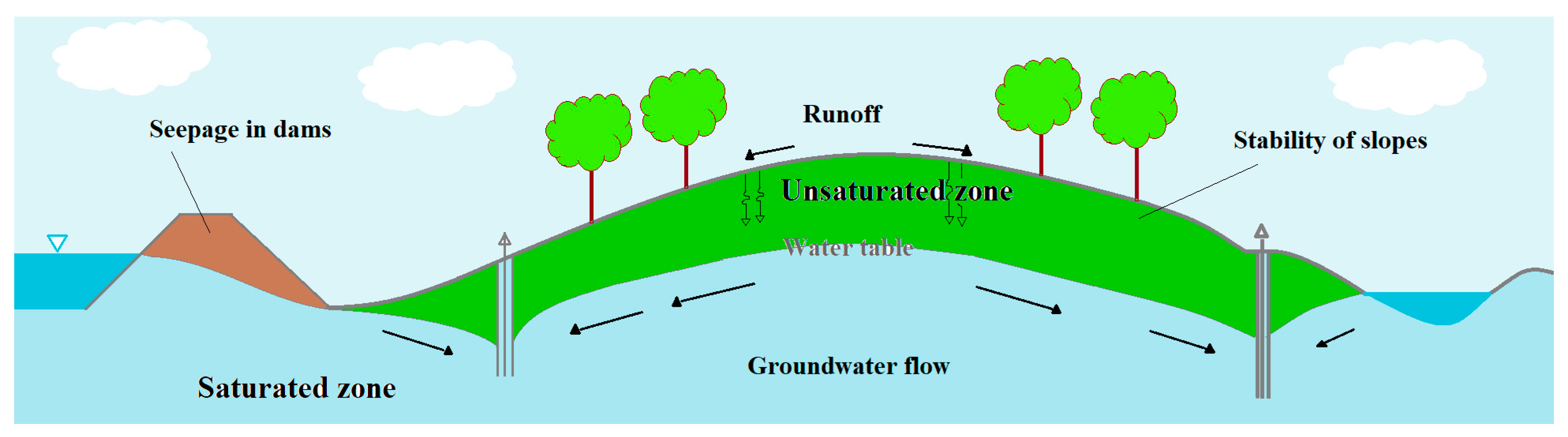
Figure 2.
Schematic of systematic selection of the database of current review based on PRISMA.

Figure 3.
Taxonomy of the review, soft computing methods in seepage modeling.

Figure 4.
Number of published papers employing soft computing methods in seepage simulation, extracted from Scopus.
Figure 4.
Number of published papers employing soft computing methods in seepage simulation, extracted from Scopus.

Figure 5.
Steps of seepage modeling via soft computing methods.

Figure 6.
Internal structure of LSTM unit, with five hidden units and an input dimension of 2 [86].
Figure 6.
Internal structure of LSTM unit, with five hidden units and an input dimension of 2 [86].
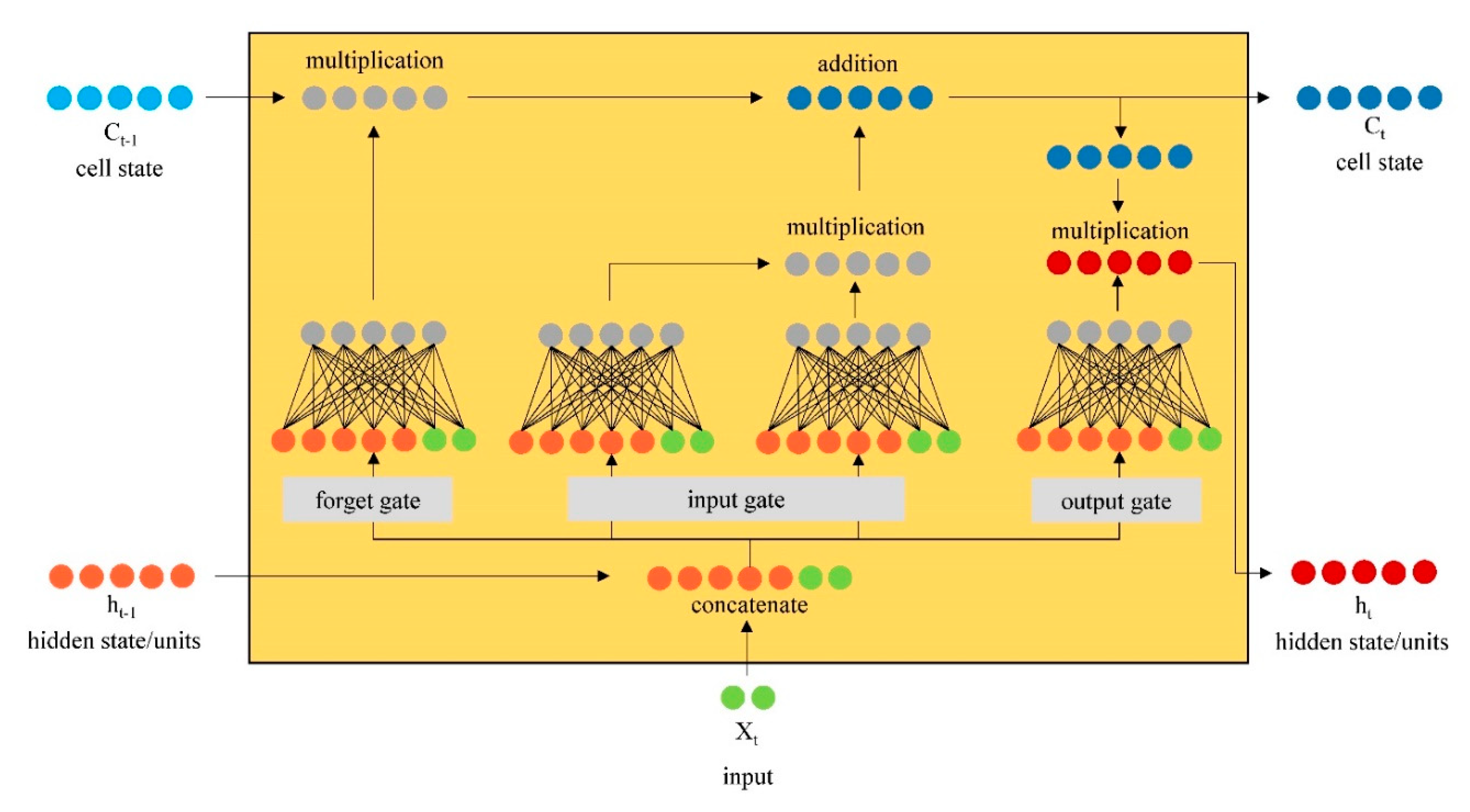
Figure 7.
The illustration of a sample CNN with two convolutions and one fully connected layer [88].
Figure 7.
The illustration of a sample CNN with two convolutions and one fully connected layer [88].

Figure 8.
Schematic of common hybrid soft computing methods for seepage modeling. (a) Wavelet-soft computing methods; (b) cluster-based soft computing methods; (c) evolutionary-soft computing methods; (d) soft computing geostatistic-based methods.
Figure 8.
Schematic of common hybrid soft computing methods for seepage modeling. (a) Wavelet-soft computing methods; (b) cluster-based soft computing methods; (c) evolutionary-soft computing methods; (d) soft computing geostatistic-based methods.
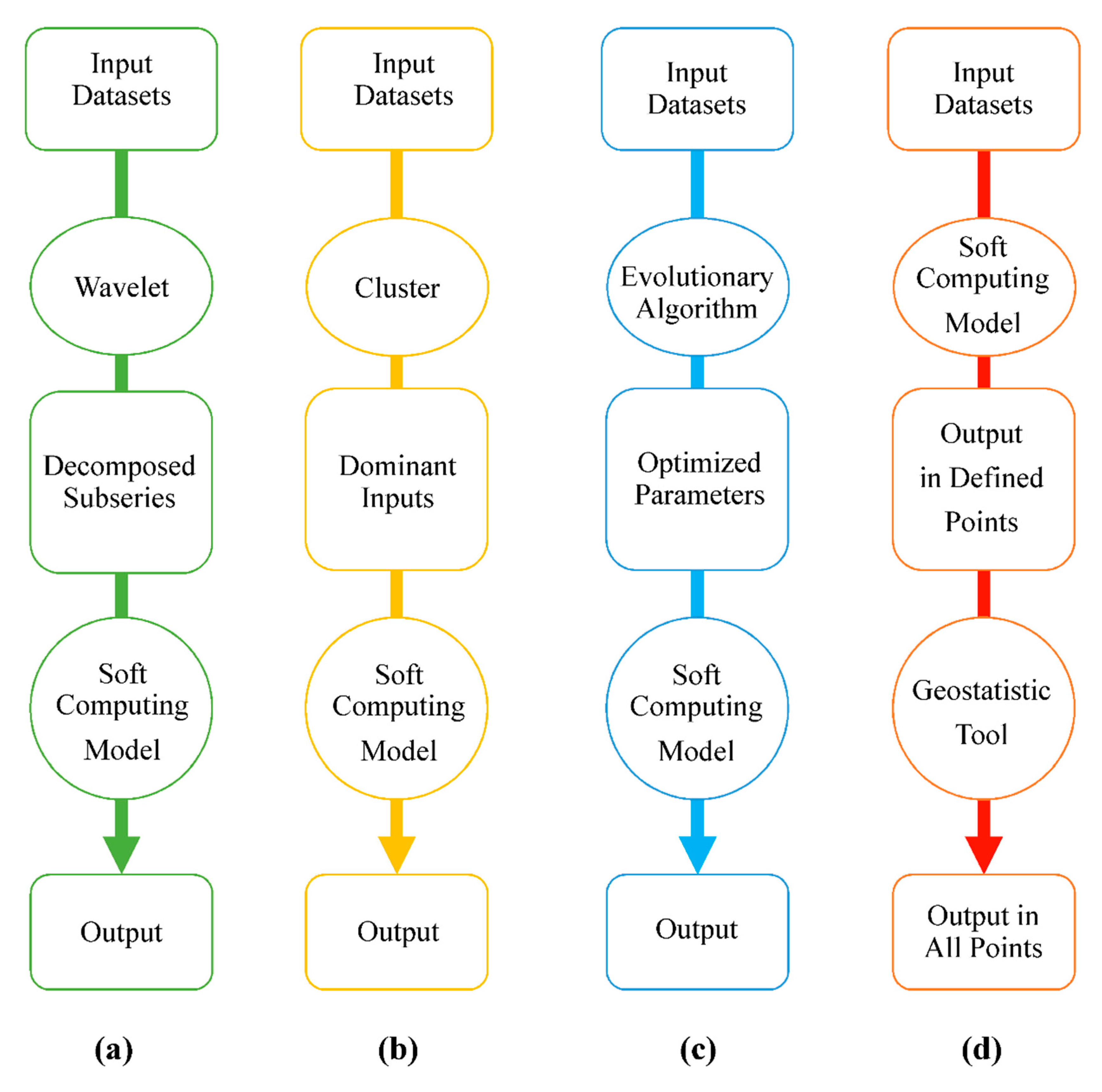
Figure 9.
Comparative performance analysis of single soft computing methods.

Figure 10.
Comparative performance analysis of hybrid soft computing methods.


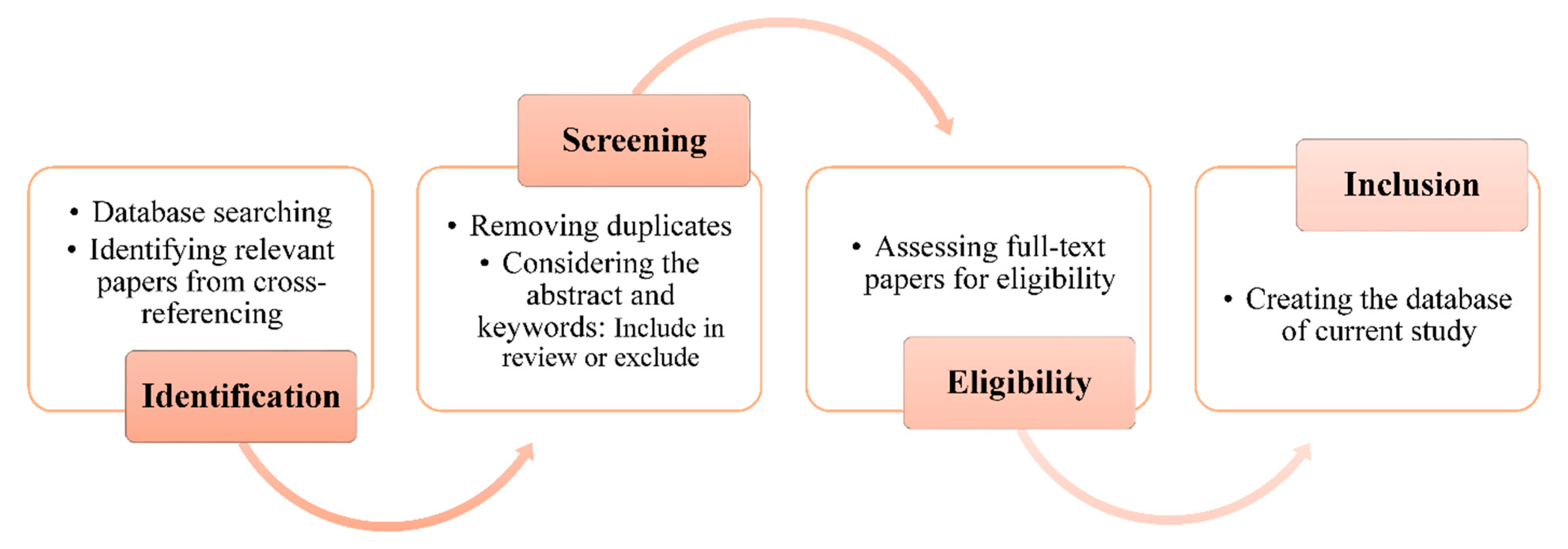
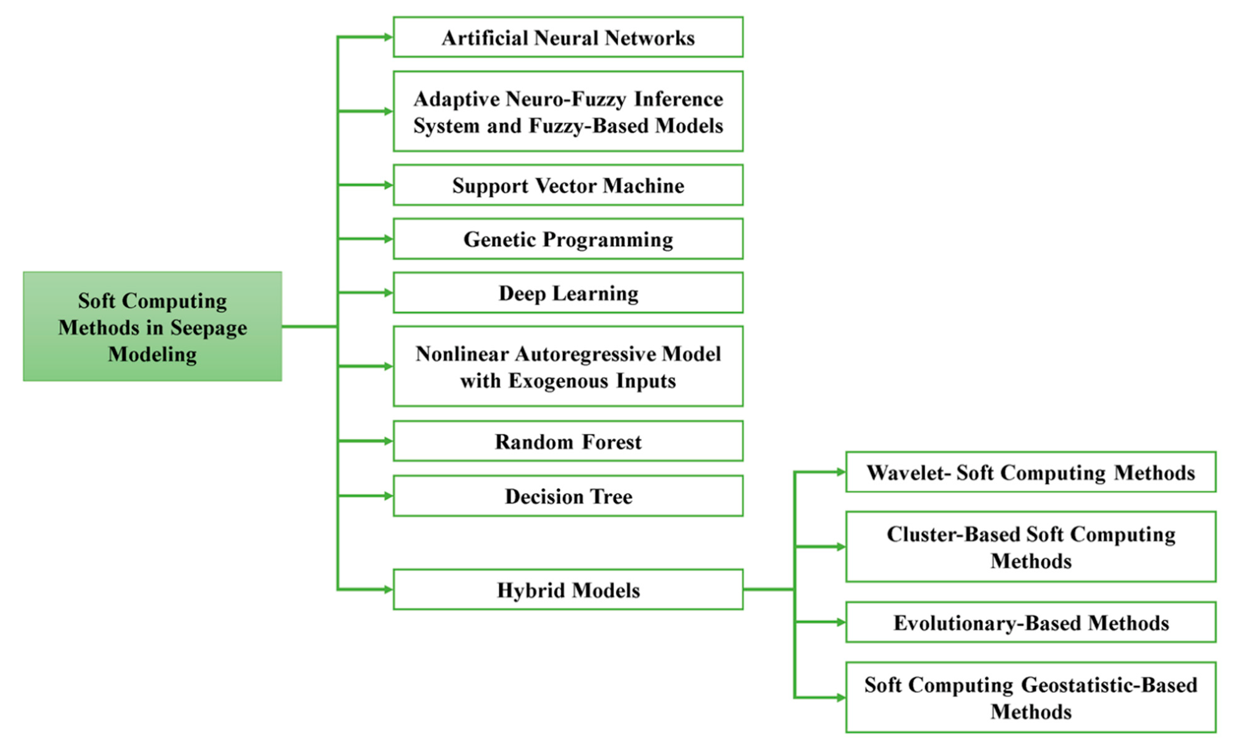
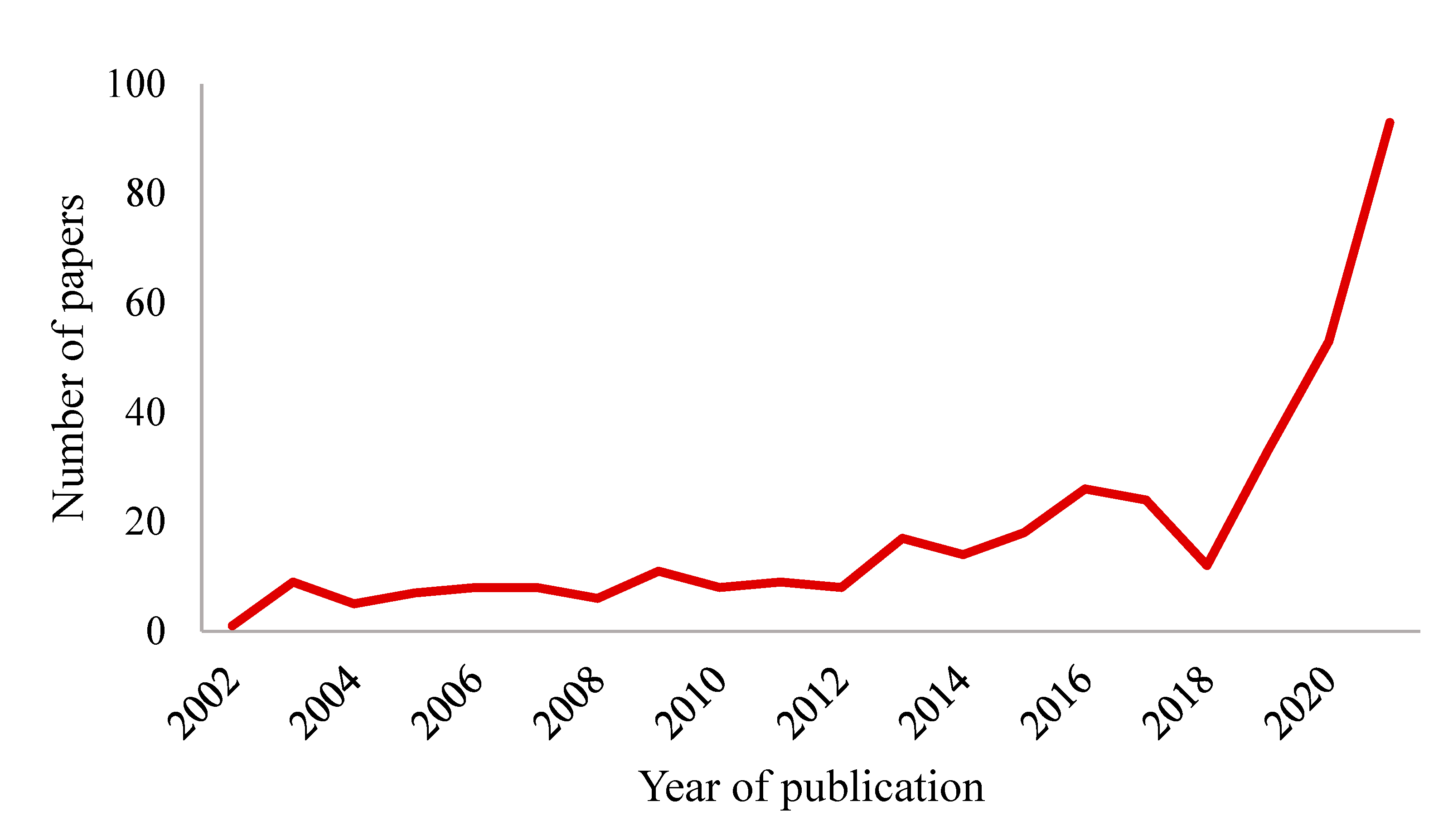
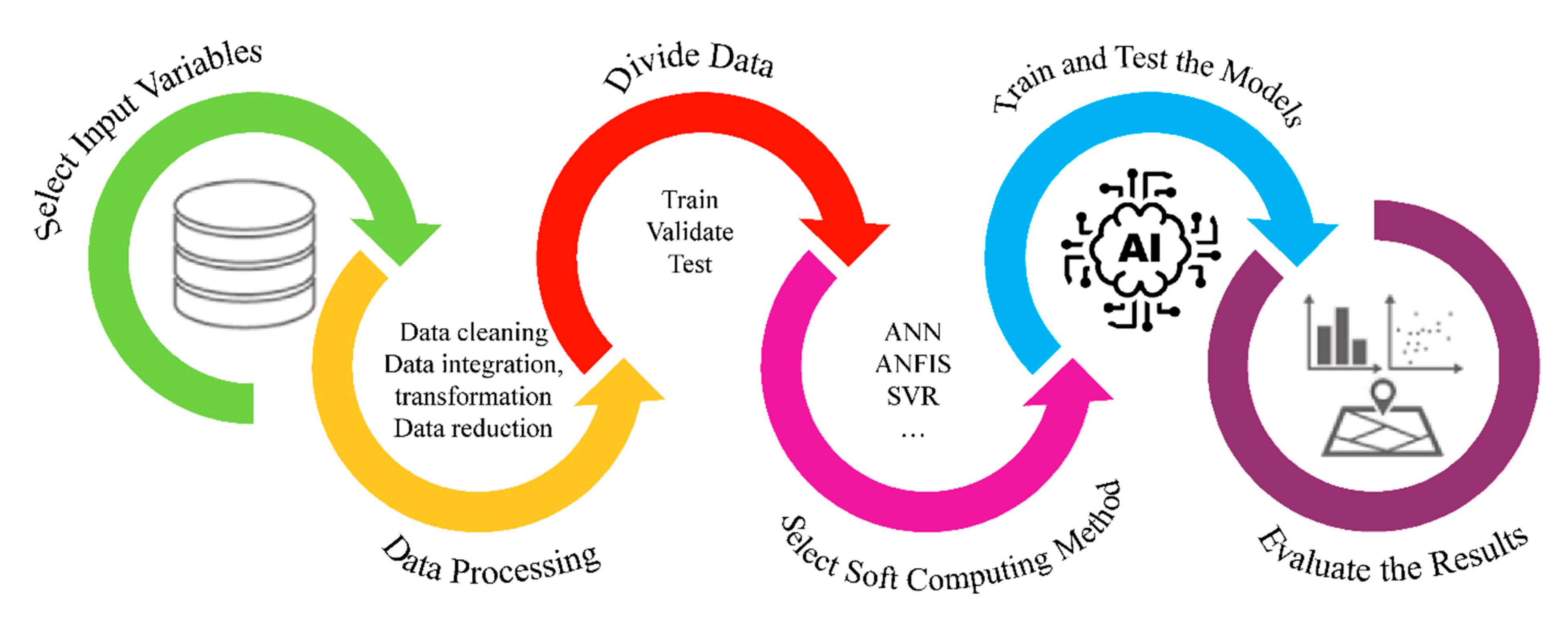
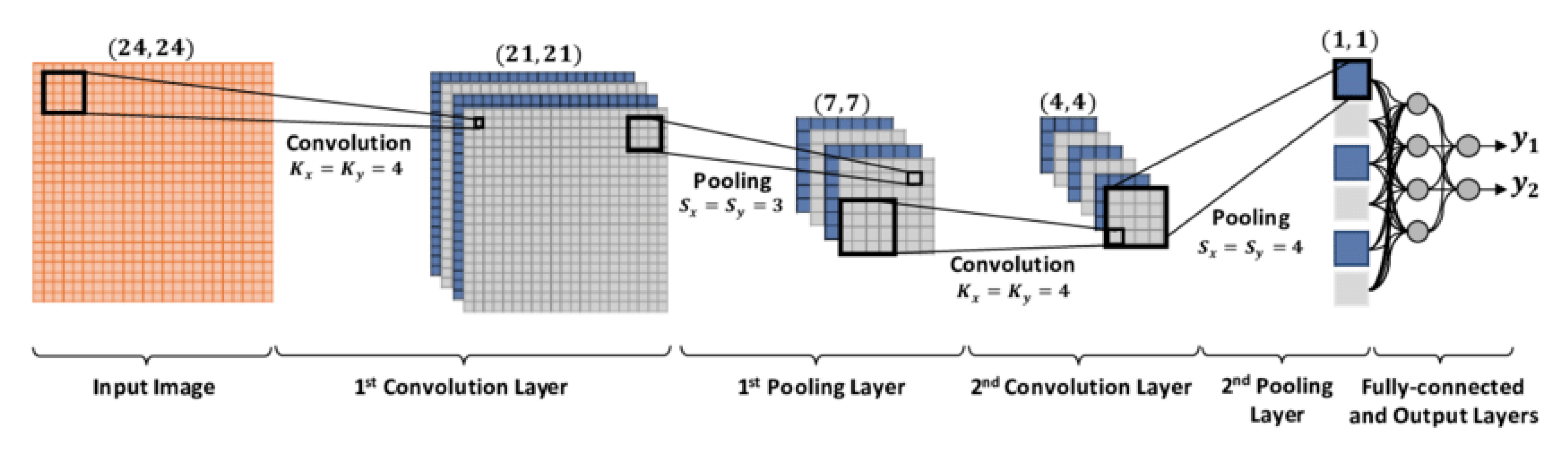
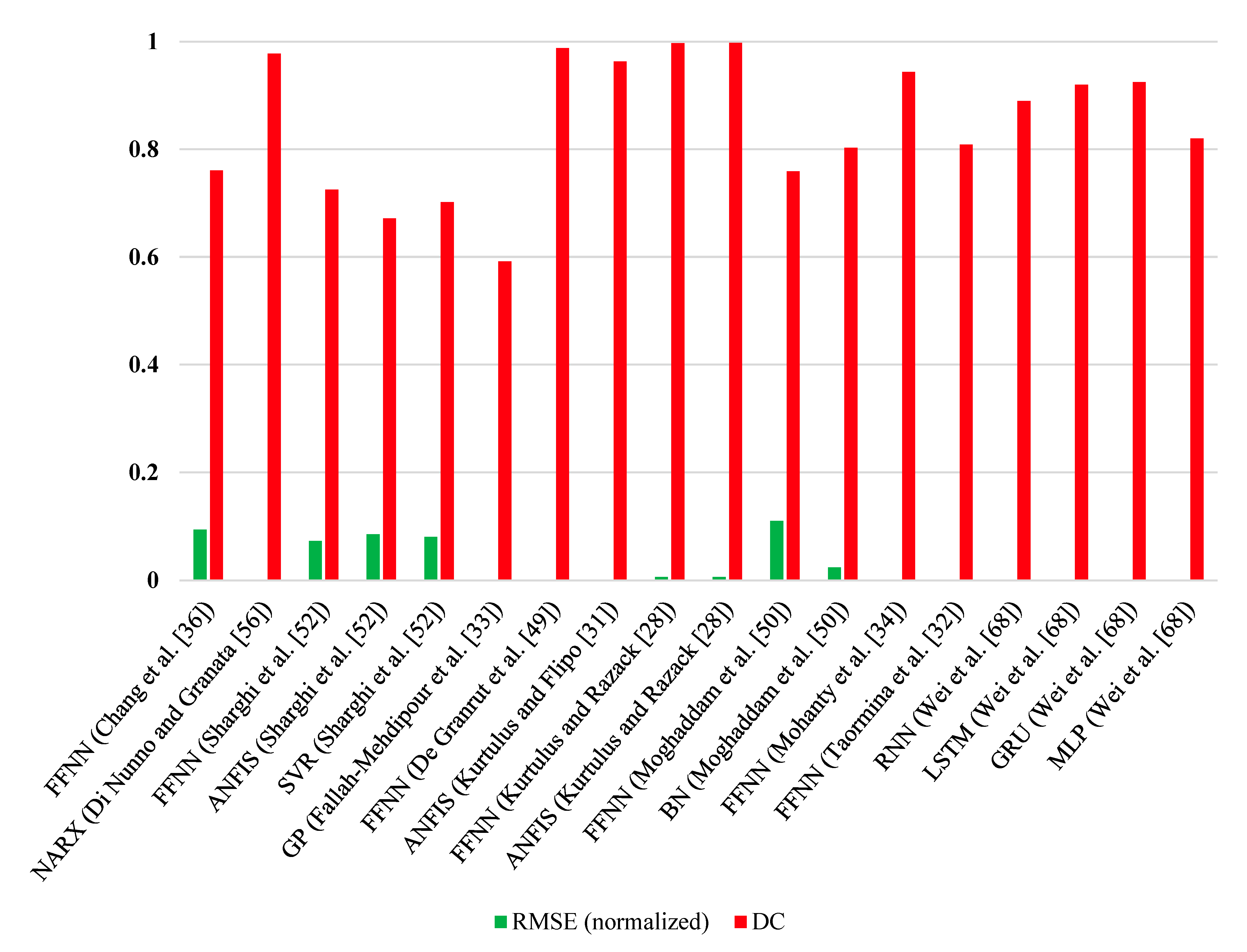
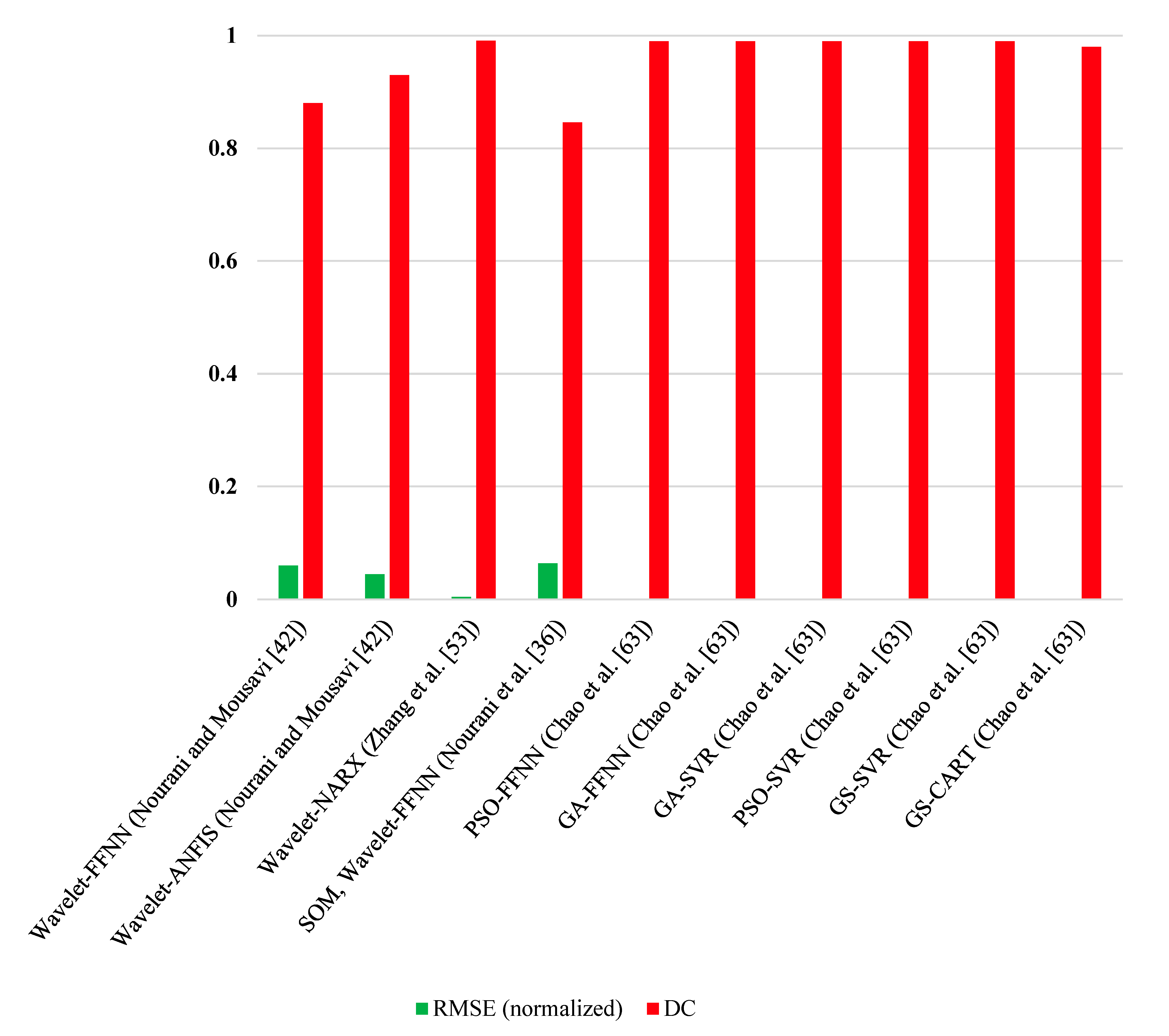
Table 1.
Details of the reviewed papers about application of soft computing methods in seepage modeling.
Table 1.
Details of the reviewed papers about application of soft computing methods in seepage modeling.
| No. | Authors Name | Publication Year | Employed Methods | Objectives | Journal Name | No. Citations |
|---|---|---|---|---|---|---|
| 1 | Balkhair [21] | 2002 | Feed forward neural network (FFNN) | Transmissivity and storage coefficient estimation | Journal of Hydrology | 57 |
| 2 | Lallahem et al. [22] | 2005 | Multilayer perception (MLP) | Groundwater levels estimation | Journal of Hydrology | 95 |
| 3 | Lin and Chen [23] | 2006 | FFNN | Transmissivity and storage coefficient estimation | Journal of Hydrology | 33 |
| 4 | Parkin et al. [24] | 2007 | FFNN | River–aquifer system modeling | Journal of Hydrology | 45 |
| 5 | Samani et al. [25] | 2007 | FFNN | Transmissivity and storage coefficient estimation | Journal of Hydrology | 82 |
| 6 | Hwang et al. [26] | 2009 | decision tree | Extract the rules of slope failure | Engineering Geology | 21 |
| 7 | Bashi-Azghadi et al. [27] | 2010 | Non-dominated sorting genetic algorithm-II (NSGA-II), Probabilistic support vector machine (PSVM), Probabilistic neural network (PNN) | Seepage detection from an unknown pollution source | Expert Systems with Applications | 49 |
| 8 | Kurtulus and Razack [28] | 2010 | FFNN, Adaptive neuro-fuzzy inference system (ANFIS) | Flow path estimation | Journal of Hydrology | 60 |
| 9 | Sun et al. [29] | 2011 | Backpropagation neural network (BPNN) | 3D hydraulic conductivity estimation | Tunnelling and Underground Space Technology | 31 |
| 10 | He et al. [30] | 2012 | FFNN | Dam foundation seepage simulation | Journal of Hydrodynamics, Ser. B | 5 |
| 11 | Kurtulus and Flipo [31] | 2012 | ANFIS | Hydraulic head estimation | Computers & Geosciences | 21 |
| 12 | Taormina et al. [32] | 2012 | FFNN | Groundwater levels estimation | Engineering Applications of Artificial Intelligence | 277 |
| 13 | Fallah-Mehdipour et al. [33] | 2013 | ANFIS, genetic programming (GP) | Obtaining the governing groundwater flow equations | Journal of Hydro-Environment Research | 95 |
| 14 | Mohanty et al. [34] | 2013 | FFNN | Groundwater flow estimation | Journal of Hydrology | 61 |
| 15 | Tapoglou et al. [35] | 2014 | FFNN, Fuzzy logic (FL), Kriging | Groundwater levels estimation | Journal of Hydrology | 48 |
| 16 | Chang et al. [36] | 2015 | FFNN | Groundwater levels estimation | Journal of Hydrology | 47 |
| 17 | Kaunda [37] | 2015 | FFNN | Internal erosion estimation | Computers and Geotechnics | 6 |
| 18 | Liu and Li [38] | 2015 | Genetic algorithm (GA) | Stability analysis and water-seepage modeling | Procedia IUTAM | 19 |
| 19 | Nourani et al. [39] | 2015 | Self-organizing map (SOM), Wavelet-FFNN, FFNN | Multi-scale patterns discovering of groundwater level | Journal of Hydrology | 72 |
| 20 | Zhou et al. [40] | 2015 | FFNN-GA | Transient groundwater flow estimation in dam foundation | Engineering Geology | 39 |
| 21 | Chang et al. [41] | 2016 | SOM, Nonlinear autoregressive model with exogenous inputs (NARX), Kriging | Groundwater levels estimation | Journal of Hydrology | 56 |
| 22 | Nourani and Mousavi [42] | 2016 | Wavelet-FFNN, Wavelet-ANFIS | Groundwater flow estimation | Journal of Hydrology | 36 |
| 23 | Shahrokhabadi et al. [43] | 2016 | Particle swarm optimization (PSO) | Solve the unconfined seepage problem | Computers & Mathematics with Applications | 3 |
| 24 | Hong et al. [44] | 2017 | FFNN, GA | Anisotropic hydraulic conductivity estimation | Computers and Geotechnics | 14 |
| 25 | Xiang et al. [45] | 2017 | PSO | Earth rock dam seepage modeling | Water Science and Engineering | 10 |
| 26 | Ghose et al. [46] | 2018 | Recurrent neural network (RNN) | Groundwater levels estimation | Groundwater for Sustainable Development | 15 |
| 27 | Wang et al. [47] | 2018 | Support vector regression (SVR) | Concrete gravity dam seepage modeling | Water Science and Engineering | 10 |
| 28 | Belmokre et al. [48] | 2019 | SVR | Dam seepage modeling | Procedia Structural Integrity | 1 |
| 29 | De Granrut et al. [49] | 2019 | FFNN | Uplift force analysis of an arch dam | Engineering Structures | 13 |
| 30 | Moghaddam et al. [50] | 2019 | FFNN, Bayesian network (BN) | Groundwater levels estimation | Groundwater for Sustainable Development | 17 |
| 31 | Rohmat et al. [51] | 2019 | Deep neural network (DNN), FFNN | Stream–aquifer exchange and water rights modeling | Environmental Modelling & Software | 3 |
| 32 | Sharghi et al. [52] | 2019 | FFNN, ANFIS, SVR | Earthfill dam seepage modeling | Measurement | 6 |
| 33 | Zhang et al. [53] | 2019 | Nonlinear input–output network (NIO), NARX, Wavelet-NARX | Groundwater levels estimation | Journal of Hydrology | 12 |
| 34 | Bao et al. [54] | 2020 | Generative adversarial network (GAN), Ensemble smoother with multiple data assimilation (ES-MDA) | Hydraulic head estimation | Journal of Hydrology | 1 |
| 35 | Chen et al. [55] | 2020 | Physics-guided neural network (PGNN), Convolutional neural network (CNN) | Water leak detection in canal sections | Advanced Engineering Informatics | 4 |
| 36 | Di Nunno and Granata [56] | 2020 | NARX | Groundwater levels estimation | Environmental Research | 13 |
| 37 | Liu et al. [57] | 2020 | SVR | Groundwater anomaly identification | Journal of Computational and Applied Mathematics | 4 |
| 38 | Panahi et al. [58] | 2020 | SVR, CNN | Developing the groundwater potential maps | Journal of Hydrology | 26 |
| 39 | Sun et al. [59] | 2020 | PSO-SVR | Determining the hydraulic aperture of rough rock fractures | Engineering Geology | 4 |
| 40 | Tao and Zheng [60] | 2020 | adaptive fuzzy identification | Seepage damage identification | Automation in Construction | 0 |
| 41 | Yu et al. [61] | 2020 | CNN | Pore characteristics analysis | Fuel | 8 |
| 42 | Chen et al. [62] | 2021 | Gated recurrent unit (GRU)-PSO | Groundwater flow estimation | Journal of Hydrology | 1 |
| 43 | Chao et al. [63] | 2021 | FFNN, SVR, Classification and regression tree (CART), Extreme learning machine (ELM), Grid search (GS)-CART, PSO-SVR, GA-SVR, GS-SVR, GA-FFNN, PSO-FFNN | Sandstone permeability estimation | Underground Space | 0 |
| 44 | Chen et al. [64] | 2021 | FFNN, GA | Permeability modeling of the foundation of a high arch dam | Journal of Rock Mechanics and Geotechnical Engineering | 0 |
| 45 | Daolun et al. [65] | 2021 | Signpost neural network (SNN) | Solving the seepage physics-constrained PDE | Journal of Petroleum Science and Engineering | 0 |
| 46 | Rehamnia et al. [66] | 2021 | FFNN | Embankment dam seepage modeling | Measurement | 4 |
| 47 | Zhang et al. [67] | 2021 | FFNN | Seepage modeling through the base of a dam | Alexandria Engineering Journal | 0 |
| 48 | Wei et al. [68] | 2021 | RNN, Long short-term memory (LSTM), GRU, MLP | Pore–water pressure estimation | Geoscience Frontiers | 10 |
Publisher’s Note: MDPI stays neutral with regard to jurisdictional claims in published maps and institutional affiliations. |
© 2021 by the authors. Licensee MDPI, Basel, Switzerland. This article is an open access article distributed under the terms and conditions of the Creative Commons Attribution (CC BY) license (https://creativecommons.org/licenses/by/4.0/).
Share and Cite
MDPI and ACS Style
Nourani, V.; Behfar, N.; Dabrowska, D.; Zhang, Y. The Applications of Soft Computing Methods for Seepage Modeling: A Review. Water 2021, 13, 3384. https://doi.org/10.3390/w13233384
AMA Style
Nourani V, Behfar N, Dabrowska D, Zhang Y. The Applications of Soft Computing Methods for Seepage Modeling: A Review. Water. 2021; 13(23):3384. https://doi.org/10.3390/w13233384
Chicago/Turabian StyleNourani, Vahid, Nazanin Behfar, Dominika Dabrowska, and Yongqiang Zhang. 2021. "The Applications of Soft Computing Methods for Seepage Modeling: A Review" Water 13, no. 23: 3384. https://doi.org/10.3390/w13233384
Note that from the first issue of 2016, this journal uses article numbers instead of page numbers. See further details here.