Atlantic Ocean Variability and European Alps Winter Precipitation

Abstract

Winter precipitation (snowpack) in the European Alps provides a critical source of freshwater to major river basins such as the Danube, Rhine, and Po. Previous research identified Atlantic Ocean variability and hydrologic responses in the European Alps. The research presented here evaluates Atlantic Sea Surface Temperatures (SSTs) and European Alps winter precipitation variability using Singular Value Decomposition. Regions in the north and mid-Atlantic from the SSTs were identified as being tele-connected with winter precipitation in the European Alps. Indices were generated for these Atlantic SST regions to use in prediction of precipitation. Regression and non-parametric models were developed using the indices as predictors and winter precipitation as the predictand for twenty-one alpine precipitation stations in Austria, Germany, and Italy. The proposed framework identified three regions in the European Alps in which model skill ranged from excellent (West Region–Po River Basin), to good (East Region) to poor (Central Region). A novel approach for forecasting future winter precipitation utilizing future projections of Atlantic SSTs predicts increased winter precipitation until ~2040, followed by decreased winter precipitation until ~2070, and then followed by increasing winter precipitation until ~2100.

1. Introduction

The Alps are often referred to as the “water towers” of Europe and provide a vital supply of freshwater to many of Europe’s most important rivers (e.g., Rhine, Po, Rhone) and tributaries of the Danube [1]. Snowpack accumulates during the winter months and melts during the warmer spring-summer season providing this critical resource. Thus, an understanding of winter precipitation variability in the European Alps is important for municipal water supply, energy (hydropower), agriculture and recreation (skiing).

Schöner et al. [2] examined Swiss-Austrian snow depth from 1961 to 2012 and seven spatiotemporal regions of snow depth were determined. Marty et al. [3] examined European Alps’ Snow Water Equivalent (SWE) and observed that the multi-decadal SWE decrease was independent of latitude or longitude despite the different climate regions in the Alpine domain. Increasing temperatures combined with a reduction in precipitation were the main drivers for the pronounced SWE loss [3] and snow loss (e.g., deteriorating snow conditions on ski slopes) could have a devastating impact on ski tourism [4]. Henderson and Leathers [5] and Kim et al. [6] evaluated European snow cover using satellite imagery over a ~40-year period. The North Atlantic Oscillation (NAO) was found to influence European snow cover with the negative NAO phase associated with snow cover increases whereas a positive NAO phase associated with snow cover decreases. The NAO signal was previously confirmed in winter (December to March) precipitation (1971 to 1992) over the Alpine region [7]. Scherrer and Appenzeller [8] examined winter (December-January-February or DJF) snowpack variability in Switzerland from 1958 to 1999 and identified the NAO in high-low elevation stations. Beniston [9] evaluated DJF precipitation in the Swiss Alps from 1931 to 2010 and identified declines which were also observed by Schöner et al. [10] in snowpack in the Sonnblick region (central Austrian Alps). Marcolini et al. [11] evaluated snow depth in the Adige catchment from 1980 to 2009 and identified a significant reduction in mean seasonal snow depth after 1988. Huss et al. [12] examined Swiss Alps glacial mass change in the 20th century. While considerable mass loss occurred during this period, the rates of mass loss varied with rapid periods of mass loss occurring in the 1940s and 1980s to present. The variability of mass loss was anticorrelated with the Atlantic Multidecadal Oscillation (AMO). Zampieri et al. [1] examined spring season snowfall in Switzerland, France and Italy using the Historical Instrumental Climatological Surface Time Series of the Greater Alpine Region (HISTALP) dataset. The spring snowfall transitioned from abundant to diminished during the mid-1990s, which coincided with the AMO transition from cold to warm phase and thus confirmed the AMO signal identified by Huss et al. [12].

Previous research efforts evaluated winter hydrology in the European Alps and generally supported the association of low-frequency variability of winter hydrology with the NAO and AMO. Several of these studies also support a recent multi-decadal decline in winter moisture in this region. The contributions of the current research will expand on these previous research efforts in at least three ways including:

• Precipitation stations were identified in Austria, Italy, and Germany and, per Scherrer and Appenzeller [8] and Beniston [9], the cumulative precipitation for the DJF season was selected. Per Zampieri et al. [1], the HISTALP database was selected for data mining and collection. Stations were selected from the HISTALP database with complete DJF data from 1950 to 2009 and elevations greater than 700 m. The authors attempted to identify multiple stations (longitudinally) in the European Alps to verify or discount AO climatic tele-connections.
• Previous studies evaluated AO climatic variability focusing on established AO climate signals (e.g., NAO and AMO). The use of AO SSTs eliminates any biases that are inherent in these pre-defined indices. Various statistical techniques exist to determine the relationship between two spatial-temporal fields including Singular Value Decomposition (SVD). In previous research efforts, Aziz et al. [13] applied SVD to identify Pacific Ocean SST influences on upper Colorado River snowpack in the western United States. As such, the SVD methodology was selected to evaluate European Alps’ DJF cumulative precipitation and AO SSTs.
• Regression (Stepwise (Forward and Backward) Linear Regression or SLR) and non-parametric (NP) models were developed such that the predictand (dependent variable) was DJF precipitation while the predictors (independent variables) were indexes (e.g., the North Atlantic Index or NAI for the north AO SST region and the Mid Atlantic Index or MAI for the mid AO SST region) developed per the SVD analysis. In prior research efforts, NP forecast models were developed utilizing Pacific Ocean climatic variability (as derived by SVD) to forecast seasonal snowpack (April 1st SWE) in the western United States [14] and this approach was applied in the current research efforts. In lieu of developing annual forecast models, the motivation of the current research was to capture the low-frequency variability of AO climate and European Alps winter precipitation. As such, both predictand (DJF precipitation) and predictors (MAI and NAI) were smoothed (20-year end-year filter). Thus, if skillful SLR and NP model forecasts are developed, the ability to capture this low frequency variability (with uncertainty) would allow the incorporation of future climate predictions of the AO SSTs into these “trained” SLR and NP models, which can avoid uncertainties in multi-decadal variability of simulated precipitation of climate models [15]. This could lead to a novel approach in that, based on various climate change scenarios, future AO SST variability is utilized, and future multi-decadal forecasts of winter precipitation are determined and could be compared to forecasts using traditional approaches.

The overall objective of the study presented here is to evaluate the potential of using Atlantic Ocean sea surface temperatures (SSTs) to enhance the projections of precipitation for the European Alps under changing climate conditions. Following is a detailed description of the materials (data) and methods, presentation of the results and discussion/conclusions.

2. Materials and Methods

2.1. Study Data

The HISTALP database was accessed and 21 stations were identified in Austria, Italy, and Germany [16] (Figure 1a,

Table 1. ID, Station Name, Country, Latitude, Longitude, Elevation (meters), Coefficient of Determination (R2), average Cross-Validated (CV) Linear Error in Probability Space (LEPS) score and Region for 21 stations selected in current research. Stations with R² > 40% and CV LEPS > 10 are shaded.

ID	Station Name	Country	Latitude	Longitude	Elevation	R2	CV LEPS	Region
1	Badgastein	Austria	47.1	13.1	1092	29.3%	2.4	East
2	Bad Bleiberg	Austria	46.6	13.7	907	61.9%	24.2	East
3	Döllach	Austria	47.0	12.9	1078	62.8%	−2.1	East
4	Kals	Austria	47.0	12.6	1338	48.4%	7.1	East
5	Langen	Austria	47.1	10.1	1221	NA	2.6	Central
6	Nauders	Austria	46.9	10.5	1360	NA	7.8	Central
7	Rauris	Austria	47.2	13.0	941	16.4%	−2.5	East
8	Tamsweg	Austria	47.1	13.8	1025	55.6%	11.8	East
9	Obervellach-Flattach-Kleindorf	Austria	46.9	13.2	809	57.4%	27.6	East
10	Radstadt	Austria	47.4	13.5	858	62.5%	6.4	East
11	Seckau	Austria	47.3	14.8	855	NA	5.9	NA
12	St. Sebastian	Austria	47.8	15.3	872	47.8%	4.7	NA
13	Millstatt	Austria	46.8	13.6	719	68.0%	18.8	East
14	Zell am See	Austria	47.3	12.8	766	41.7%	11.9	East
15	Balme	Italy	45.3	7.2	1432	69.0%	32.2	West
16	Ceresole Reale	Italy	45.4	7.3	1579	63.9%	23.1	West
17	Formazza Ponte	Italy	46.4	8.4	1300	58.0%	29.4	NA
18	Lemie-C.le.	Italy	45.2	7.3	940	64.0%	24.7	West
19	Marienberg/Montemaria	Italy	46.7	10.5	1323	18.9%	−7.0	Central
20	Hohenpeißenberg	Germany	47.8	11.0	986	10.2%	−0.3	Central
21	Oberstdorf	Germany	47.4	10.3	810	47.8%	−2.2	Central

). The period of 1950 to 2009 (60 years) was selected for the analysis based on availability of monthly data, and stations are at a minimum elevation of 700 m. While the primary criteria for data selection was data availability, period of record, and elevation, the authors attempted to identify a large, spatial region from east (i.e., Italy) to west (i.e., Austria) to account for any variations in climatic variability (Figure 1a, Table 1). Given the physical location of the European Alps, the variation in latitude of these stations was only ~2.5-degrees while the variation in longitude was ~8.0-degrees. While the varying geography could contribute to “noise” in attempting to establish an interdecadal climate signal, the selected stations represent a robust, spatially un-biased dataset for the analysis. Cumulative DJF precipitation (millimeters) was obtained such that the 1950 data represents December 1950 and January–February 1951 while the 2009 data represents December 2009 and January–February 2010.

The NOAA Extended Reconstructed SST version 3b was downloaded from the NOAA Earth System Research Laboratory (ERSST v3b) [17]. The monthly ERSST SST averages are at the 200-km spatial resolution and cover 1854–2019. In this study, the regional SST averages spanning from 20° South to 70° North and 80° West to 2° West were computed. The defined region includes 1239 grid cells over the AO. The averages of AO SSTs were calculated for six predictor seasons (JFMAMJ—5-month lead-time, FMAMJA—4-month lead-time, MAMJJA—3-month lead-time, AMJJAS—2-month lead-time, MJJASO—1-month lead-time and JJASON—0-month lead-time). In this study, the AO SST data period of record was 1950 to 2009 (60 years). The selection of the six-month seasons (e.g., JFMAMJ, FMAMJJ, MAMJJA, AMJJAS, MJJASO, and JJASON) for AO SSTs was justified based on previous research presented in [13] and [14] in which six-month seasons (e.g., JFMAMJ, AMJJAS, and JASOND) were selected. The period of record (e.g., 1950 to 2009—60 years) was selected based on availability of complete data for all stations selected. The 60 year period is similar in record length to [13] (1961 to 2006—46 years) and [14] (1961 to 2002—42 years).

Future AO SSTs were obtained from the Shared Socioeconomic Pathway (SSP) (1.26 (best) or 5.85 (worst) scenario runs) of the Coupled Inter-comparison Model Project Phase 6 (CMIP6) [18]. These future projections of AO SSTs were used to generate the future Mid-Atlantic and North Atlantic Indexes (MAI and NAI, respectively). Five CMIP6 models were selected due to the data availability and were included: CCCma-CanESM5 (20, 20), CNRM-CM6-1 (6, 6), CNRM-ESM2-1 (5, 5), IPSL-CM6A-LR (3, 1), MIROC6 (3, 3), MRI-ESM2-0 (1, 1), and NASA-GISS-E2-1-G (5, 5) and the ensemble sizes of the SSP1.26 (43 total) and SSP5.85 (41 total) of the CMIP6 models are provided within parenthesis after each model identifier.

2.2. Methods—Singular Value Decompostion (SVD)

SVD is a powerful statistical tool for identifying coupled relationships between two, spatial-temporal fields, as Sadeghi et al. [19] identified 18 prior climate studies in which SVD was applied. Bretherton et al. [20] and Wallace et al. [21] provide a detailed discussion of the theory of SVD and a brief description of SVD, as applied in the current research, is hereby provided. Initially, a matrix of standardized AO SST anomalies and a matrix of standardized DJF precipitation anomalies were developed. The time dimension of each matrix (i.e., 60 years) must be equal while the spatial component (i.e., AO SST cells and precipitation stations) can vary in dimension. The cross-covariance matrix was then computed for the two spatial, temporal matrices and SVD was applied to the cross-covariance matrix and physical information regarding the relationship between the two was obtained. The resulting SVD of the cross-covariance matrix created two matrices of singular vectors and one matrix of singular values. The singular values were ordered such that the first singular value (1st mode) was greater than the second singular value and so on. Bretherton et al. [20] defines the squared covariance fraction (SCF) as a useful measurement for comparing the relative importance of modes in the decomposition. Each singular value was squared and divided by the sum of all the squared singular values to produce a fraction (or percentage) of squared covariance for each mode. Finally, the two matrices of singular vectors were examined, generally referred to as the left (i.e., AO SSTs) matrix and the right (i.e., precipitation) matrix. The first column of the left matrix (1st mode) was projected onto the standardized AO SSTs anomalies matrix and the first column of the right matrix (1st mode) was projected onto the standardized precipitation anomalies matrix. This resulted in the 1st temporal expansion series of the left and right fields, respectively. The left heterogeneous correlation values (for the 1st mode) were determined by correlating the AO SST values of the left matrix with 1st temporal expansion series of the right field and the right heterogeneous correlation values (for the 1st mode) were determined by correlating the precipitation values of the right matrix with the 1st temporal expansion series of the left field. Utilizing a similar approach to [21], Rajagopalan et al. [22] and Uvo et al. [23], heterogeneous correlation figures were developed for each of the six predictor seasons and a “composite” figure was developed highlighting AO SST cells which achieved an average significance of 95% and 99% when averaging the six predictor seasons. Using the significant cells identified and the corresponding SST values, an index (e.g., NAI or MAI) was developed annually for 1950 to 2009. These indexes were detrended and smoothed (20-year end-year filter).

2.3. Methods—Stepwise Regression Model for Precipitation

The ability of the MAI and NAI to predict winter (DJF) precipitation was tested using a forward and backward (standard) stepwise regression model (SLR). SLR adds and removes predictors, as needed, for each step. The model stops when all variables not in the model have p-values that are greater than the specified alpha-to-enter value and when all variables in the model have p-values that are less than or equal to the specified alpha-to-remove value. Per Anderson et al. [24], the F-level for a predictor had to have a maximum p-value of 0.05 for entry and 0.10 for retention in our stepwise regression model. Numerous statistical measures were used to establish the statistical skill. R² provides the amount of variance explained by each model while predicted R² is based upon a leave-one-out cross-validation. The Variation Inflation Factor (VIF) indicates the extent to which multicollinearity is present and a value close to one (1.0) indicates low correlation between predictors and is ideal for a regression model.

2.4. Methods—Non-Parametric Model for Precipitation

The precipitation prediction developed by the non-parametric (NP) model is a continuous exceedance probability curve that can be used for any assumed risk level and a detailed description of the model can be found in Piechota et al. [25] and Piechota et al. [26]. Two advantages are that it considers the continuous relationship between the predictand and the predictor and it does not assume a specific model structure. The skill of the forecast, as produced by the model, was measured using the Linear Error in Probability Space (LEPS) score. The LEPS score is a measure of skill that was originally developed to assess the position of the forecast and the position of the observed values in the cumulative probability distribution (non-exceedance probability) and can be used for continuous and categorical variables [27,28]. A modified LEPS score is required due to the absence of a convenient measure of skill for an exceedance probability forecast. A better measure of skill is one in which more weight is given to a forecast that effectively predicts low or high flow and less weight to a forecast that successfully predicts average flow. The application of the LEPS score is desirable here because it is less sensitive to changes near the center of the cumulative probability distribution and more sensitive to forecasts of high or low values. Essentially, it rewards a successful forecast of extreme value [25]. The LEPS score for the calibration analysis does not provide an independent skill score because it is based on the same data in which the model was calibrated and thus a cross validated LEPS skill score (CV LEPS) was developed. To report the skill scores explained in the results section, each individual annual CV LEPS was averaged over the entire period of record to develop an overall average forecast skill. If the CV LEPS score average exceeds +10, the model is considered to have good skill [27,28] A negative CV LEPS score indicates a model that performs worse than simply selecting the 50th percentile for all forecasts.

2.5. Future Scenarios of AO, NAI and MAI

For future AO SSTs, the ensemble means (EMs) of 41 and 43 ensemble members of the SSP1.26 and SSP5.85 runs were computed by the averages of the ensemble mean of each model (the “one vote for one model” rule). The smoothing effect of 41 or 43 ensemble runs caused underestimation of the standard deviations of the detrended SSTs but the general response to climate change still remains. Therefore, the mean and variability adjustment (bias correction, BC) in the future SSTs were conducted, following the method of Kam et al. [29]. First, the raw MAI and NAI were detrended and then weighted by the ratio of the standard deviations of the observed SSTs (1951–2016) to the standard deviations of the detrended SSTs (2017–2100). The weights for MAI and NAI were three and five, respectively, which were not affected by the future scenarios. The linear trends were added in the bias-corrected SSTs. The slopes of the SSP1.26 (SSP5.85) runs were 0.8 and 1 °C (4 and 6.5 °C) per century for MAI and NAI, respectively. Lastly, the BC MAI and NAI of the SSP1.26 (SSP5.85) runs were subtracted by 1 and 0.3 °C (3 and 2.6 °C), respectively, to avoid the gap between the index values of 2016 (the last year of the observed indexes) and 2017 (the start year of the future indexes).

3. Results

3.1. SVD Analysis of Atlantic SSTs

SVD (1st mode based on SCF values) identified two regions in the AO that were tele-connected with winter precipitation (Figure 1b). Figure 1b was derived from the SVD analysis for the six predictor seasons (JFMAMJ—5-month lead-time, FMAMJA—4-month lead-time, MAMJJA—3-month lead-time, AMJJAS—2-month lead-time, MJJASO—1-month lead-time and JJASON—0-month lead-time) and represents a composite map of AO SST cell correlations (significance). The region in the north AO (light gray ~95% significance) appears to be AMO-like while the region in the mid AO (dark gray ~99% significance) represents a unique tele-connection with winter precipitation. Indexes were created for each region (e.g., the North Atlantic Index or NAI for the north AO SST region and the Mid Atlantic Index or MAI for the mid AO SST region) and, each index was detrended and smoothed (20-year filter). The AMO is defined as the leading mode of low-frequency, north AO (0 degree to 70 degree) SST variability with a periodicity of 65–80 years [30,31]. The AMO index consists of detrended SST anomalies and AMO index values were available from the National Oceanic and Atmospheric Administration (NOAA) [32]. Applying a 20-year end-year filter and comparing the AMO index to the NAI index, the Coefficient of Determination (R²) was 90%. Thus, SVD confirmed the AMO signal in European Alps winter precipitation.

3.2. SLR and NP Model Results

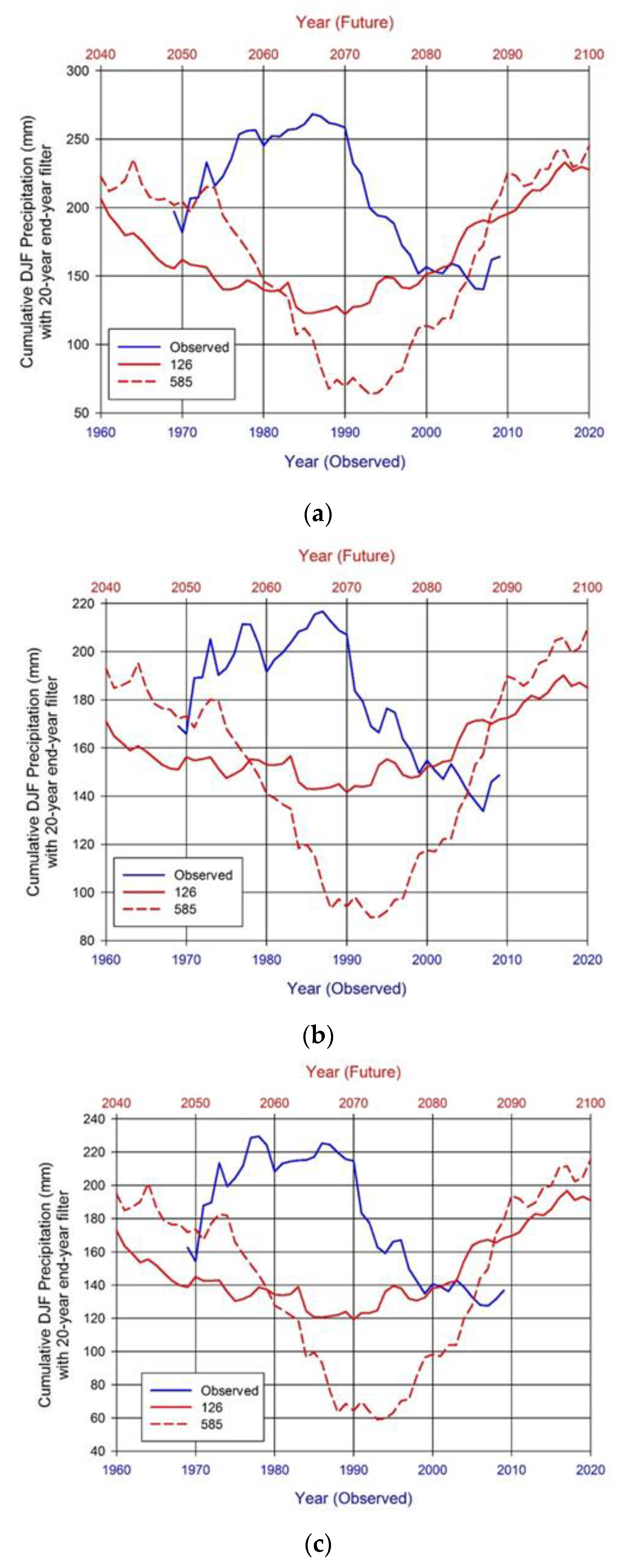
For each station, 1950 to 2009 DJF cumulative precipitation was smoothed (20-year end-year filter) and, thus, forecasts (using SLR and NP models) were determined for 1969 to 2009. For the SLR models, statistical skill was evaluated by examining R², R² predicted and VIF while statistical skill for NP models was evaluated by examining the average CV LEPS score. For each station, the SLR model R² value and the NP model average CV LEPS score value was provided in Table 1. For the SLR models, while subjective, the author’s deemed an R² threshold value exceeding 40% to be considered skillful. As previously stated, if the CV LEPS score average exceeds +10, the model is considered to have good skill [27,28].

Referring to Table 1 and Figure 1a, the results of the SLR and NP models generally reflect three spatial regions in which excellent, good, and poor forecast skill were determined. Five stations were identified as being spatially located in the central region (Table 1 and Figure 1a) and the average R² for these stations was 25.6% while the average CV LEPS score was +0.2. Thus, the forecast skill in the central region was poor. Ten stations were identified as being spatially located in the east region (Table 1 and Figure 1a) and the average R² for these stations was 50.4% while the average CV LEPS score was +10.6. Thus, the forecast skill in the east region was good. Three stations were identified as being spatially located in the west region (Table 1 and Figure 1a) and the average R² for these stations was 65.6% while the average CV LEPS score was +26.7. Thus, the forecast skill in the west region was excellent. Stations 11, 12 and 17 were considered (spatially) to be outliers. The three stations in the west region are all located in Italy and within the Po River basin. The Po River is Italy’s longest river (~650 km) and flows easterly before ending in the Adriatic Sea near Venice and has a drainage area of ~74,000 km². The Po River provides a vital water and energy (hydropower) source for northern Italy. Thus, given the importance of European Alps snowmelt to the Po River, an understanding of the variability of winter precipitation and the AO SST drivers of this variability may prove valuable in water planning and management.

Referring to Figure 2, a detailed review of the results of the west region (Po River basin) stations is hereby provided:

• Balme

  ○

  SLR Model: R² = 69.0%, R2 predicted = 65.4% and VIF = 1.2. The model underestimated DJF during the 1980 to 1990 period while overestimating DJF during the 1990 to 2000 period (Figure 2a). The regression model is DJF = 182.68 + 101.4 MAI − 143.6 NAI. Given both indexes are standardized, slightly more weight was placed on the northern AO SST region (i.e., AMO like SST region).

  ○

  NP Model: CVLEPS = +32.2. Other than an anomalous low value in 1984, the model performed well when compared to observed DJF (Figure 2a)

• Ceresole Reale

  ○

  SLR Model: R2 = 63.9%, R² predicted = 59.5% and VIF = 1.2. The model underestimated DJF during the 1980 to 1990 period while overestimating DJF during the 1990 to 2000 period (Figure 2b). The regression model is DJF = 165.79 + 68.4 MAI − 81.84 NAI, thus, the weights on each predictor were similar.

  ○

  NP Model: CVLEPS = +23.1. There was an anomalous low value (0) in 1970 (not displayed in Figure 2b) and an anomalous low value in 2009 (Figure 2b).

• Lemie-C.le.

  ○

  SLR Model: R2 = 69.0%, R² predicted = 59.8% and VIF = 1.2. The model underestimated DJF during the 1980 to 1990 period while overestimating DJF during the 1990 to 2000 period (Figure 2c. The regression model is DJF = 159.84 + 88.5 MAI − 114.2 NAI, thus, the weights on each predictor were similar.

  ○

  NP Model: CVLEPS = +24.7. There were anomalous low values in 1969, 1970 and 2009 (not displayed in Figure 2c).

The NP model did display some challenges with anomalous low values, particularly at the beginning and end of the period of record, but both the SLR and NP models displayed excellent skill and generally captured the temporal variability of DJF precipitation. The low skill of the NP model is likely to be a reflection of the sensitivity of this approach to the initial (or ending) conditions used as it is a non-parametric approach that uses nearest neighbors.

Applying the SLR models previously developed, future forecasts (2040 to 2100) of DJF were developed using the future NAI and MAI indexes (as developed for both SSP1.26 and 5.85 scenarios) and compared to the observed record (1969 to 2009) (Figure 3). The future forecasts predict a period of declining DJF precipitation from ~2040 to ~2070 followed by a period of rising DJF precipitation from ~2070 to ~2100. Each station identified the decline in the SSP 5.85 runs to be more severe than the SSP 1.26 runs. While the predicted decline from ~2040 to ~2070 is significant, it should be noted for the 5.85 scenario, the magnitude of 2040 (60 to 75 mm)is greater than the 2009 observation for each station while the SSP1.26 scenario show a similar magnitdue in 2040 (120 to 145 mm) to the observed in 2010s. This result indicates that the future risk of unprecedented dry decades, particularly for wintertime precipitation, over the Alps would depend on the selection of future scenarios. Thus, we suspect a period of rising DJF in the next ~20 to ~30 years which may coincide with the AMO shift from warm to cold phase. The different phases represented in the blue and red lines are likely to correspond to shifts that occur in AMO phases The observed (blue line) and future (red line) were overlayed in Figure 3 (note time-scales at both top and bottom of figures) to provide a comparison of these shifts and the difference in DJF magnitudes in observed and future precipitation.

4. Discussion

The current research identified recent declines in DJF precipitation, thus confirming the observations of Marty et al. [3], Beniston [9] and Schöner et al. [10] (Figure 2). The Po River basin (West Region) stations displayed exceptional skill in both SLR and NP models. Each station retained the newly developed MAI, thus the identification of the mid Atlantic Ocean SST region by SVD and the subsequent development of the MAI index to represent this region contributed and improved model skill. A further review of Figure 2 clearly reveals the influence of the AMO (i.e., NAI) on winter precipitation in this region. From the beginning of the record until ~1990, there is a steady rise (increase) in DJF precipitation and this corresponds with the AMO cold phase. In the early 1990s, as the AMO shifted to a warm phase, a steady decline (decrease) in DJF precipitation was observed. It is also noteworthy to compare these findings to those of the IPCC projections [33] which show the difference of the 20-year averages of DJF precipitation between the past (1995–2014) and future (2081–2100). The 20-year averages (red lines) from Figure 3 of the current study were similar to those findings in the IPCC report of increased DJF precipitation in northern Italy for 2081–2100 [33].

5. Conclusions

The current research provides a new and novel approach in the utilization of future AO SST variability to forecast future DJF precipitation variability. In addition, it is noteworthy that high skill was obtained for precipitation. The research is limited in that the variability in precipitation is only represented by the larger scale climate (i.e., Atlantic Oceanic influence). In addition, the research does not account for local influences that may act at shorter time scales. Regardless, the potential of prediction future precipitation has implication for identifying changes in water supply in these regions. Future research could focus on water supply (i.e., streamflow) forecasts which have been shown to be an integrator of the hydrologic processes and better tele-connected to climate variables. Regardless, these future predictions of DJF precipitation can be compared to those from traditional climate change forecasts and provide an additional tool for water managers and planners.

References

1. Zampieri, M.; Scoccimarro, E.; Gualdi, S. Atlantic influence on spring snowfall over the Alps in the past 150 years. Environ. Res. Lett. 2013, 8, 034026. [Google Scholar] [CrossRef]
2. Schöner, W.; Koch, R.; Matulla, C.; Marty, C.; Tilg, A.-M. Spatiotemporal patterns of snow depth within the Swiss-Austrian Alps for the past half century (1961 to 2012) and linkages to climate change. Int. J. Clim. 2018, 39, 1589–1603. [Google Scholar] [CrossRef]
3. Marty, C.; Tilg, A.-M.; Jonas, T. Recent Evidence of Large-Scale Receding Snow Water Equivalents in the European Alps. J. Hydrometeorol. 2017, 18, 1021–1031. [Google Scholar] [CrossRef]
4. Steiger, R.; Posch, E.; Tappeiner, G.; Walde, J. The impact of climate change on demand of ski tourism—A simulation study based on stated preferences. Ecol. Econ. 2020, 170, 106589. [Google Scholar] [CrossRef]
5. Henderson, G.R.; Leathers, D.J. European snow cover extent variability and associations with atmospheric forcings. Int. J. Clim. 2009, 30, 1440–1451. [Google Scholar] [CrossRef]
6. Kim, Y.; Kim, K.-Y.; Kim, B.-M. Physical mechanisms of European winter snow cover variability and its relationship to the NAO. Clim. Dyn. 2012, 40, 1657–1669. [Google Scholar] [CrossRef]
7. Quadrelli, R.; Lazzeri, M.; Cacciamani, C.; Tibaldi, S. Observed winter Alpine precipitation variability and links with large-scale circulation patterns. Clim. Res. 2001, 17, 275–284. [Google Scholar] [CrossRef]
8. Scherrer, S.C.; Appenzeller, C. Swiss Alpine Snow Pack Variability: Major Patterns and Links to Local Climate and Large-Scale Flow. Clim. Res. 2006, 32, 187–199. [Google Scholar] [CrossRef] [Green Version]
9. Beniston, M. Is Snow in the Alps Receding or Disappearing? Clim. Chang. 2012, 3, 349–358. [Google Scholar] [CrossRef] [Green Version]
10. Schöner, W.; Auer, I.; Böhm, R. Long term trend of snow depth at Sonnblick (Austrian Alps) and its relation to climate change. Hydrol. Process. 2009, 23, 1052–1063. [Google Scholar] [CrossRef]
11. Marcolini, G.; Bellin, A.; Disse, M.; Chiogna, G. Variability in snow depth time series in the Adige catchment. J. Hydrol. Reg. Stud. 2017, 13, 240–254. [Google Scholar] [CrossRef]
12. Huss, M.; Hock, R.; Bauder, A.; Funk, M. 100-year mass changes in the Swiss Alps linked to the Atlantic Multidecadal Oscillation. Geophys. Res. Lett. 2010, 37, 10501. [Google Scholar] [CrossRef] [Green Version]
13. Aziz, O.A.; Gray, S.T.; Piechota, T.C.; Tootle, G.A. Identification of Pacific Ocean sea surface temperature influences of Upper Colorado River Basin snowpack. Water Resour. Res. 2010, 46, 07436. [Google Scholar] [CrossRef]
14. Oubeidillah, A.A.; Tootle, G.A.; Moser, C.; Piechota, T.; Lamb, K. Upper Colorado River and Great Basin streamflow and snowpack forecasting using Pacific oceanic–atmospheric variability. J. Hydrol. 2011, 410, 169–177. [Google Scholar] [CrossRef]
15. Sheffield, J.; Camargo, S.J.; Fu, R.; Hu, Q.; Jiang, X.; Johnson, N.; Karnauskas, K.B.; Kim, S.T.; Kinter, J.; Kumar, S.; et al. North American climate in CMIP5 experiments. Part II: Evaluation of Historical Simulations of Intrasea-sonal to Decadal Variability. J. Clim. 2013, 26, 9247–9290. [Google Scholar] [CrossRef]
16. HISTALP. Database. Available online: http://www.zamg.ac.at/histalp/ (accessed on 1 September 2020).
17. Smith, T.M.; Reynolds, R.W.; Peterson, T.C.; Lawrimore, J. Improvements to NOAA’s Historical Merged Land-Ocean Surface Temperature Analysis (1880–2006). J. Clim. 2008, 21, 2283–2296. [Google Scholar] [CrossRef]
18. O’Neill, B.C.; Tebaldi, C.; van Vuuren, D.P.; Eyring, V.; Friedlingstein, P.; Hurtt, G.; Knutti, R.; Kriegler, E.; Lamarque, J.-F.; Lowe, J.; et al. The Scenario Model Intercomparison Project (ScenarioMIP) for CMIP6. Geosci. Model Dev. 2016, 9, 3461–3482. [Google Scholar] [CrossRef] [Green Version]
19. Sadeghi, S.; Tootle, G.; Elliott, E.; Lakshmi, V.; Therrell, M.; Kam, J.; Bearden, B. Atlantic Ocean Sea Surface Temperatures and Southeast United States streamflow variability: Associations with the recent multi-decadal decline. J. Hydrol. 2019, 576, 422–429. [Google Scholar] [CrossRef]
20. Bretherton, C.S.; Smith, C.; Wallace, J.M. An Intercomparison of Methods for Finding Coupled Patterns in Climate Data. J. Clim. 1992, 5, 541–560. [Google Scholar] [CrossRef] [Green Version]
21. Wallace, J.M.; Gutzler, D.S.; Bretheron, C.S. Singular Value Decomposition of Wintertime Sea Surface Temperature and 500-mb Height Anomalies. J. Clim. 1992, 5, 561–576. [Google Scholar] [CrossRef]
22. Rajagopalan, B.; Cook, E.; Lall, U.; Ray, B.K. Spatiotemporal Variability of ENSO and SST Teleconnections to Summer Drought over the United States during the Twentieth Century. J. Clim. 2000, 13, 4244–4255. [Google Scholar] [CrossRef]
23. Uvo, C.B.; Repelli, C.A.; Zebiak, S.E.; Kushnir, Y. The Relationships between Tropical Pacific and Atlantic SST and Northeast Brazil Monthly Precipitation. J. Clim. 1998, 11, 551–562. [Google Scholar] [CrossRef]
24. Anderson, S.; Ogle, R.; Tootle, G.; Oubeidillah, A. Tree-Ring Reconstructions of Streamflow for the Tennessee Valley. Hydrology 2019, 6, 34. [Google Scholar] [CrossRef] [Green Version]
25. Piechota, T.C.; Chiew, F.H.S.; Dracup, J.A.; McMahon, T.A. Development of Exceedance Probability Streamflow Forecast. J. Hydrol. Eng. 2001, 6, 20–28. [Google Scholar] [CrossRef]
26. Piechota, T.C.; Chiew, F.H.S.; Dracup, J.A.; McMahon, T.A. Seasonal streamflow forecasting in eastern Australia and the El Niño-Southern Oscillation. Water Resour. Res. 1998, 34, 3035–3044. [Google Scholar] [CrossRef]
27. Ward, N.M.; Folland, K.K. Prediction of Seasonal Rainfall in the North Nordeste of Brazil using Eigenvectors of Sea Sur-face Temperature. Int. J. Climatol. 1991, 11, 711–743. [Google Scholar] [CrossRef]
28. Potts, J.M.; Folland, C.K.; Jolliffe, I.T.; Sexton, D. Revised ‘‘LEPS” Scores for Assessing Climate Model Simulations and Long-Range Forecasts. J. Clim. 1996, 9, 34–53. [Google Scholar] [CrossRef]
29. Kam, J.; Knutson, T.R.; Milly, P.C.D. Climate Model Assessment of Changes in Winter–Spring Streamflow Timing over North America. J. Clim. 2018, 31, 5581–5593. [Google Scholar] [CrossRef]
30. Kerr, R.A. A North Atlantic Climate Pacemaker for the Centuries. Science 2000, 288, 1984–1985. [Google Scholar] [CrossRef] [PubMed] [Green Version]
31. Gray, S.T.; Graumlich, L.J.; Betancourt, J.L.; Pederson, G.T. A tree-ring based reconstruction of the Atlantic Multidecadal Oscillation since 1567 A.D. Geophys. Res. Lett. 2004, 31. [Google Scholar] [CrossRef]
32. NOAA. Database. Available online: https://psl.noaa.gov/data/timeseries/AMO/ (accessed on 1 September 2020).
33. Intergovermental Panel on Climate Change (IPCC) Climate Change 2021, They Physical Basis, Chapter 8 Water Cycle Changes. Available online: https://www.ipcc.ch/report/ar6/wg1/downloads/report/IPCC_AR6_WGI_Chapter_08.pdf (accessed on 18 October 2021).
Figure 1. (a) Location Map showing 21 stations selected in the current research. (b) Heterogeneous correlation composite map when applying SVD to AO SSTs and DJF precipitation. The light gray region in the north AO represents ~95% significance (r > 0.2) while the dark gray region in the mid AO represents ~99% significance (r > 0.3).
Water 13 03377 g001aWater 13 03377 g001b
Figure 2. Observed, SLR Modeled and NP Modeled DJF precipitation (mm) (20-year end-year filter) for (a) Balme (b) Ceresole Reale (c) Lemie-C.le.
Water 13 03377 g002
Figure 3. Observed and SLR Modeled Future (1.26 and 5.85 scenarios) DJF precipitation (mm) (20-year end-year filter) for (a) Balme (b) Ceresole Reale (c) Lemie-C.le. The blue line representes historical (observed) precipitation and the red lines indicated those under future conditions (2040–2100).
Water 13 03377 g003