Groundwater Flow Modeling: A Case Study of the Lower Rusizi Alluvial Plain Aquifer, North-Western Burundi

Abstract

The study area, in northwestern Burundi, is an alluvial plain consisting of fine clayey sands and coarse sands with mixed lithology. The aquifer of the lower Rusizi plain could be considered as confined under a clay layer. A 2D horizontal groundwater flow model was developed under steady-state conditions using the Modflow software. The study aims to determine the most productive areas of this confined alluvial aquifer and the main aquifer inflow and outflow values together with the recharge and river–aquifer interactions. The groundwater potential is dependent on the spatial distribution of hydraulic conductivity and aquifer thickness values providing the local transmissivity values. The calibrated model made it possible to assess the spatial distribution of the hydraulic conductivity values at the regional scale, which ranged from 6 × 10⁻⁶ (contact between alluvial plain and Precambrian basement) to 7.5 × 10⁻³ m/s (coastal barriers). The results also provided the computed groundwater flow directions, and an estimation of the groundwater levels in areas not yet investigated by drilling. The results of the computed groundwater flow budget allowed us to deduce that recharge and river–aquifer interaction constitute the main inflow while the downwards boundaries (where piezometric heads could be prescribed) are the main zones where outflows occur. The results of this model can be used in the planning of pumping test programs, locating areas with high groundwater potential to plan water supply for different private and public users. This predictive tool will contribute to the resolution of problems related to the use and integrated management of the groundwater resource in this part of Burundi.

1. Introduction

The aquifer of the lower Rusizi plain is one of the largest and the most important aquifers in Burundi, providing groundwater for domestic, agricultural, and industrial uses. A mathematical model is an interesting tool to integrate the hydrogeological processes that control the distribution and availability of groundwater in this aquifer for optimal management of this resource for present and future needs. Various studies, including a recent drilling campaign in the lower Rusizi plain, have been conducted in this area to characterize the local hydrogeological conditions of the lower Rusizi plain aquifer in the past [1,2,3]. All these studies have made it possible to collect different types of data and prepare them for the development of a reliable conceptual model to prepare the numerical model. The treatment of geological data obtained mainly by drilling, climatic measurement data, and pumping tests lead (1) to the establishment of a paleo geographical sketch of the aquifer’s geological formations, (2) to the estimation of recharge, and (3) to the spatial distribution of hydraulic conductivity values in the study area.

The main objective of this work is to determine the most productive zones in groundwater, to evaluate the water exchanges between the aquifer and different rivers, on the one hand, and between the aquifer and Lake Tanganyika on the other hand.

2. Materials and Methods

2.1. Study Area

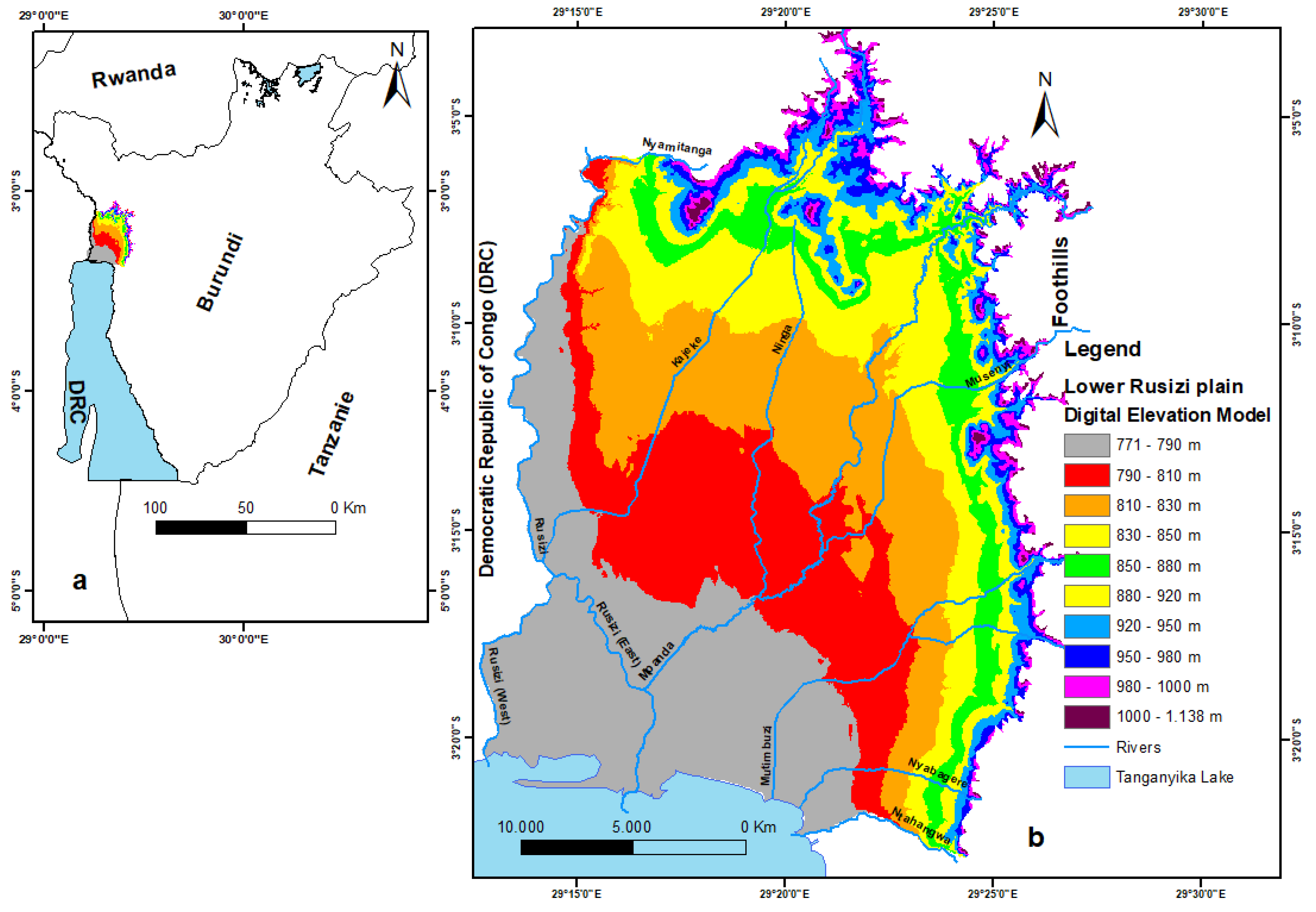
2.1.1. Location and Climate

The lower Rusizi plain is located in the northwest of Burundi (Figure 1) and covers about 632 km². This study area lies between southern latitudes of 3°03′00″ to 3°21′00″ and eastern longitudes of 29°12′00″ to 29°27′00″. Burundi has a tropical climate with some areas receiving a lot of rain, but others receiving less rain. In the lower Rusizi plain, the average annual rainfall varies from 800 to 850 millimeters, increasing strongly towards the foothills, where it can reach 1500 millimeters [1]. The distribution of rainfall during the year is characterized by the alternation of a dry season and a rainy season. The first rains usually arrive towards the end of September and stop normally at the end of May [2]. Like the rains, the temperatures vary according to the altitude [2]. The study area is among the warmest areas of Burundi with average annual temperatures above 23 °C [2]. The hydrographic network in the lower Rusizi plain consists of rivers which originate in the foothills and cross the plain from the northeast to the southwest, flowing either into the Rusizi River or directly into Lake Tanganyika.

2.1.2. Geological Setting

The geology of Burundi is subdivided into four large entities [4] including the Archean, which is the oldest and the least represented [5], the Burundian (middle Proterozoic) which covers most of the country hosting all the known mineralization indices in Burundi [6], the Malagarasian (Neoproterozoic) found in southeastern Burundi [7] and finally the Cenozoic represented by the tectonic rift deposits of Lake Tanganyika, consisting of lacustrine and fluvio-lacustrine alluvial deposits [8,9].

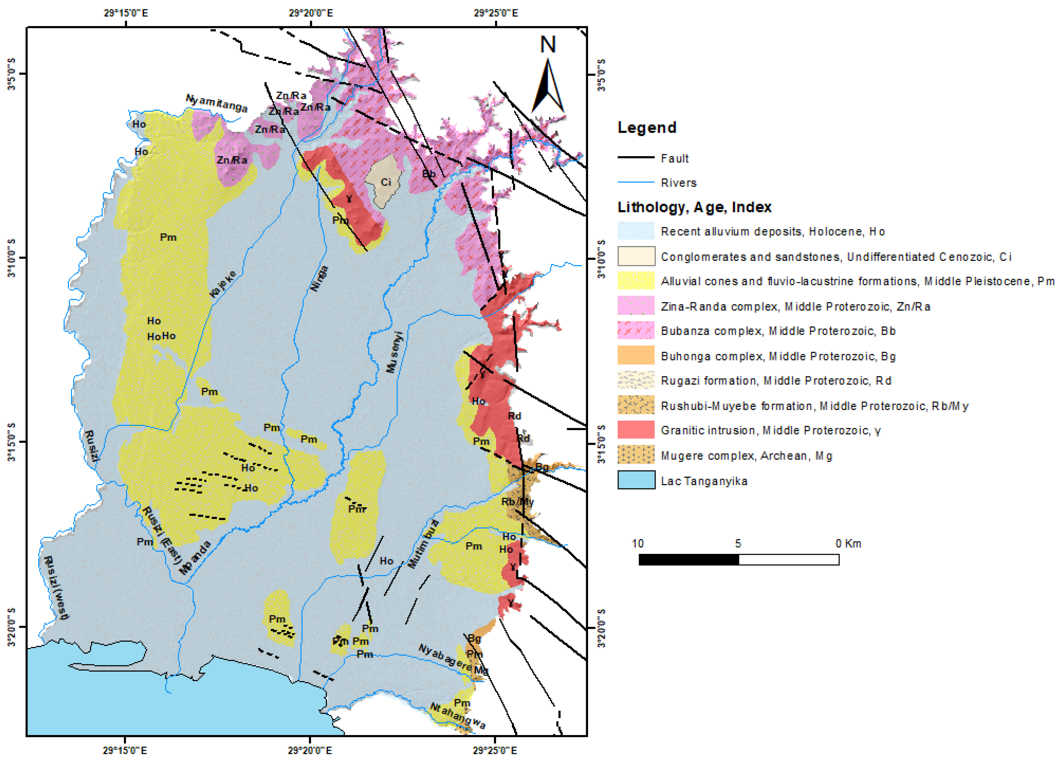
The lower Rusizi plain occupies the bottom of a large geological ditch which, like the northern ditch of Lake Tanganyika, would have resulted from a middle Pleistocene tectonic episode following an earlier episode to be related to the lower Pleistocene or older [1,2,3,4,5,6,7,8,9,10]. Geological formations are represented by a Precambrian set and a Cenozoic set (Figure 2). The Precambrian outcrops on the eastern border while the fluvio-lacustrine alluviums occupy the remainder of the area [11]. The western part of this plain is occupied by the recent alluvial deposits of the Rusizi (Holocene), while piedmont deposits from the foothills cover the eastern part [1]. Current alluvial deposits of several tributaries of Lake Tanganyika (Mutimbuzi) or Rusizi River (Mpanda, Kajeke) have been superimposed on the Middle Pleistocene fluvio-lacustrine alluvium [1,2,3,4,5,6,7,8,9,10,11,12].

Stratigraphically, we can distinguish, in the alluvial plain, Holocene, Middle Pleistocene, and undifferentiated Cenozoic formations [8] described in

Table 1. Stratigraphic description of the lower Rusizi plain.

Age	General Description
Holocene (Ho)	Essentially alluvial cone deposits developed at the foot of escarpments and deposits due to spreading runoff occupying a large part of the lower Rusizi plain, the recent alluvium of the Rusizi and its delta, as well as the beaches of Lake Tanganyika with coastal barriers mainly on the northern side.
Middle Pleistocene (Pm)	Represented by alluvial cones with flow-sheet flood sedimentary mechanisms and fluvio-lacustrine formations ranging from coarse sands to fine silt-clay deposits.
Undifferentiated Cenozoic (Ci)	Alluvial terraces and formations that consist of conglomerates and sandstone-quartzite rocks

.

Precambrian outcrops are located at the northern and eastern contacts between the plain and the foothills (Figure 2 and Figure 3). These Precambrian outcrops consist of middle Proterozoic magmatic and metamorphic formations [13] consisting of the complexes of Zina/Randa, Bubanza, and Buhonga, the Rushubi-Muyebe formation, and the granitic intrusions as shown in Figure 2. A small Archean outcrop is represented in the southeast of the plain and consists of the Mugere complex (Figure 2).

Figure 2. Geology of the study area (modified from the geological map of Burundi, Bujumbura sheet [14]).

Figure 2. Geology of the study area (modified from the geological map of Burundi, Bujumbura sheet [14]).

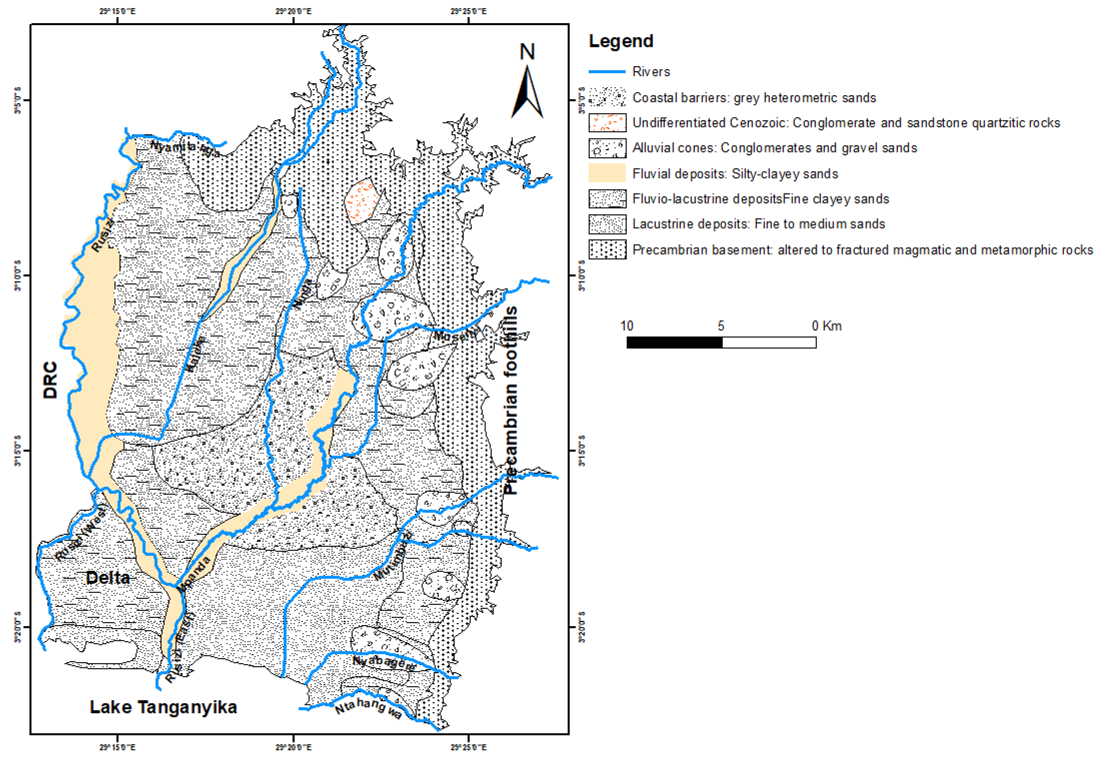
Therefore, the sedimentology of the lower Rusizi plain is represented by six facies [15] as shown in

Table 2. Sedimentological description of the Lower Rusizi Plain.

Facies	General Lithology
Lacustrine deposits	Fine to medium sand and mineralogical composition made by quartz, feldspar, and black minerals
Coastal barriers	Gray heterometric sands (quartz, feldspar, few micas, without black minerals), related to the combined action of lacustrine currents, waves, and wind. They are locally superimposed on lacustrine formations
Fluvial deposits	Silty-clay located along the Rusizi and its delta. To the east, they mix with lacustrine sediments, which are partly eroded by the rivers.
Fluvial deposits	Predominantly clayey, which develop to the northeast and east of the plain, in depressions with flat bottoms, limited on the western edge by slopes controlling the direction of the rivers.
Undifferentiated lacustrine and fluvial facies	Fine clayey sand, located between fluvial and lacustrine deposits
alluvial cone facies	Blocks and coarse sand to gravel, recognizable on the eastern side of the plain.

and Figure 3.

2.1.3. Hydrogeological Context

Two main drilling periods (1953–1960 and 2007–2015) have occurred in the considered area. During drilling, the depths of the first observed water inflow in the well were systematically recorded, inducing generally, a rise of the water level in the casing of the well [1,2,3]. This can be explained by noncontinuous lenticular layers of lower permeability within the aquifer inducing locally confined or partially confined conditions [1,2,3,4,5,6,7,8,9,10,11,12,13,14,15,16]. The depth to water measured in the wells, the total thickness of the aquifer, and the position of the lenticular clayey layers are variables. The thickness of the aquifer is relatively low in fluvial deposits (1 to 6 m) but is increased in littoral barriers and lacustrine deposits (more than 12 m).

The results from pumping tests were used to determine locally the hydrodynamic parameters, such as hydraulic conductivity values, which are used further in the calibration of the model. The lithological heterogeneity of the aquifer, as mapped in Figure 3, indicates that the hydrodynamic parameters calculated from the interpretation of pumping tests (in steady-state conditions and without monitoring piezometers) reflect local hydrogeological conditions around the corresponding wells. The hydraulic conductivities range from 10⁻⁶ and 2.2 × 10⁻² m/s.

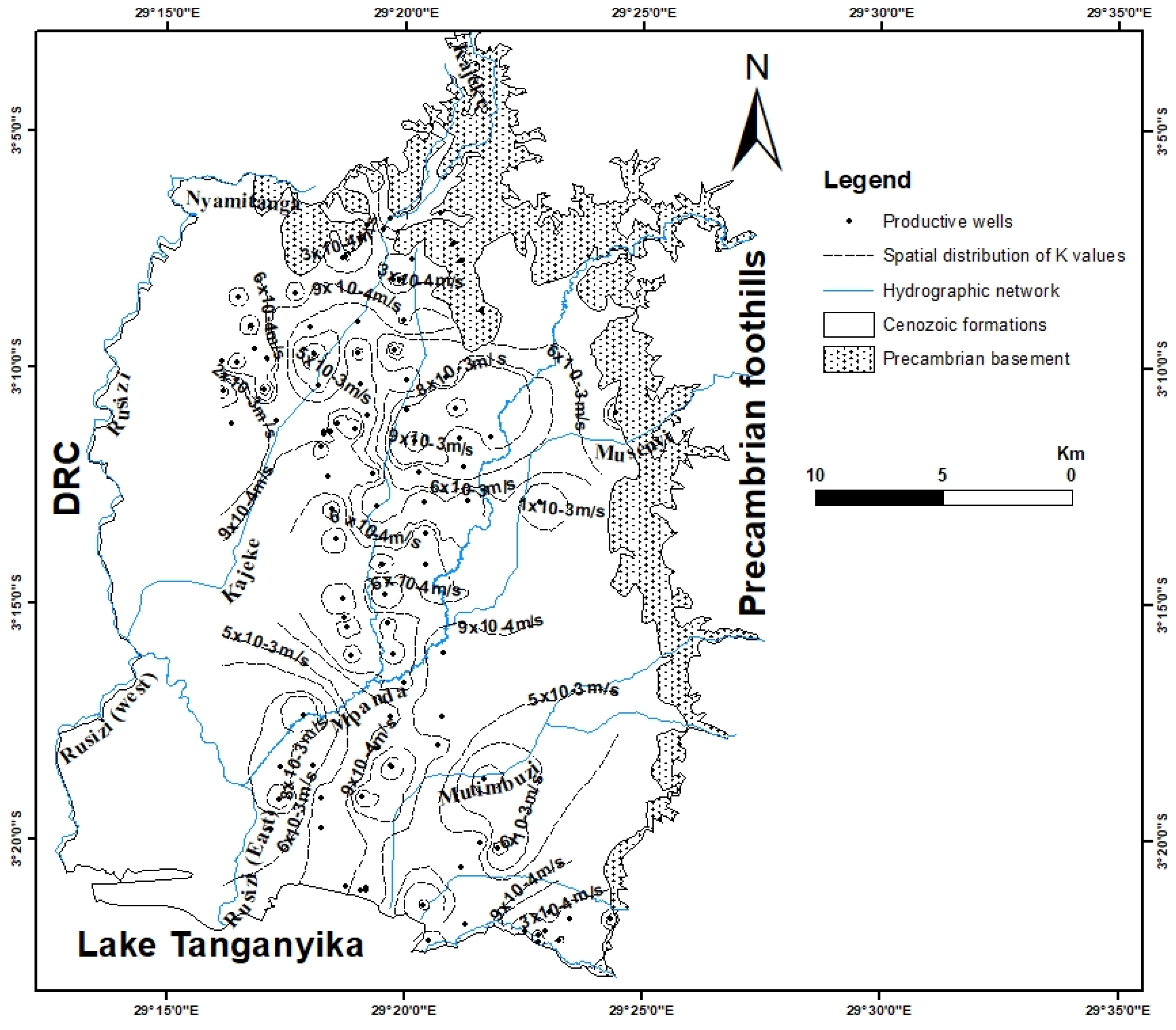
Even if the interpretation of the pumping tests cannot be generalized over the whole plain, a general trend in the spatial distribution of these hydraulic conductivity values can be observed (Figure 4). In general, hydraulic conductivity values decrease from south to north and from west to east and are generally low near the Precambrian foothills. However, this observation cannot be generalized in the alluvial cones investigated by the wells near the Kajeke and Mpanda rivers where hydraulic conductivity values range up to values of 1 × 10⁻³ m/s [3]. In the lacustrine deposits consisting of fine to medium sands, the hydraulic conductivity values vary between 9 × 10⁻⁴ and 9 × 10⁻³ m/s. Wells drilled within 300 m of the Lake Tanganyika shore had average hydraulic conductivity values ranging from 6 × 10⁻³ m/s to 9 × 10⁻⁴ m/s. In the coarse sand coastal barrier aquifer, the hydraulic conductivity values vary between 3 × 10⁻⁴ and 2.2 × 10⁻² m/s. In the fluvial deposits of the Rusizi River and its tributaries, the hydraulic conductivity values vary between 6 × 10⁻³ and 9 × 10⁻³ m/s. In the fluvio-lacustrine deposits consisting of fine clayey sand, the hydraulic conductivity values vary between 5 × 10⁻⁵ and 6 × 10⁻³ m/s. The wells that were drilled in the Precambrian basement present low hydraulic conductivity values around 1 × 10⁻⁶ m/s. The lowest values are found towards the eastern limit of the plain, while the highest values are found towards the southwest.

Figure 4 shows that in the lower Rusizi plain, some areas have not previously been investigated by any drilling. The model will thus provide an estimation of hydraulic conductivity values in those uninvestigated areas.

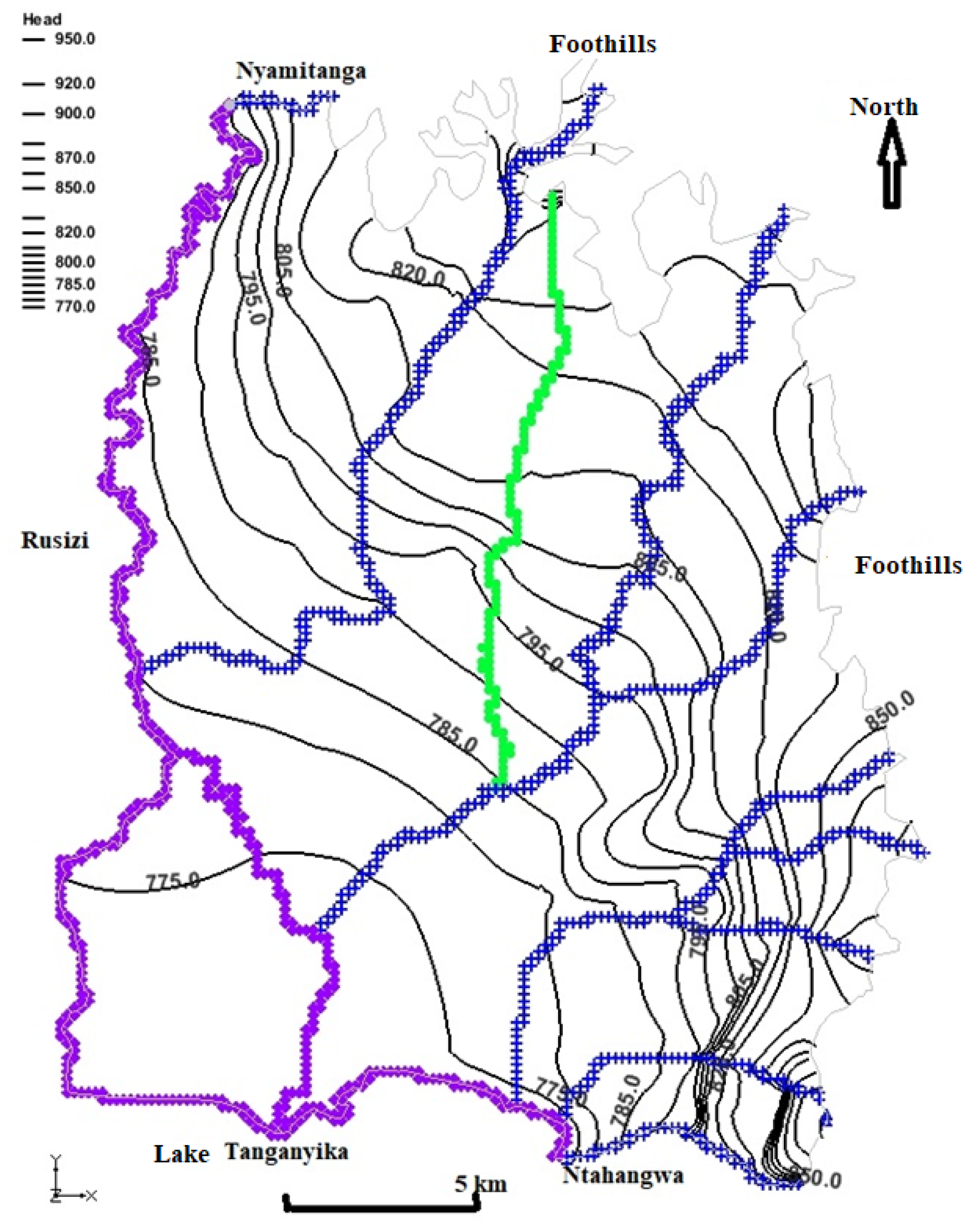
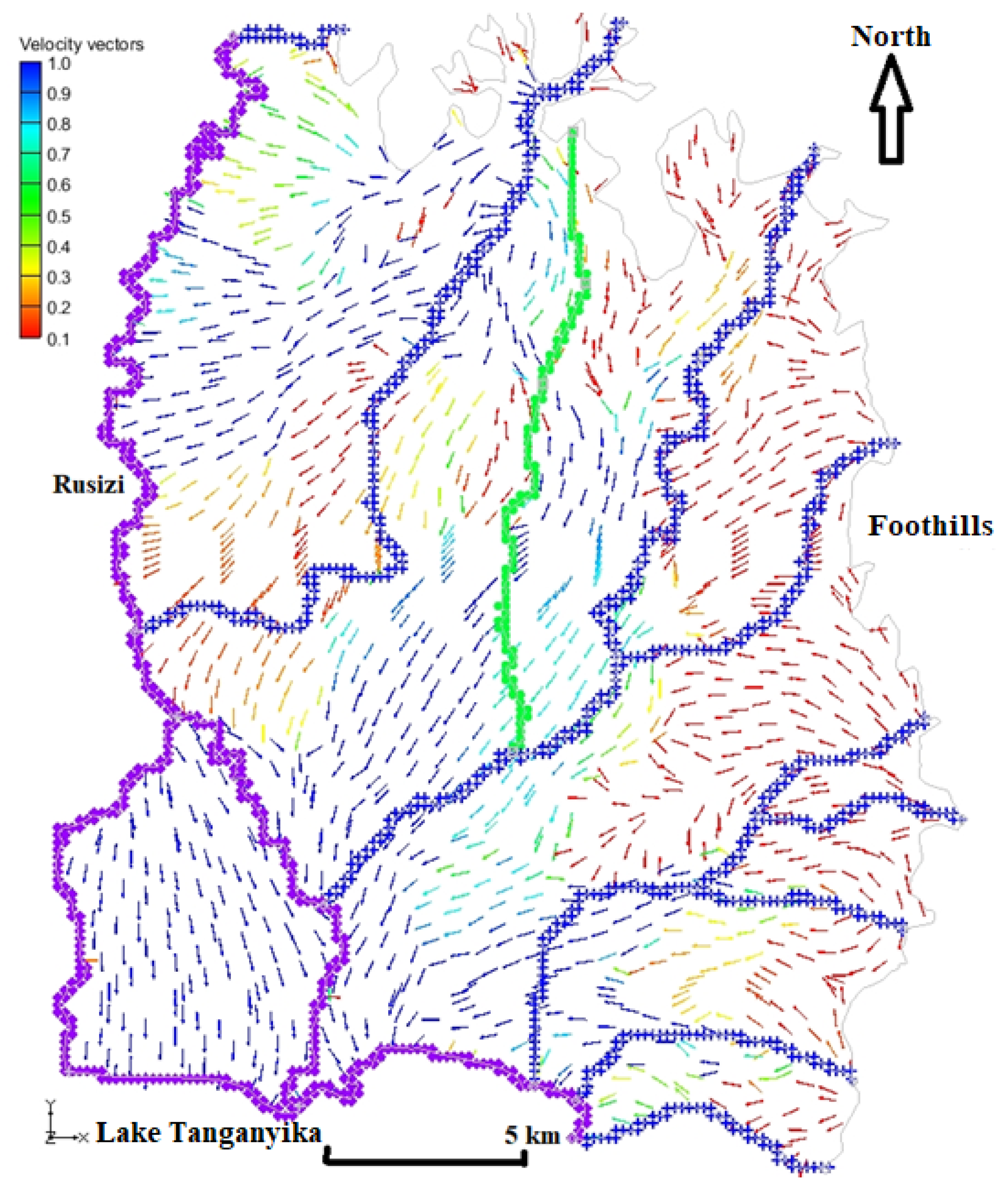
The reference piezometric map was established from the data of piezometric level measurements in the ancient drillings (1953–1960) [1,2] and has been updated with new data from drilling measurements that were carried out in the study area from 2007 to 2015 [3]. It reveals a general groundwater flow in the aquifer from the Precambrian basement located to the northeast and east of the plain, towards the southwest. The aquifer–river interactions are not similar from one river to another and from one area to another [3]. In the Kajeke river basin, the orientation of the potentiometric curves reflects the drainage of this river by the aquifer, while in the Mpanda river basin, the concavity of the potentiometric curves reflects drainage of the aquifer by this river. In other rivers, the orientation of the potentiometric line confirms that those rivers are drained by the aquifer. The concavity of the potentiometric lines oriented towards the East and North-East, except in the Mpanda river basin, also reflects a lateral recharge of the aquifer from the altered or fractured Precambrian formations. From an altitude between 795 m to 770 m, the potentiometric lines do not show a clear concavity and reflect a general balance between the river and the aquifer [3,4,5,6,7,8,9,10,11,12,13,14,15,16,17]. In contrast, at its western limit, this aquifer is drained by the Rusizi River and in the south, Lake Tanganyika constitutes its southern outlet.

The value of the hydraulic gradient varies from 0.3 in the southwest to 5% towards the southeastern limit, with an average value of 1.95% over the whole plain. In the southeast, between the Ntahangwa and Nyabagere rivers (Figure 5), the potentiometric curves are very tight, indicating low permeability, which is confirmed by the hydraulic conductivity values calculated in this area (10⁻⁴–10⁻⁵ m/s).

2.2. Groundwater Flow Modeling

A model is a simplified representation of a complex reality [18] or can be defined as a simplified version of a real system that approximately simulates the excitation–response relations of the latter [19]. For a typical groundwater flow model, the system to model is described by its geometry, its geological structures, and a whole set of hydraulic conductivity [18]. Stress factors can be recharge values or any pumping or reinjection flow rates [18]. Dependent variables are most often the spatially distributed piezometric heads in the domain [18]. The first step in the procedure of modeling is the construction of a conceptual model of the problem and the relevant aquifer domain [19]. A conceptual model represents how reality is simplified to be modeled [18] with an accepted set of assumptions [19]. The second step in modeling is to choose the mathematical model which consists here in expressing the volume groundwater conservation equation. This equation must be solved on the considered domain and its boundaries. The relevant state variable is the piezometric head. Initial conditions that describe the known state of the considered system at some initial time must be introduced, together with the boundary conditions that describe the interactions of the considered domain with its environment across these boundaries [19]. In the groundwater modeling process, calibration is a critical part [18] where the parameter values (here K-values) and their spatial distribution are adapted to obtain model results (piezometric heads) as close as possible to the observed values. After calibration, the model can be used for analyzing the prediction sensitivity to various scenarios of changes in stress factors [18].

The groundwater flow model of the lower Rusizi plain was constructed using Modflow 2005. This software is a finite difference model with block-centered nodes and this is the most widely used software for the calculation of steady-state or transient saturated groundwater flow [20,21].

2.2.1. Conceptual Model

The conceptual model provides a framework for designing, step-by-step, the numerical model [18,19,20,21,22]. Key components of a conceptual model include boundaries, hydrostratigraphy (i.e., stratigraphy based mostly on the hydraulic conductivity values), estimated values for the hydrogeological parameters, general directions of groundwater flow, sources and sinks of water, and a field-based groundwater budget [22].

Based on available data, only steady-state conditions could be considered for modeling the lower Rusizi plain aquifer. Due to the lack of vertically differentiated data in the alluvial sediments of the lower Rusizi plain, the model can be considered as 2D horizontal. The modeling assumptions are listed in

Table 3. Conditions and assumptions adopted for the development of the conceptual model.

Steady-state conditions corresponding to an averaged piezometry during the period 2007–2015;

Consolidation (land subsidence) is not considered;

The geological medium is porous and isotropic;

Darcy’s law is applicable;

The Dupuit assumption is considered (2D horizontal groundwater flow);

Water temperature is constant (isothermal conditions);

The aquifer is confined.

.

2.2.2. Boundary Conditions (BCs)

Boundary conditions are a key component of a mathematical model and may strongly influence the groundwater flow directions calculated by the model [22]. Boundaries can be used to represent hydraulic features, such as groundwater divides, and physical features, such as interactions with surface waters, lateral or vertical lithology changes implying relatively low permeability geological rocks [22].

The lower Rusizi plain 2D horizontal model is limited in the north, by the Palaeozoic foothills and the Nyamitanga river (Figure 5). Along the eastern boundary, the model is limited by the Paleozoic basement. In the south, the Ntahangwa river and the Lake Tanganyika constitute its southern boundary. In the west, it is limited by the Rusizi river and in the delta, the western branch of the Rusizi river (Figure 1) constitutes the western limit. The top and bottom of the model have been interpolated from the digital elevation model (DEM) taking into consideration the drilling log data. The piezometric levels were deduced from the depth to water measured in the wells before the pumping tests.

Three types of boundary conditions were chosen for the lateral boundaries. Based on the analysis of the spatial distribution of hydraulic conductivity values and the reference piezometric maps, the aquifer is considered as limited from the northeast to the southeast by the Precambrian basement. Those boundaries are thus considered impervious because the Precambrian basement is known as a low permeable bedrock. However, one can observe that the general groundwater flow of the aquifer is from northeast to southwest. All the fluxes entering the alluvial aquifer of the plain from the foothills are supposed to enter the model through the rivers which enter the plain by its eastern limit. To the south and the west, Lake Tanganyika and the Rusizi River constitute the southern and western outlets of the aquifer, respectively. Considering the situation described above, the boundary conditions were chosen as follows (Figure 6):

• Dirichlet BCs with prescribed piezometric heads at the southern boundary constituted by the Lake Tanganyika and the western boundary constituted by the Rusizi River;
• Neumann BCs as prescribed zero groundwater flux from the northeast to the southeast (the boundary with the Precambrian basement is considered as impermeable);
• Cauchy BCs describing river–aquifer interactions at the Ntahangwa and Nyamitanga rivers in the southern and northern boundaries respectively, at all rivers crossing the plain from the east to the west as well as the irrigation water collector Ninga (considered as a drain) (Figure 6) with conductance values to be part of the calibration procedure.

2.2.3. Stress Factors

The main stress factor in this model (top of the model) is constituted by recharge. The bottom of the model is considered to be impervious. Recharge was estimated from rainfall and temperature data recorded from two stations in the lower Rusizi plain over a 30-year period and two zones of recharge are considered (Figure 6). In the southern polygon, the average recharge was estimated at 83.9 mm/year, and in the northern part, it was estimated at 147.6 mm/year. The estimated average recharges represent 11% and 17% of the rainfall in the southern (40% of the whole study area) and northern parts (60% of the whole study area), respectively. This average recharge estimated over the model is 122.12 mm/year.

A large part of the lower Rusizi plain consists of rural villages, and rice and food crops except for the southern part in the urban area of Bujumbura. The majority of the wells that were drilled in this study area used manual groundwater pumps, except for the wells drilled in the industrial zone of Bujumbura and along the Lake Tanganyika beach. This is why we consider in this work that the Lower Rusizi plain aquifer is not strongly solicited by water extraction and that the pumped flow rates are considered as negligible to influence the piezometry at the entire plain scale.

2.2.4. Discretization

The available geological, hydrological and hydrogeological data allowed the discretization of the lower Rusizi plain aquifer by a horizontal 2D model with square cells of 200 m (Figure 7). The grid is oriented in the north–south (y-axis) and west–east (x-axis) directions with a total length of the x-axis = 25,970 m and a total length of the y-axis = 34,440 m. The total number of cells is 22,490.

2.2.5. Parameters

Hydraulic conductivity values were entered into the model distinguishing different zones in polygons on the basis of values obtained from the interpretation of the pumping tests as shown in

Table 4. Hydraulic conductivity values assigned to model polygons.

Polygon	K (m/s)	Polygon	K (m/s)	Polygon	K (m/s)	Polygon	K (m/s)
K1	0.0027	K16	0.001	K30	0.0001	K44	0.0028
K2	0.0021	K17	0.00021	K31	0.005	K45	0.0016
K3	0.0055	K18	0.00015	K32	0.00021	K46	0.0072
K4	0.000009	K19	0.0005	K33	0.000006	K47	0.0011
K5	0.00015	K20	0.0003	K34	0.0084	K48	0.0046
K6	0.00029	K21	0.00029	K35	0.0062	K49	0.00002
K7	0.00036	K22	0.00008	K36	0.000009	K50	0.0005
K8	0.00021	K23	0.000037	K37	0.00021	K51	0.0005
K9	0.00001	K24	0.00005	K38	0.00024	K52	0.003
K10	0.0061	K25	0.00024	K39	0.0016	K53	0.0075
K11	0.00014	K26	0.0046	K40	0.003	K54	0.0066
K12	0.00029	K27	0.0018	K41	0.002	K55	0.001
K13	0.000037	K28	0.00068	K42	0.0075	K56	0.0028
K14	0.0061	K29	0.0019	K43	0.00084	K57	0.00001
K15	0.0055					K58	0.0024

. A total of 58 polygons were created with an average hydraulic conductivity (K) value in each of them (Figure 8). Conductance values were also assigned to all river arcs with mixed boundary conditions. These are initial parameter values and an inverse model will be used to obtain a set of hydraulic conductivity and conductance values that minimize the calibration error.

3. Results

3.1. Model Calibration

The reference piezometry on which the model is calibrated corresponds to averaged piezometric level measurements taken in the most recent wells (2007–2015). From altitudes and the depth to water measured in each well, we obtained the piezometric levels (Figure 6) in 148 observation points. The highest piezometric level (949.12 m) was measured in the well located at the southeastern periphery of the plain towards the contact between the plain and the Precambrian basement. The mean level of Lake Tanganyika (771 m) is the lowest and constitutes the southern outlet of the aquifer.

Calibration was started with a trial-and-error and then automatic inverse modeling was completed using a parameter estimation (PEST) interface. The inverse model systematically adjusts a user-defined set of input parameters until the difference between the computed and observed values is minimized.

The groundwater flow model calibration was achieved (with a root mean square error (RMSE) of 4.38 m) through the automated parameter estimation method by adjusting hydraulic conductivity and conductance values. Sensitivity analysis shows that the model is strongly sensitive to hydraulic conductivity in the south and center of the plain, where hydraulic conductivity values used for reaching the calibration are higher than those estimated by the pumping test results. Figure 9 shows a comparison between computed and observed heads around the 1/1 line. The difference between computed and observed piezometric heads was generally less than 2 m in 114 wells and only in one well was a difference of more than 5 m observed.

The computed piezometric map (Figure 10) was close to the reference piezometry in areas where the piezometric levels have been measured and used for the development of the reference piezometric map (Figure 5). The computed piezometric levels calculated by the model allowed us to deduce the general groundwater flow directions of the aquifer in the areas not investigated through the recent drilling campaign.

3.2. Simulated Results

The model allowed for an estimation of the hydraulic conductivity values in different parts of the study area that were not explored by drilling until 2015. Indeed, the spatial distribution of the hydraulic conductivity values estimated by the model confirmed the heterogeneity of the aquifer in the lower Rusizi Plain.

Compared to the rest of the Lower Rusizi plain, from the northeast to the southeast, corresponding to the limit between the alluvial plain and the Precambrian basement, the hydraulic conductivity values are generally low and range around 9 × 10⁻⁶ m/s with an exception observed in polygon K50 (Figure 8) where the hydraulic conductivity value was estimated at 5 × 10⁻⁴ m/s (southeast). From the east to the west, the calibration of the model allowed the estimation of the following hydraulic conductivity values (Figure 8):

• In the fluvial deposits of the Mpanda river (polygons K23, K25, K35, K39, K41, K42, K42 in Figure 8), the hydraulic conductivity values increase from upstream to downstream by 3.7 × 10⁻⁵ m/s (K23) to 7.5 × 10⁻³ m/s (K42);
• In the fluvial deposits of the Kajeke river (polygons K11, K17, K16, K29, K30, K33, K32 in Figure 8), the hydraulic conductivity values are lower towards the downstream direction, 6 × 10⁻⁶ m/s (K33) and moderately high in the alluvial cones located near the contact between the alluvial plain and Precambrian basement, 3.6 × 10⁻⁴ m/s (K7);
• In the fluvial deposits of the direct tributaries of Lake Tanganyika, constituted by polygons K38, K57 and K58 (Figure 8), the hydraulic conductivity values vary between 10⁻⁵ and 2.4 × 10⁻⁴ m/s;
• In the Rusizi deposits, western limit, from the north (Nyamitanga river) to the south (polygons K1, K14 and K31 in Figure 8), the values of hydraulic conductivities vary between 2.7 × 10⁻³ and 6.2 × 10⁻³ m/s;
• In the fluvio-lacustrine deposits, the hydraulic conductivity values vary between 1.5 × 10⁻⁴ and 1.8 × 10⁻³ m/s;
• In the center of the plain, between the Kajeke and Mpanda rivers, there is a perimeter of coastal barriers represented by polygon K34, the hydraulic conductivity value estimated by the model is 8.3 × 10⁻³ m/s;
• In the Rusizi delta, the average hydraulic conductivity value estimated by the model is 8.4 × 10⁻⁴ m/s;
• In the lacustrine deposits, towards Lake Tanganyika, the hydraulic conductivity values estimated by the model vary between 2.8 × 10⁻³ and 7.5 × 10⁻³ m/s.

The groundwater flow directions were also visualized using the developed mathematical model. Logically, the main fluxes (blue color in Figure 11) were more concentrated in the areas of higher hydraulic conductivity values: in the littoral barriers, the lacustrine deposits, the alluvial cones of Kajeke river, and the fluvio-lacustrine deposits located in the Rusizi delta (Figure 11). The groundwater fluxes were lower (red color in Figure 11) towards the eastern boundary at the contact between the alluvial plain and the Precambrian basement where the hydraulic conductivity values remain low.

As discussed previously and shown on the reference piezometric map (Figure 5), the rivers that cross the plain from the East to the West are drained by the aquifer from their entrances in the alluvial plain except for the Mpanda river. Although the eastern limit is considered impermeable, important water fluxes enter the alluvial aquifer through the rivers. The model made it possible to estimate the water exchanges between the aquifer and the rivers that cross the plain from the east to the west. Table 4 illustrates aquifer–river interactions by estimation of the fluxes entering and leaving the aquifer for each river where mixed conditions were imposed during the calibration process. These exchanges or interactions between the aquifer and the rivers estimated by the model confirm the observed orientation of the piezometric lines (Figure 5) which illustrate the parts where the aquifer drains the rivers and those where the rivers drain the aquifer. It can be seen that in

Table 5. Optimized conductance (C) and computed flux (Q) through the different portions of the rivers represented within the model (+: aquifer drains river; −: river drains aquifer).

River	C (m2/s)	Computed Q m3/Day	River	C (m2/s)	Computed Q m3/Day
Nyamitanga	0.00012	+16,570	Murago	0.0000058	+2016
Kajeke	0.001	+273,162	Gikoma	0.00008	+39,727
Ninga	0.00038	0	Mutimbuzi	0.0000058	+4275
Mpanda	0.000015	−27,559	Nyabagere	0.0002	+82,945
Musenyi	0.0000058	+4793	Ntahangwa	0.00006	+57,419
Muzazi	0.00003	+16,642

, only the Mpanda River drains the aquifer from its entrance into the alluvial plain while the aquifer drains the Kajeke, Mutimbuzi, Nyabagere, and Ntahangwa rivers.

For limits with prescribed heads, the model computes the exchange fluxes between the aquifer and the Rusizi river on the one hand, and between the aquifer and the Lake Tanganyika on the other hand. The computed inflows and outflows for these boundaries are shown in

Table 6. Model outflows (−) and inflows (+) through the different portions of the Rusizi River and Lake Tanganyika represented in the model.

Type	Q m3/Day	Q m3/s
Rusizi (between Kajeke and Nyamitanga)	−536,879	−6.21
Rusizi (between Kajeke and delta)	7703	0.089
Rusizi (east of the delta)	−89,189	−1.03
Rusizi (west of the delta)	262,806	3.04
Tanganyika	−620,614	−7.18

. It can be observed that Lake Tanganyika and the Rusizi River (between Kajeke and Nyamitanga) are the boundaries where significant outflows are observed. At the western limit of the delta, water is entering the aquifer from the Democratic Republic of Congo (Figure 1) aquifer located on the other side of the river.

The groundwater budget was estimated using the zone budget package in Modflow. The groundwater balance for the entire study area is shown in

Table 7. Computed groundwater budget for the whole model of the lower Rusizi plain.

Source/Sink	Flow In (m3/Day)	Flow Out (m3/Day)
Constant head	993,377	−1,969,650
Drains	0	0
River leakage	821,606	−23,164
Recharge	177,809	0
Total source/sink	1,992,792	1,992,814

. It shows the boundaries where a significant quantity of water flows into the model and the boundaries where a significant volume of groundwater flows out of the model. By analyzing Table 7, we can observe that at the prescribed piezometric head boundaries, the volumes of water entering into the model represent less than half of the outflows from the model. These outflows are then balanced by direct recharge and interaction between the aquifer and the rivers that cross the plain from east to west.

4. Discussion and Conclusions

The developed model is a way to integrate all the previously collected, measured, and interpreted data into one single tool that is very useful for understanding and selecting priorities for future measurements, predicting future scenarios such as the climate effect on groundwater resources, and to prevent the excessive use of groundwater.

The results of this model allowed us to establish a computed piezometric map of the entire study area and also to estimate the hydraulic conductivity values in areas that have never been investigated by drilling. The orientation of the piezometric contours and groundwater budget allowed us to observe the river–aquifer interactions. The associated spatial distribution of the hydraulic conductivity values that were introduced into the model for calibration shows that the lower Rusizi aquifer is highly heterogeneous as expected from the Precambrian basement (east), where the values are around 1 × 10⁻⁶ m/s, to the southwestern areas in the lacustrine deposits and coastal barriers, where they are around 7.5 × 10⁻³ m/s. This heterogeneity due to the spatial distribution of hydraulic conductivity values allows us to identify areas with high groundwater potential, such as the coastal barriers, lacustrine deposits, alluvial cones and fluvio-lacustrine formations located in the western part of the study area. This model also allowed us to estimate the quantity of water entering and leaving the lower Rusizi plain aquifer by the prescribed piezometric head boundaries constituted by the Rusizi River and Tanganyika Lake, respectively, in the western and southern limits. It can be seen that the outflows are slightly higher than the inflows, whereas the aquifer is not extensively used. The increased use of groundwater in the lower Rusizi plain may create an unbalanced situation between inflows and outflows in the future, which would have serious consequences on the availability of this resource.

Long duration pumping tests with drawdown measurements in the monitoring piezometers, piezometric level measurement campaigns over different periods of the year and the installation of a network of piezometers in the Lower Rusizi plain could contribute to the determination of specific yield values and the monitoring of piezometric level fluctuations that are needed for further transient monitoring and modeling of this aquifer.

This mathematical flow model that has been calibrated in representative steady-state conditions will be the basis for a future groundwater management tool that will be developed in transient conditions. The progressive and periodic introduction of updated piezometric levels into the model for the sake of transient calibration and validation will allow us to obtain a reliable tool to simulate the hydrodynamic behavior of the aquifer in the lower Rusizi plain.

The developed model will be a predictive tool and will contribute to the resolution of problems related to the use and integrated management of the groundwater resource in this part of Burundi.

This model can already be used for prediction purposes and consequently can serve for studying different development plans of the Rusizi plain, involving the development of the drinking water supply and the extension of residential, agricultural and industrial areas.

References

1. Waleffe, A. Esquisse hydrogéologique de la plaine de la basse Rusizi (Burundi). Dép. Géol. Miner. Rap. Annu. 1985, 1983–1984, 177–187. [Google Scholar]
2. Hakiza, G. Potentialités Aquifères de la Plaine de la Rusizi (au Nord du lac Tanganyika). Ph.D. Thesis, University of Liège, Liège, Belgium, 2002. [Google Scholar]
3. Ngenzebuhoro, P.C.; Mohammed, S.; Bahaj, T.; Faouzi, M.; Kacimi, I. Géométrie et caractérisation hydrodynamique d’un système aquifère plio-quaternaire; Cas de la plaine de la basse Rusizi (Burundi). Bull. L’institut Sci. Sect. Sci. Terre 2019, 37–53. [Google Scholar]
4. Ntungicimpaye, A. Contribution à L’Étude du Magmatisme Basique dans le Kibarien de la Partie Occidentale du Burundi. Ph.D. Thesis, Ghent University, Ghent, Belgium, 1984. [Google Scholar]
5. Tack, L.; Liégeois, J.P.; Deblond, A.; Duchesne, J.C. Kibaran A-type granitoids and mafic rocks generated by two mantle sources in a late orogenic setting (Burundi). Precambrian Res. 1994, 68, 323–356. [Google Scholar] [CrossRef]
6. Klerkx, J.; Liégeois, J.-P.; Lavreau, J.; Claessens, W. Crustal evolution of the northern Kibaran belt, eastern and central Africa. Proterozic Lithospheric Evol. 1987, 17, 217–233. [Google Scholar]
7. Tack, L. The Neoproterozoic Malagarazi supergroup of SE Burundi and its equivalent Bukoban System in NW Tanzania: A current review. In Annales-Musée Royal de L’Afrique Centrale Série in 8vo Sciences Géologiques; Royal Museum of Central Africa: Tervuren, Belgium, 1995; pp. 121–130. [Google Scholar]
8. Ilunga, L. Le Quaternaire de la Plaine de la Ruzizi. Etude Morphologique et Lithostratigraphique. Ph.D. Thesis, Vrije Universiteit, Bruxelles, Belgium, 1984. [Google Scholar]
9. Ilunga, L. Morphologie, volcanisme et sédimentation dans le rift du Sud-Kivu. Bull. Soc. Géograph. Liège 1991, 27, 209–228. [Google Scholar]
10. Cahen, L. Géologie du Congo Belge, 1st ed.; H. Vaillant-Carmanne: Liège, Belgium, 1954; pp. 17–34. [Google Scholar]
11. Ilunga, L. Environnements Sédimentaires et Minéralogie des Formations Superficielles de la Plaine de la Ruzizi (Nord du Lac Tanganyika). Geo-Eco-Trop 2007, 31, 71–104. [Google Scholar]
12. Frankart, R.P.; Herbillon, A.J. Aspects de la Pédogenèse des Sols Halomorphes de la Basse Rusizi, Burundi, 1st ed; Musée Royal de L’Afrique Centrale: Tervuren, Belgium, 1971; pp. 83–96. [Google Scholar]
13. Theunissen, K. On the Rusizian basement rise in the Kibara belt of Northeastern Lake Tanganyika. Collision belt geometry or restraining bend emplaced in the Late Kibaran strike-slip environment. IGCP Newsl. 1989, 2, 85–92. [Google Scholar]
14. Theunissen, K. Carte Géologique du Burundi—Feuille Bujumbura. Musée Royal de l’Afrique Centrale (Tervuren, B., Département de Géologie et de Minéralogie, Burundi, & Ministère des Travaux Publics, de L’énergie et des Mines. S4/29-N.W, S4/29-N.W. 1989. Available online: https://www.sudoc.fr/115386793 (accessed on 21 October 2021).
15. Chorowicz, J.; Thouin, C. Failles synsédimentaires et structure de la plaine de la Rusizi (Nord-Tanganyika). C. R. L’académie Sci. Sér. 2 Méc. Phys. Chim. Sci. L’univers Sci. Terre 1985, 301, 835–840. [Google Scholar]
16. Snel, M.J. Contribution à L’étude Hydrogéologique du Congo Belge, 4th ed; Direction Générale Du Service Géologique—Congo Belge: Brussels, Belgium, 1957; Volume 2, pp. 26–29. [Google Scholar]
17. De Marsily, G. Quantitative Hydrogeology: Groundwater Hydrology for Engineers, 1st ed.; Orlando, F.L., Ed.; Academic Press: Cambridge, MA, USA, 1986; pp. 329–387. [Google Scholar]
18. Dassargues, A. Hydrogeology-Groundwater Science and Engineering; Taylor & Francis CRC Press: Boca Raton, FL, USA, 2018; pp. 345–395. [Google Scholar]
19. Bear, J.; Verruijt, A. Theory and Applications of Transport in Porous Media. In Modeling of Groundwater Flow and Pollution, 1st ed.; D. Reidel Publishing Company: Dordrecht, The Netherlands, 1987; pp. 53–114. [Google Scholar]
20. Mondal, N.C.; Singh, V.S. Mass transport modeling of an industrial belt using visual MODFLOW and MODPATH: A case study. J. Geogr. Reg. Plan. 2009, 2, 001–019. [Google Scholar]
21. Surinaidu, L.; Gurunadha Rao, V.V.S.; Srinivasa Rao, N.; Srinu, S. Hydrogeological and groundwater modeling studies to estimate the groundwater inflows into the coal Mines at different mine development stages using MODFLOW, Andhra Pradesh, India. Water Resour. Ind. 2014, 7–8, 49–65. [Google Scholar] [CrossRef] [Green Version]
22. Anderson, M.P.; Woessner, W.W.; Hunt, R.J. Applied Groundwater Modeling: Simulation of Flow and Advective Transport, 2nd ed; Academic Press: San Diego, CA, USA, 2015; pp. 115–249. [Google Scholar]
Figure 1. (a) Location map of the study area in Burundi; (b) limits of the lower Rusizi plain on the digital elevation model (10 m resolution) and presentation of the hydrographic network crossing the plain from the northeast to the southwest.
Water 13 03376 g001
Figure 3. Sedimentological sketch of the aquifer in the lower Rusizi plain.
Water 13 03376 g003
Figure 4. Map showing the location of drilling and spatial distribution of hydraulic conductivities values in the lower Rusizi plain [3].
Water 13 03376 g004
Figure 5. Reference piezometric map of the lower Rusizi plain.
Water 13 03376 g005
Figure 6. Map showing the two recharge polygons used to estimate the average recharge over the entire lower Rusizi plain.
Water 13 03376 g006
Figure 7. Boundary conditions and model discretization.
Water 13 03376 g007
Figure 8. Spatial distribution of the hydraulic conductivity polygons introduced in the model.
Water 13 03376 g008
Figure 9. Comparison of computed and observed piezometric heads after the calibration of the steady-state groundwater flow model.
Water 13 03376 g009
Figure 10. Computed piezometric map.
Water 13 03376 g010
Figure 11. Map showing the computed intensity of the groundwater flux vectors.
Water 13 03376 g011