Article

Spatiotemporal Landslide Susceptibility Mapping Incorporating the Effects of Heavy Rainfall: A Case Study of the Heavy Rainfall in August 2021 in Kitakyushu, Fukuoka, Japan

1
School of Civil Engineering, Central South University, Changsha 410075, China
2
MOE Key Laboratory of Engineering Structures of Heavy-Haul Railway, Central South University, Changsha 410075, China
3
State Key Laboratory of Geohazard Prevention and Geo-Environment Protection, Chengdu University of Technology, Chengdu 610000, China
4
Department of Civil Engineering, Kyushu University, Fukuoka 819-0395, Japan
*
Author to whom correspondence should be addressed.
Water 2021, 13(22), 3312; https://doi.org/10.3390/w13223312
Submission received: 3 November 2021 / Revised: 18 November 2021 / Accepted: 19 November 2021 / Published: 22 November 2021
(This article belongs to the Special Issue Remote Sensing and GIS for Geological Hazards Assessment)

Abstract

:
Landslide represents an increasing menace causing huge casualties and economic losses, and rainfall is a predominant factor inducing landslides. Landslide susceptibility assessment (LSA) is a commonly used and effective method to prevent landslide risk, however, the LSA does not analyze the impact of the rainfall on landslides which is significant and non-negligible. Therefore, the spatiotemporal LSA considering the inducing effect of rainfall is proposed to improve accuracy and applicability. In this study, the influencing factors are selected using the chi-square test, out-of-bag error and multicollinearity test. The spatial LSA are thus obtained using the random forest (RF) model, deep belief networks model and support vector machine, and compared using receiver operating characteristic curve and seed cell area index to determine the optimal assessment result. According to the heavy rainfall characteristics in the study area, the rainfall period is divided into four stages, and the effective rainfall model is employed to generate the rainfall impact (RI) maps of the four stages. The spatiotemporal LSAs are obtained by coupling the optimal spatial LSA and various RI maps and verified using the landslide warning map. The results demonstrate that the optimal spatiotemporal LSA is obtained using the spatial LSA of the RF model and temporal LSA of the rainfall data in the peak stage. It can predict the area where rainfall-induced landslides are likely to occur and prevent landslide risk.

1. Introduction

Landslides are one of the most common geo-hazards on Earth and result in considerable damage to life and property [1,2]. It is critical to accurately evaluate landslide-prone areas to effectively determine the locations and times of landslides [3]. Landslide susceptibility assessment (LSA) is thus an effective risk management measure to prevent landslides and reduce landslide risk [4].
Rainfall-induced landslides are a typical cascading geo-hazard and are attracting the increasing attention of many researchers [5,6]. Rainfall-induced landslides commonly occur after heavy rainfall and may develop into potentially catastrophic movements [7,8]. Heavy rainfall or prolonged rainfall may result in the increase of pore-water pressure and the significant decrease of friction force, which causes slope instability [9,10,11]. Hence, in addition to analyzing the spatial LSA using the environmental condition factors, it is also necessary to analyze the temporal LSA using the rainfall data to illustrate the impact of heavy rainfall on landslides, which ensures the availability and accuracy of LSA [12,13,14]. Spatiotemporal landslide susceptibility mapping (LSM) is thus studied as an excellent method of susceptibility assessment and provides information on potential landslides under the impact of heavy rainfall [15,16].
The analysis of spatial LSA generally assumes that future landslides are more likely to occur in similar environmental conditions to previous landslides [17]. The LSA thus can predict the potential risk areas using the historical landslide data and environmental condition factors [18]. The selection of influencing factors is an essential part of LSA, and most current research selects the influencing factors using correlation test and multicollinearity test to prove the correlation between influencing factors and landslides and avoid a redundancy of influencing factors [19,20,21].
Meanwhile, the LSA results are affected by evaluation models, and it is very important to select the appropriate models for LSA [22,23,24]. There are various models to analyze the LSA, and these are generally classification models [25]. Early studies map the landslide susceptibility using traditional statistical analysis models, such as linear discriminant analysis, weights of evidence, frequency ratio models and regression models [26,27,28,29]. Most current studies propose various machine learning algorithms, such as support vector machines (SVM), naive Bayesian model, random forest (RF) models, and artificial neural networks, to evaluate the landslide susceptibility [28,30,31,32,33]. Because of the complex environmental conditional factors of landslides in study areas, the accuracy and applicability of LSA obtained using various models are very different. It is thus essential to select the evaluation models that are more applicable to the study area.
On the other hand, rainfall is one of the most critical inducing factors, especially heavy and prolonged rainfall, and rainfall analysis is thus one of the core steps in the temporal LSA [34,35]. The impact of rainfall intensity and duration on landslides has long been an issue of great interest for researchers in LSA [36,37]. The effective rainfall model (ERM) is a common and effective method and employs the rainfall data of some days before the study time to indicate the impact of rainfall, which can illustrate the temporal landslide susceptibility of the study area [38,39].
The present study proposes a methodology to evaluate spatiotemporal landslide susceptibility incorporating the effects of heavy rainfall, and the methodology is applied to the Kitakyushu, Fukuoka, Japan. Multi-source data such as the condition factors, historical landslides, heavy rainfall data and landslide warning map are considered. In the spatial LSA, the chi-square ( χ 2 ) test, out-of-bag (OOB) error and multicollinearity test are employed to select the influencing factors, and the spatial LSMs are thus obtained using the RF model, deep belief networks (DBN) model and SVM model. The accuracies of the spatial LSMs are proved using receiver operating characteristic (ROC) curve and seed cell area index (SCAI) to obtain the optimal spatial LSM used for spatiotemporal LSM. Based on the heavy rainfall data in August of the study area, the heavy rainfall period is divided into four stages, and the rainfall impact (RI) maps of the four stages are thus generated using ERM. The spatiotemporal LSMs are obtained by coupling the optimal spatial LSM and temporal LSMs and verified using the landslide warning map to determine the optimal spatiotemporal LSM, which provides a reference for landslide prevention.

2. Materials and Methods

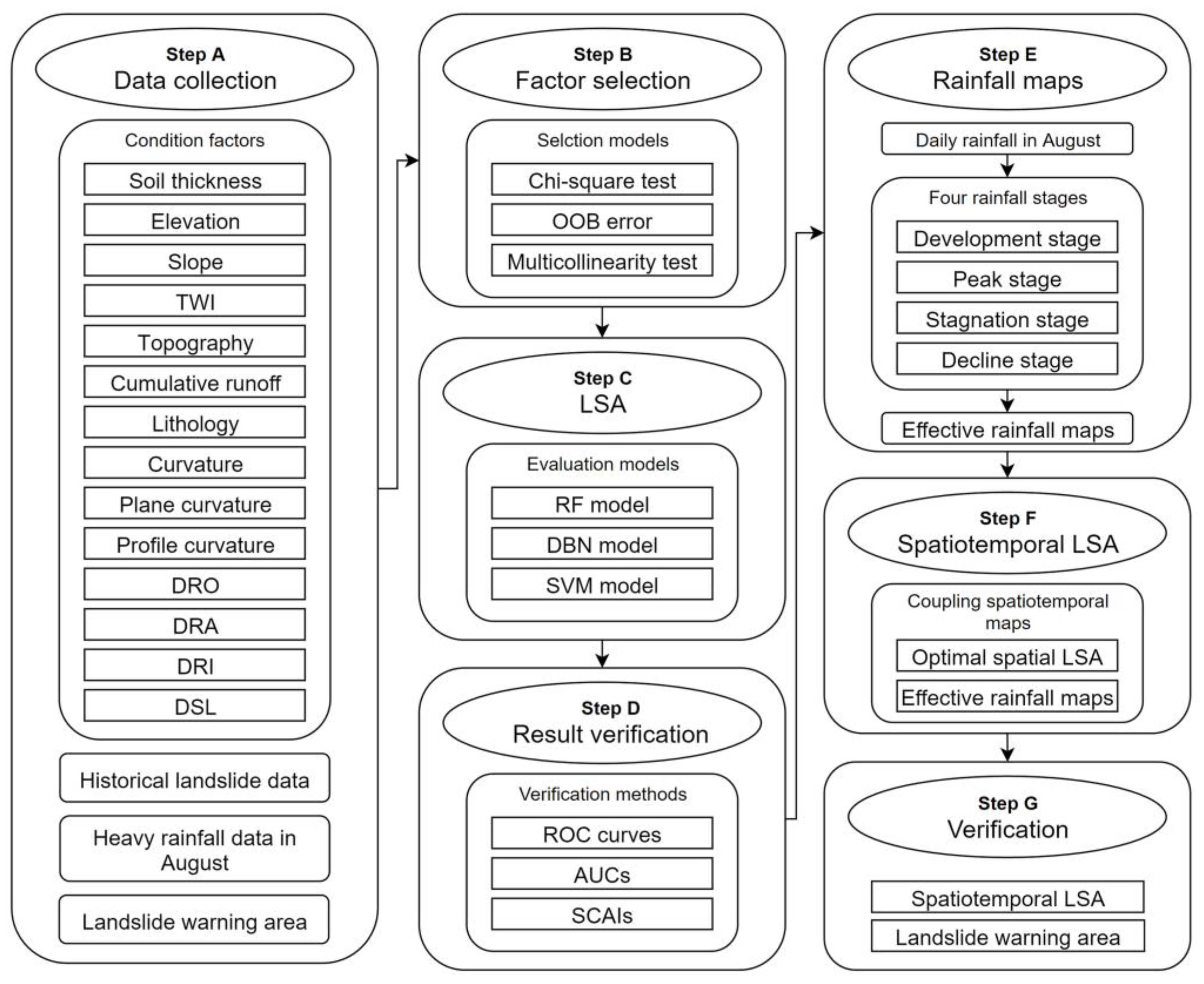
2.1. Methodological Flow

The steps and processes of the LSM procedures involved in the present study (Figure 1) are as follows:
The methodology framework of the proposed LSM can be divided into seven steps: (a) data collection: the data of various condition factors of landslides and the historical landslides are collected, and heavy rainfall data in August and landslide warning map are prepared. (b) Influencing factor selection: the influencing factors are selected as the LSA indices using the χ 2 test, OOB error and multicollinearity test. (c) LSA: the LSMs are obtained using the RF model, DBN model and SVM model. (d) Result verification: the results of LSA are verified using ROC curve, area under the curve (AUC) and SCAI to determine the optimal spatial LSA. (e) Rainfall map generation: the heavy rainfall period in the study area is divided into four stages, namely the development stage, peak stage, stagnation stage and decline stage, and the rainfall maps of various stages are generated using the interpolation method, and the RI maps of various stages are obtained and normalized by the effective rainfall model. (f) Spatiotemporal LSA: various RI maps are coupled with the optimal spatial assessment result to obtain the spatiotemporal susceptibility maps under the influence of heavy rainfall in August. (g) Spatiotemporal assessment verification: the various spatiotemporal LSMs are verified using the landslide warning map to determine the optimal spatiotemporal LSM.

2.2. Factor Selection Methods

The χ 2 test is one of the most common methods to determine the correlation between influencing factors and landslides, and the variance inflation factor (VIF) is a commonly used index to test multicollinearity which refers to the linear correlation between independent variables [19,20,21]. The χ 2 test determines the accuracy of the hypothesis by calculating the deviation of the actual value from the theoretical value, and the χ 2 can be obtained using Equation (1). The hypothesis is verified by comparing the χ 2 with the critical value of a significance test.
χ 2 = i = 1 n ( A i T ) 2 T ,
where A i is the i t h actual value and T is the theoretical value.
Multicollinearity of influencing factors is verified using VIF. The smaller the VIF value, the less significant the multicollinearity, and the greater the VIF value, the more significant the multicollinearity. The VIF value is thus closer to 10 indicating stronger multicollinearity between the influencing factors [26,40,41]. The VIF can be obtained using Equation (2).
V I F = 1 1 R i 2 ,
where R i is the correlation coefficient of the i t h independent variable to other independent variables.
The OOB error is a widely employed method to select the influencing factors and determine their significance. The OOB error is calculated using the ratio of misclassification number to the total number. In the present study, based on the recursive feature elimination (RFE), the OOB error is thus used to eliminate the factor with the least importance using variable importance measures (VIM) and to determine the optimal number of landslide influencing factors [42].

2.3. Landslide Susceptibility Assessment (LSA) Methods

The RF model and SVM model are currently commonly used models [28,31], while the DBN model is a relatively novel model used for the LSA [43]. The applicability of the three models for the LSA is proved, and the present study thus selects the three models, namely the RF model, DBN model and SVM model to analyze the LSA.

2.3.1. Random Forest (RF) Model

The RF model was proposed as an advanced integrated learning algorithm using the ensemble of unpruned classification trees in 1995. It is a classifier training samples by multiple trees [44,45]. The trees are constructed according to the following four steps: (a) N denotes the number of training samples, while M denotes the number of characteristics. (b) The number of characteristics is inputted to determine the decision result of the previous node on the decision tree. (c) The training set is generated using the bootstrap sampling method, and the unselected samples are used to predict and evaluate the errors. (d) The characteristics are selected randomly to determine the decision of each node on the decision tree, and the optimal splitting method is calculated [46].

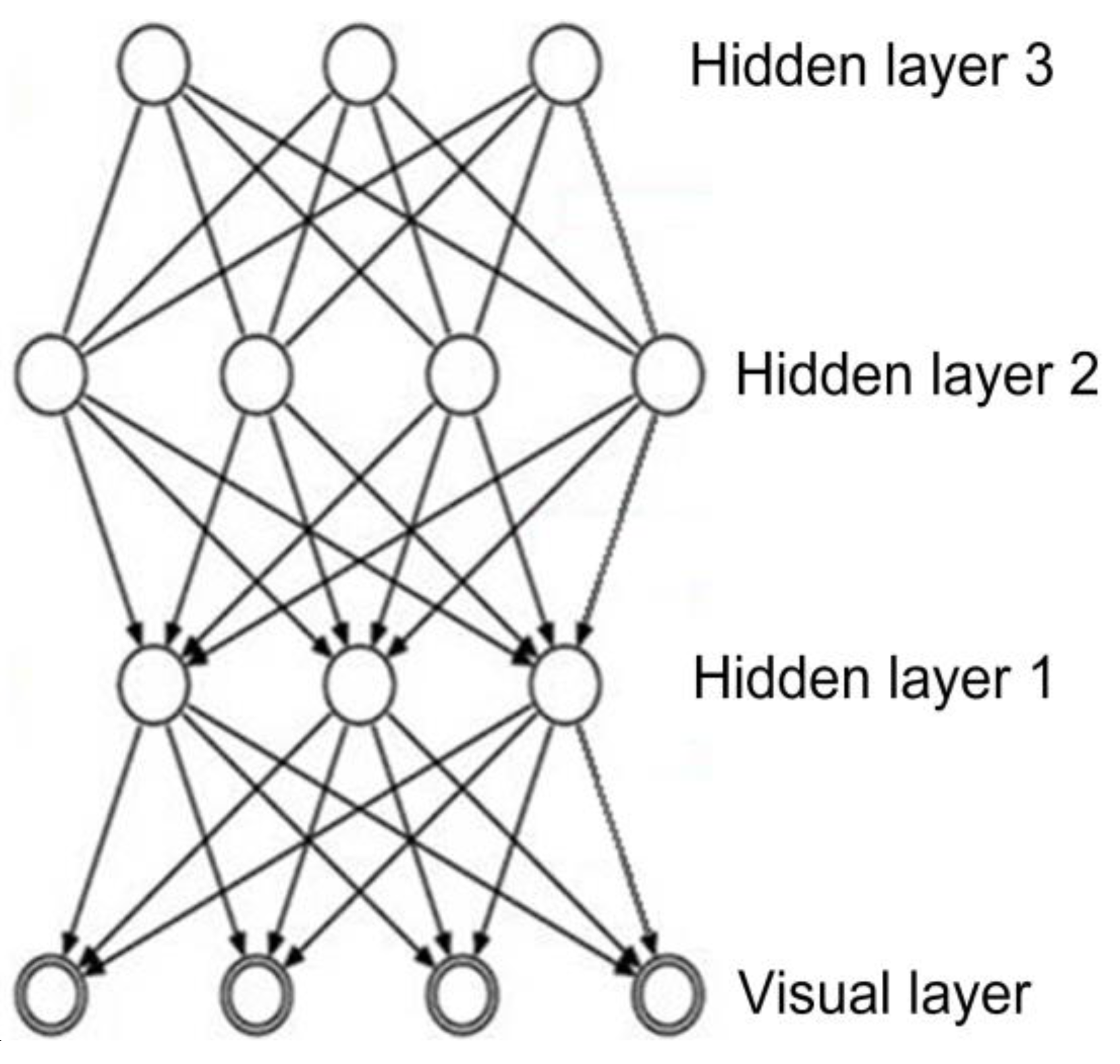
2.3.2. Deep Belief Networks (DBN) Model

The DBN model is an efficient unsupervised learning algorithm and is also a probabilistic generative model [47]. Compared with the traditional neural network, it generates a joint distribution between the observation data and the label. The DBN model is composed of restricted Boltzmann machines (RBM) which consists of the visual layer υ and hidden layer h . There is no connection between the neurons in a layer, while there are connections between layers, and every layer can be considered as a logistic regression model. The hierarchical structure is very close to the structure of the human brain. Several RBMs structure a DBN, and the hidden layer of the previous RBM is the visual layer of the current RBM. The structure of the DBN model is presented in Figure 2.
In RBM, each neuron has a bias coefficient b for visual neuron and c for hidden neuron, and the weight W between two connected neurons is the connection weight. The energy of the RBM can be obtained using Equation (3).
E ( υ , h ) = i = 1 N υ b i υ i j = 1 N h c j h j i , j = 1 N υ , N h W i j υ i h j ,
where N υ is the number of visual neurons; N h is the number of hidden neurons.

2.3.3. Support Vector Machines (SVM) Model

The SVM model is a classifier developed from the generalized portrait algorithm in pattern recognition. It can be used for classification, regression and outlier detection based on the principle of minimizing statistical and structural risk. The sample data are normalized and mapped using kernel functions to build the SVM model, and the hyperparameters of the SVM model are optimized to train the model. The SVM model can be performed using various kernel functions, such as linear kernel (Equation (5)), polynomial kernel (Equation (6)), radial basis function kernel (Equation (7)) and sigmoid kernel (Equation (8)). The main control hyperparameters are the penalty parameter and kernel function parameter. The penalty parameter is introduced, and the objective function can be obtained using Equation (4):
f ( x ) = m i n 1 2 w 2 + C i = 1 n ξ i ,
where 1 2 w 2 is the geometric interval; C is the penalty parameter; and ξ i is the slack variable. And the various kernel functions can be obtained using Equations (5)–(8):
K ( x i , x ) = x i · x ,
K ( x i , x ) = [ ( x i · x ) + 1 ] m ,
K ( x i , x ) = exp ( x i x , 2 2 δ 2 ) ,
K ( x i , x ) = tan h ( η < x i , x > + θ ) .

2.4. Effective Rainfall Model (ERM)

The ERM reflects the rainfall accumulation that stays in the rock and contributes to the development of landslides. The model was proposed by Kohler and Linsley in 1951 as an antecedent precipitation index to predict the surface runoff based on hydrological data [48]. The effective rainfall can be obtained using Equation (9).
R e = i = 0 n K i R i ,
where K is the attenuation coefficient and considered as 0.8; and R i is the rainfall of the previous i t h day.
In the present study, the rainfall data are collected from meteorological observation stations in the study area. The maps of rainfall during the study time are thus generated using the kriging interpolation method, and the effective rainfall map can be obtained using the ERM.

2.5. Validation Methods

Verifying the accuracy of susceptibility assessment results obtained using various models is a key task of susceptibility research. In the present study, the SCAI and ROC curve methods were selected to verify the accuracy of susceptibility assessment. The SCAI can be obtained using Equation (10).
S C A I = P i P i ,
where P i is the areal percentage of the susceptibility level i ; and P i is the areal percentage of the landslides at level i .
The ROC curve is a commonly used method to verify the accuracy of assessment results [49]. The ROC curve was obtained using two variables, namely the specificity and sensitivity. The variables can be obtained using Equations (11) and (12):
S p e c i f i c i t y = T N F P + T N ,
S e n s i t i v i t y = T P T P + F N ,
where F P is the false positive; T N is the true negative; T P is the true positive; and F N is the false negative.
The threshold for AUC values is 0.5 to 1, and the closer it is to 1, the more accurate the model is [50].

3. Study Area and Dataset
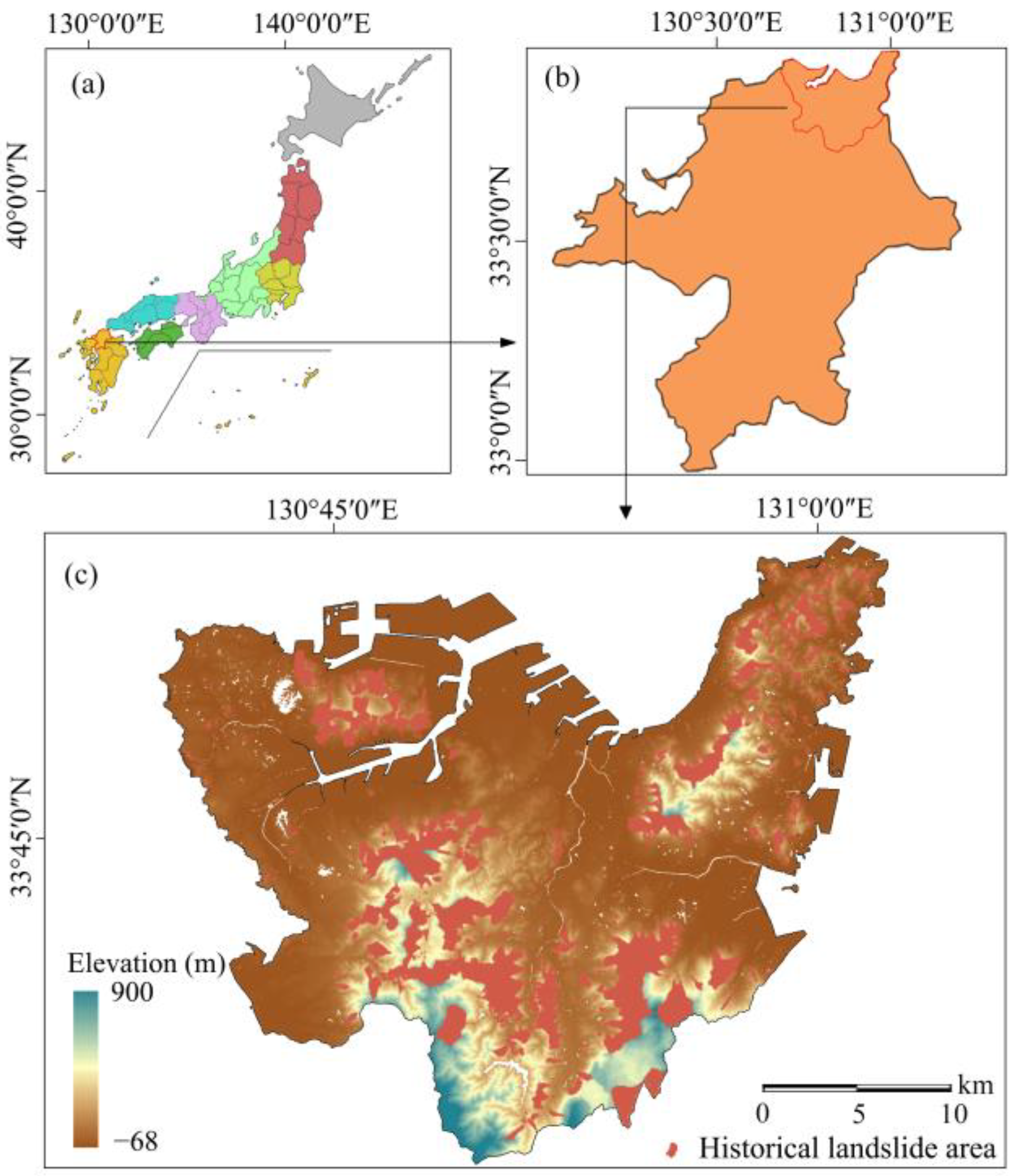
3.1. Study Area

In the present study, Kitakyushu, belonging to Fukuoka in Japan, was selected as the study area (Figure 3). Geographically, the area is located within 33°58′00″ N to 33°43′00″ N and 130°40′00″ E to 131°01′00″ E, with an area of 488.78 km2. Kitakyushu is on the northern Kyushu Island, and the southern side of the area is the hibikinada of the Japan Sea, while its eastern side is Suwou of SetoNaikai. Geologically, the whole area is characterized by rugged topography and tilting terrain from north to south. The highest and lowest altitudes of the study area are about 900 m and –68 m, respectively. Meanwhile, the area can be mainly divided into four regions: southern mountain region, central plain region, northeastern mountain region and northwestern hilly region. In accordance with the Ministry of Land, Infrastructure, Transport and Tourism of Japan, the study area has active geological tectonic movements with complex geological conditions. The lithology of the study area dominates sedimentary rock and igneous rocks, with a landfill area of more than 5% of the study area.
The annual average precipitation of the study area is about 1265 mm, which is the main inducing factor for landslides. The area is warm and humid throughout the year with an average annual temperature of 16.2 °C. Under the influence of the geographical environment, the northern region has a typical Japan Sea climate, while the eastern region has a Seto Inland Sea climate. The precipitation significantly varies, concentrated in the rainy season and typhoon season. Because the study area is located in the Pacific Rim Volcanic Seismic Zone at the junction of Eurasian and Pacific plates, it has frequent crustal movements. The heavy rainfall and crustal movement are thus factors inducing landslides.
Kitakyushu and Fukuoka are considered as the center of the metropolitan area and the hub of all administrative activities of the Kyushu area. According to the census of Japan, 2017, Kitakyushu has a population of 935,000. According to the Bureau of Land Policy in the Ministry of Land, Infrastructure, Transport and Tourism of Japan, the historical landslide areas can be obtained in Figure 3. The frequent landslides thus restrict the development of the industry and the socio-economic growth of the study area.

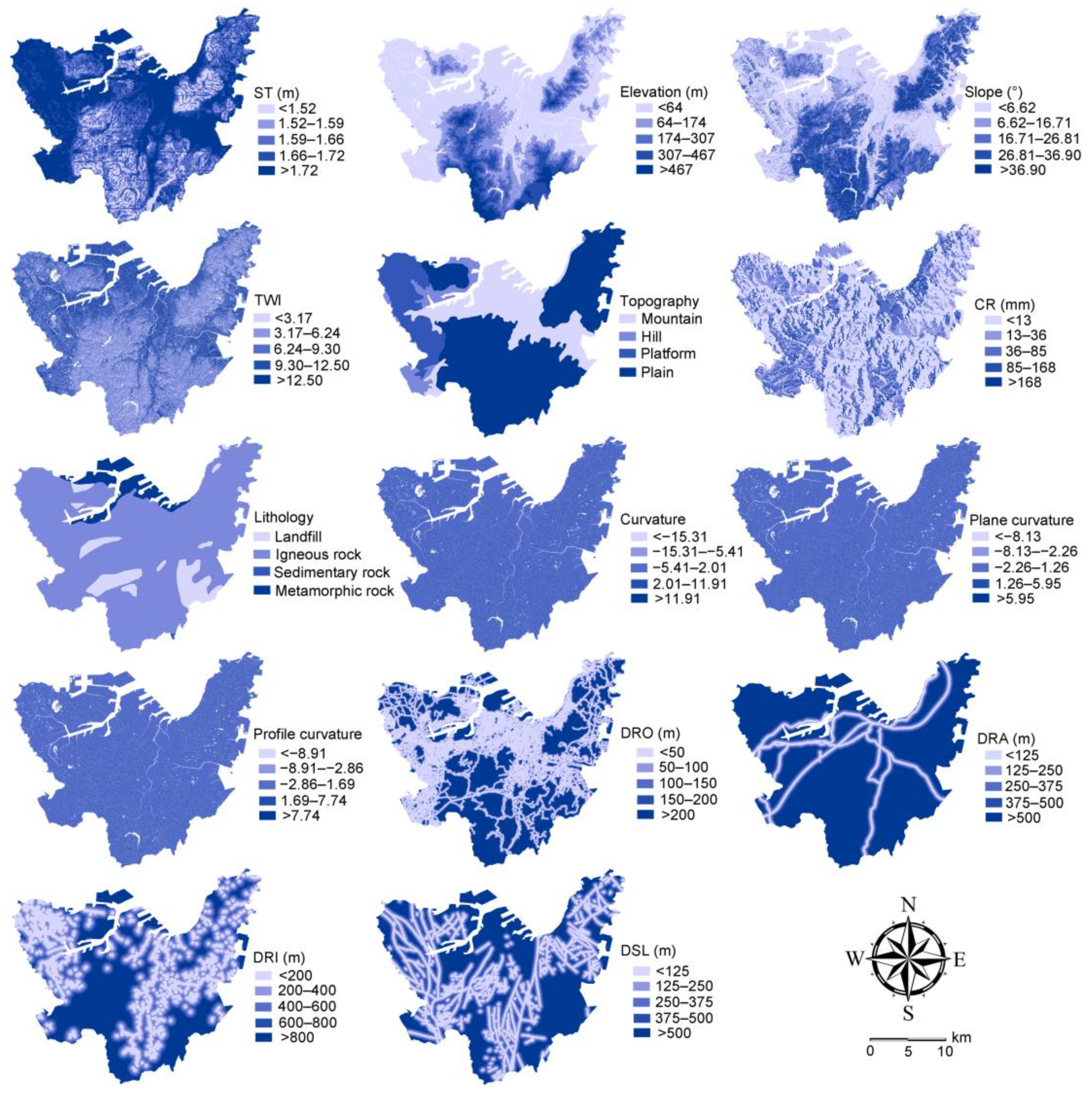
3.2. Condition Factors

Taking the appropriate relevant factors into consideration is essential for evaluating landslide susceptibility. Based on the previous survey study of the study area, the following 14 condition factors were collected and prepared: soil thickness (ST), elevation, slope, topographic wetness index (TWI), topography, cumulative runoff (CR), lithology, curvature, plane curvature, profile curvature, distance to the road (DRO), distance to the railway (DRA), distance to a river (DRI) and distance to a structure line (DSL).
The data of the condition factor were obtained by the field environmental survey and related literature research. The digital elevation model (DEM) data were provided by the Geospatial Information Authority of Japan, and the maps of elevation, slope, TWI, curvature, plane curvature and profile curvature in the study area were thus prepared. The geology factors, namely the soil thickness, topography, cumulative runoff, structure line and lithology, were provided by the Ministry of Land, Infrastructure, Transport and Tourism of Japan. Information about the roads, railways and rivers was provided by the Ministry of Land, Infrastructure, Transport and Tourism Kyushu Regional Development Bureau. The factors involve both quantitative and qualitative elements. The quantitative factors are divided into five levels using the natural breakpoint method, and Figure 4 shows the maps of the 14 factors.

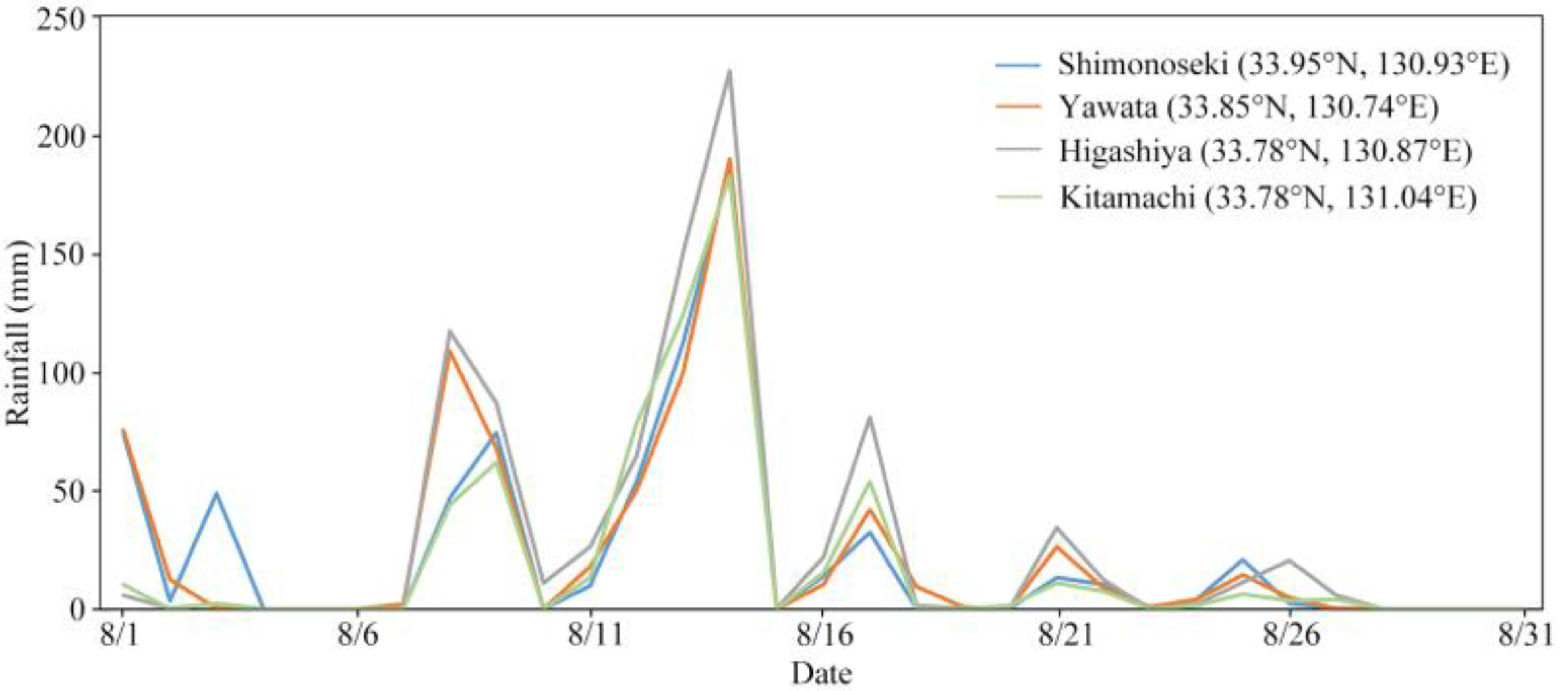
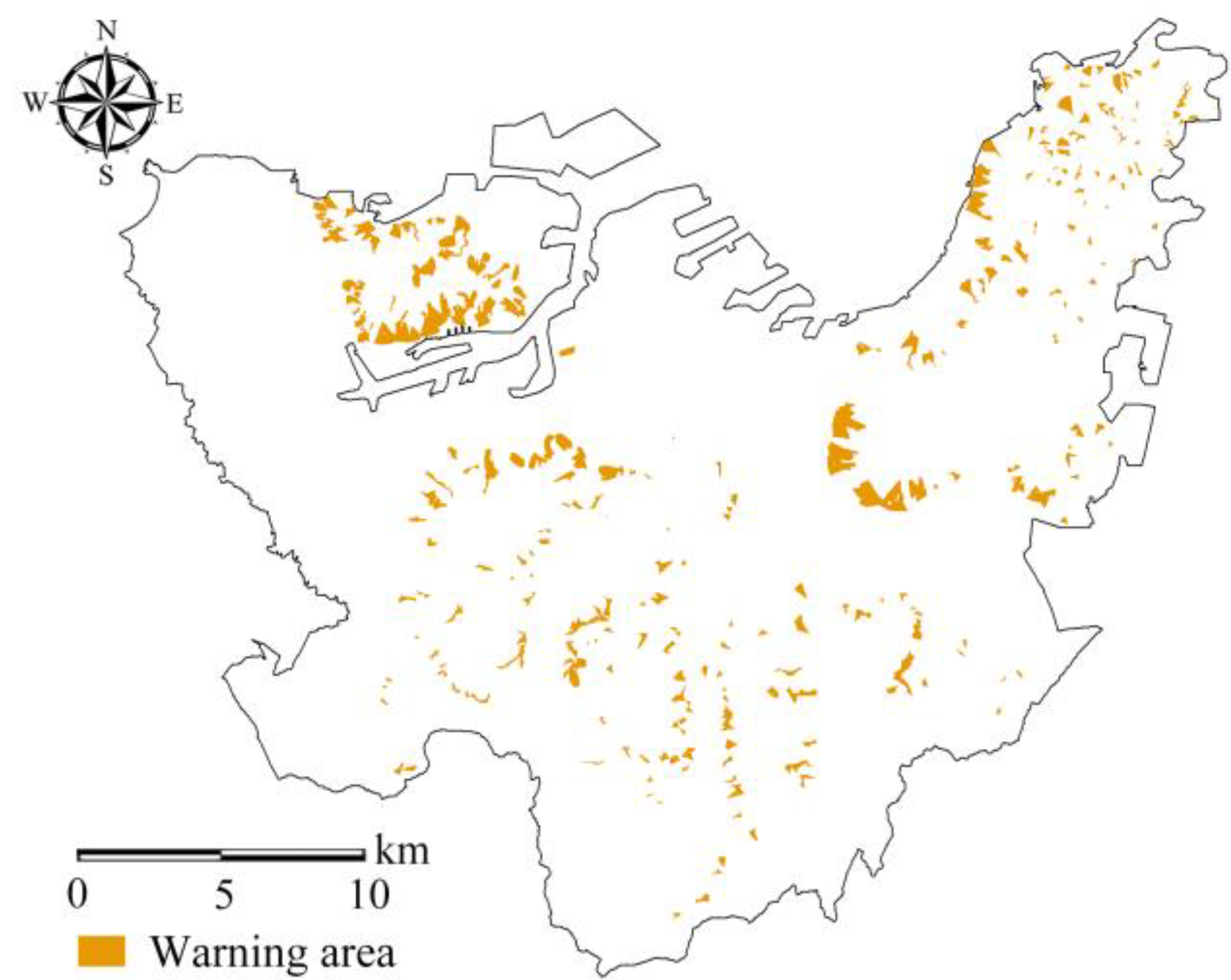
3.3. Heavy Rainfall Data and Landslide Warning Map

Heavy rainfall is one of the most significant landslide-inducing factors, and because of the climate characteristic of the rainy season in the study area, there always is heavy rainfall in August. The daily rainfalls in August at various monitoring stations are collected from the Japan Meteorological Agency of Ministry of Land, Infrastructure, Transport and Tourism (Figure 5).
As can be seen from Figure 5, the heavy rainfall started on 7 August and ended on 27 August. According to the rainfall variability and trends in Figure 5, the heavy rainfall can be divided into four stages, namely the development stage (from 7 August to 10 August), peak stage (from 11 August to 15 August), stagnation stage (from 16 August to 20 August) and decline stage (from 21 August to 27 August). Meanwhile, the geo-hazard warning map after the heavy rainfall also can be collected from the Japan Meteorological Agency of Ministry of Land, and the map is shown in Figure 6.

4. Results

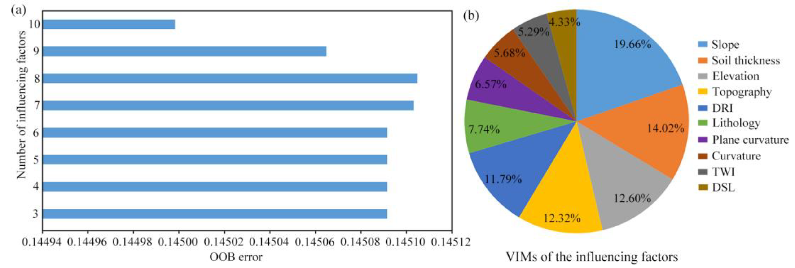
4.1. Selection of Spatial Influencing Factors

The spatial influencing factors are selected using the χ 2 test, OOB (out-of-bag) error and multicollinearity test. The χ 2 values of the 14 factors can be obtained using Statistical Product and Service Solutions (SPSS) in Table 1.
The χ 2 values of various factors are compared with the critical value (k = 3.84), and the factors whose χ 2 values are smaller than the critical value are eliminated. Therefore, 10 factors, namely the soil thickness, elevation, slope, TWI, topography, lithology, curvature, plane curvature, DRI and DSL, are selected as evaluation indices. According to the RFE, the OOB errors of various factor selection and the VIMs of selected factors are calculated, and the factor with the least VIM is eliminated. The process is repeated, and the OOB errors and VIMs are thus shown in Figure 7.
As can be seen from Figure 7a, the number of factors in the optimal factor selection is 10, and the VIMs of the 10 factors are shown in Figure 7b. The VIFs of the 10 factors are then obtained to verify the multicollinearity in Table 2.
As shown in Table 2, the VIFs are far less than 10, and this indicates there is no strong correlation between the factors, which proves that there is no redundancy in the factor selection.

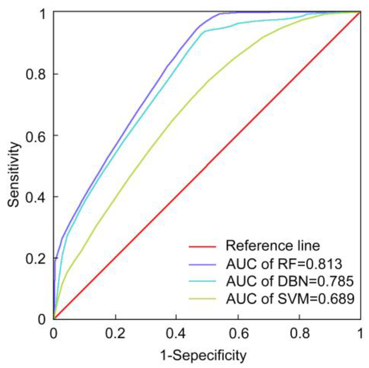
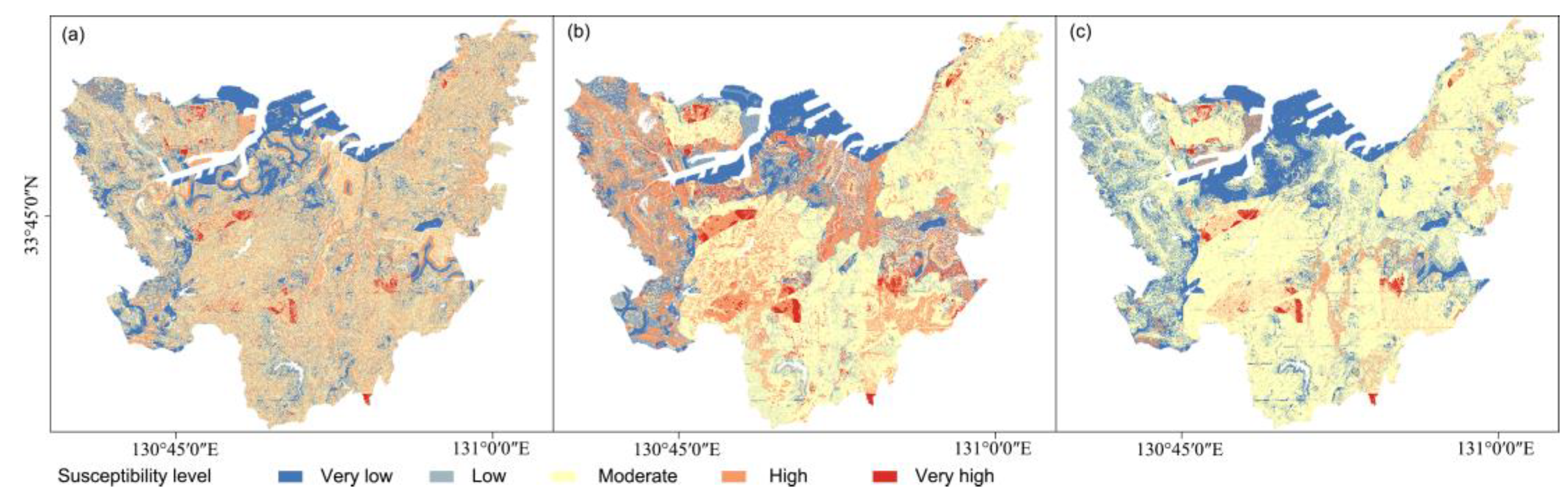
4.2. Spatial Landslide Susceptibility Mapping (LSMs) and Validation

The spatial landslide susceptibility of the study area is evaluated using the RF model, DBN model and SVM model. The landslide region is set to 1, while the non-landslide region is set to 0, and the map of historical landslide region is coupled with the maps of selected influencing factors. We selected 70% of grid data as the training data to predict the landslide susceptibility of each grid in the study area. The spatial LSMs were thus divided into five categories—very low susceptibility, low susceptibility, moderate susceptibility, high susceptibility and very high susceptibility—using a natural breakpoint method and shown in Figure 8, and the area percentages of various susceptibility levels are thus presented in Table 3.
As shown in the figure and table above, the distribution of the LSMs is similar, and the very low susceptibility area is mainly concentrated in the northern part of the study area. The area with the moderate susceptibility level is the largest area of the study area, while the area with the very high susceptibility level is the smallest. Then, the SCAI and ROC curve are used to verify the accuracy of the three LSMs using the RF model, DBN model and SVM model. The SCAI is an effective method to verify the accuracy of the three assessment results, and the SCAIs of various models are shown in Table 4.
Table 4 shows that the very high susceptibility has the smallest SCAI value, while the very low susceptibility has the greatest SCAI value. It indicates that the three models are applicable to the LSA in the study area. Meanwhile, the ROC curve and AUC are methods commonly used to evaluate quantitatively the accuracy of the assessment result, and they are thus drawn in Figure 9.
The ROC curves and AUCs illustrate that the RF model presents the best LSA performance. The RF model can be considered as the optimal model in the three models for the LSM in the study area.

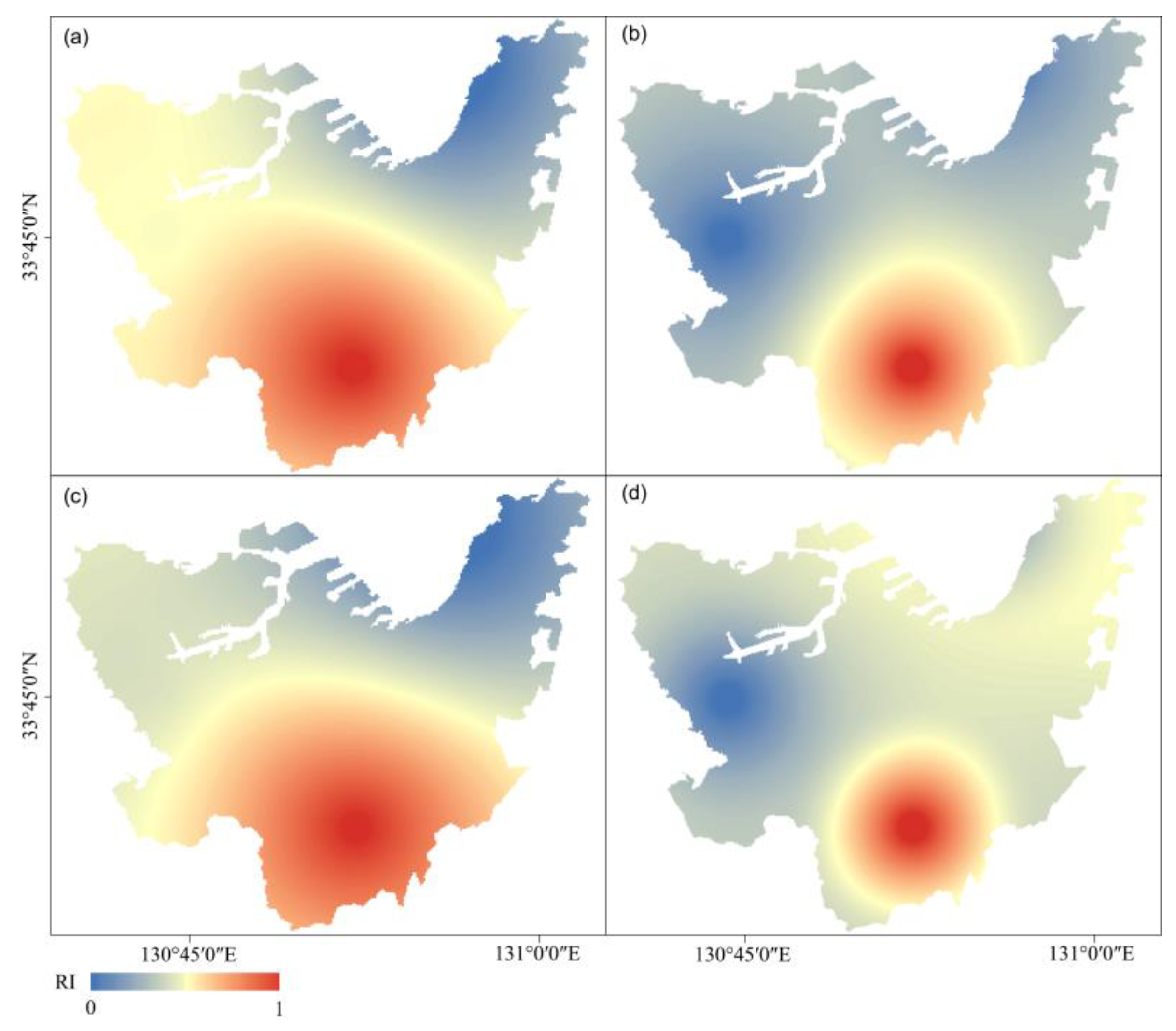
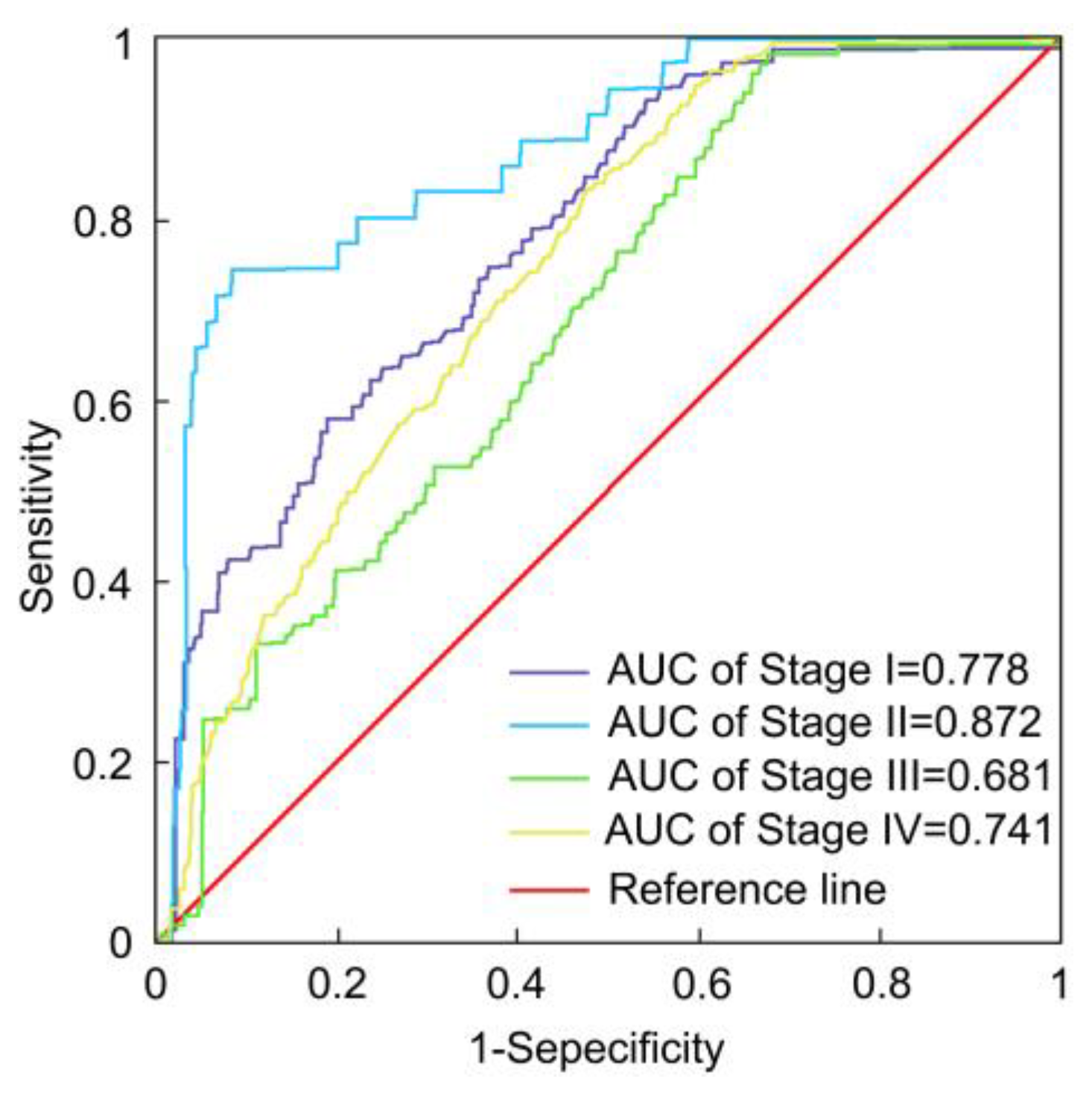
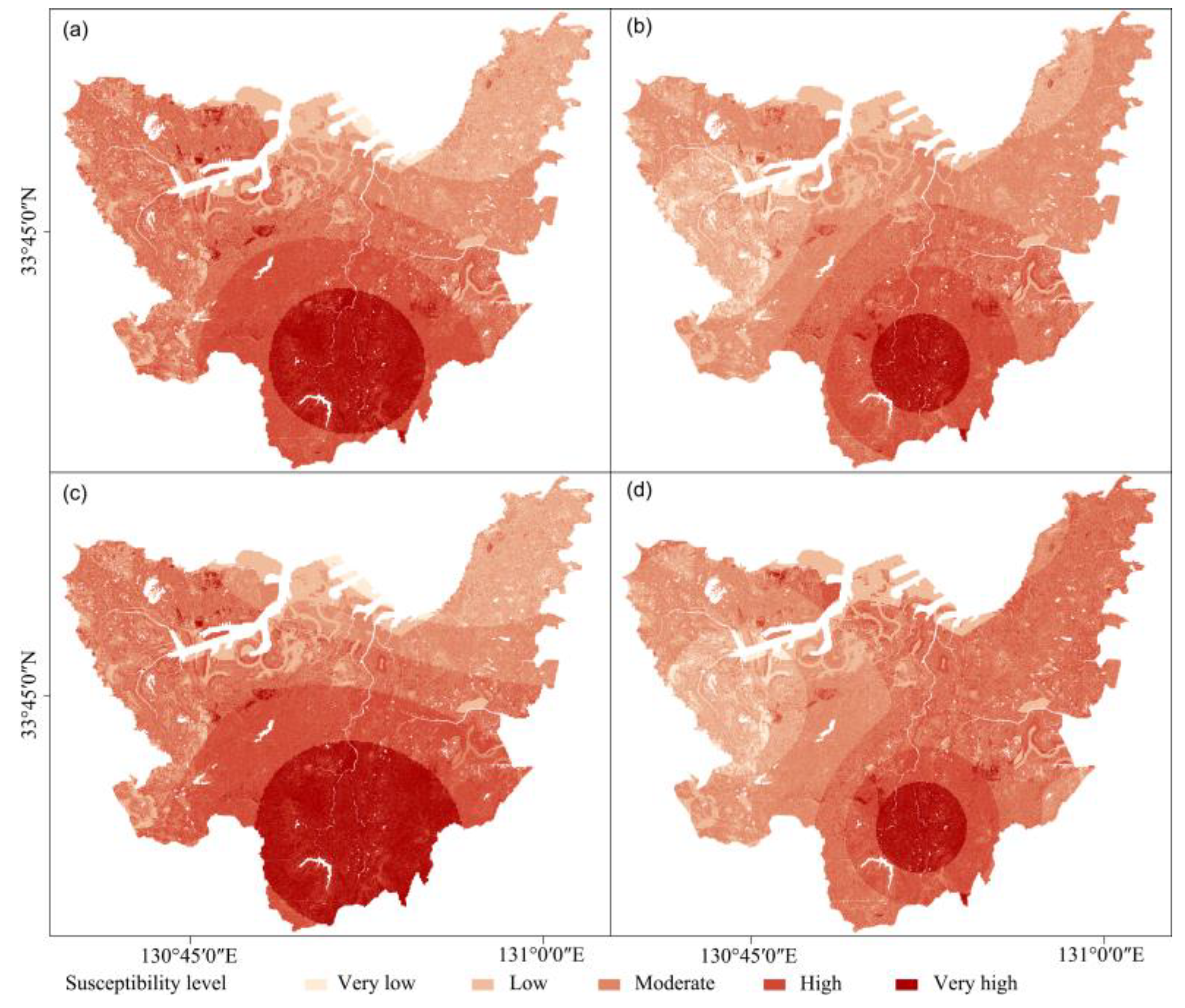
4.3. Spatiotemporal LSMs and Validation

There is always heavy rainfall in August in the study area, and the heavy rainfall is divided into four stages, namely the development stage, peak stage, stagnation stage and decline stage. The effective rainfall in the four stages is obtained using ERM to analyze the spatial impact of rainfall in the various stages on the landslide susceptibility. According to the rainfall data collected from various monitoring stations, the daily rainfall maps during the heavy rainfall period are thus obtained using kriging interpolation. The effective rainfall maps of the four stages are then generated, and the RI is normalized and calculated using Equation (13).
R I = E R E R m i n E R m a x E R m i n ,
where E R is the effective rainfall of the grid; E R m i n is the minimum effective rainfall in the study area; and E R m a x is the maximum effective rainfall in the study area. The RI maps are thus obtained and presented in Figure 10.
The RI maps of the four stages are coupled to the spatial assessment result using the optimal model. The temporal landslide probability, namely the RI, in the study area is thus accumulated with the spatial landslide probability obtained using the RF model to obtain the spatiotemporal LSA. The accumulation results are then divided into five categories: very low susceptibility, low susceptibility, moderate susceptibility, high susceptibility and very high susceptibility using the natural breakpoint method, and the spatiotemporal LSMs of the four stages are generated and shown in Figure 11.
Figure 11 shows that the spatiotemporal LSMs are tightly associated with the temporal LSAs, namely the RI maps. The area with the very high susceptibility is highly concentrated in the central-south region in the study area, while the area with the very low susceptibility is mainly located in the northern region. Meanwhile, the changes of the susceptibility assessment are fluctuating with the volatility of changing heavy rainfall. According to the geological hazard warning area after the heavy rainfall, the spatiotemporal LSMs are then validated using the ROC curve to determine the optimal stage used for spatiotemporal LSA. The ROC curves and AUC of the various stages are generated in Figure 12.
The above ROC curves indicate that the rainfall data in the development stage and peak stage show better applicability of the LSMs, and the spatiotemporal LSM result using the effective rainfall of the peak stage is the most accurate. The spatiotemporal LSM in the peak stage can be considered as the optimal spatiotemporal assessment result incorporating the effects of heavy rainfall.

5. Discussion

In previous studies, the spatial LSA has been investigated sufficiently, and the spatial LSMs are optimized from various aspects, such as the evaluation units, evaluation indices and evaluation models [6,51,52]. The spatial models perform well in evaluating spatial LSMs using the condition factors and historical landslides, but the temporal factors, such as climate change and heavy rainfall, may rapidly reshape the environment in the study area and thus increase the incidence of landslides. This further increases the landslide risk in the study area and reshapes the distribution of landslide susceptibility levels [53,54].
The present study considers the impact of condition factors and temporal factors based on the variability and trends of heavy rainfall in the study area. Although this study analyzes the fluctuating variation of the spatiotemporal LSA which is affected by volatility changes of heavy rainfall, the analysis may only be applied to the area where heavy rainfall is the main landslide-inducing factor. On the other hand, the spatial LSA in the previous study is validated using the historical landslide data, because they considered that the areas under the same spatial conditions as the landslide area are more prone to landslides. However, real-time rainfall data need to be employed to analyze the temporal LSA, and it is thus inaccurate to validate the accuracy of spatiotemporal LSA using historical landslide data. The future landslide data or landslide warning area can be used for the spatiotemporal LSA validation, however, it is difficult to implement if there is no landslide warning map because it is hard to collect the future landslide data.

6. Conclusions

In heavy rainfall areas, rainfall-induced landslides are always an important threat. The present study thus proposes a methodology to generate a spatiotemporal LSM, and the proposed method is applied to Kitakyushu, Fukuoka, Japan, under the impact of heavy rainfall in August 2021. The condition factors are selected as evaluation indices using the χ 2 test, OOB error and multicollinearity test. The spatial LSMs are then generated using the RF model, DBN model and SVM model, and the results are compared and verified using ROC curves, AUCs and SCAIs to determine that the RF model is the optimal model for the spatial LSM in the study area. According to the rainfall variability and trends, the heavy rainfall period is divided into four stages, and the RI maps of various stages are obtained using ERM. The spatiotemporal LSMs under the influence of heavy rainfall in August are generated by coupling the four RI maps with the landslide probability map obtained using the RF model, and the changes of the susceptibility assessment are fluctuating over time. The spatiotemporal LSMs of various stages are verified using the landslide warning map, which illustrates that the four spatiotemporal results are accurate and the evaluation performance of spatiotemporal LSMs with the spatial LSM obtained using the RF model and RI map of the peak stage is the highest. The proposed method is scientific and feasible in spatiotemporal LSA and useful for areas with rainfall-induced landslides threatening human lives and property.

Author Contributions

J.L. lead the research program; J.L. and W.W. wrote the manuscript. Y.L., Z.H. and G.C. reviewed and edited the manuscript. All authors have read and agreed to the published version of the manuscript.

Funding

This research was funded by the High-Speed Railway Infrastructure Joint Fund of the National Natural Science Foundation of China (No. U1734208) and the National Natural Science Foundation of China (Grant No. 51478483, W. Wang). The financial supports are gratefully acknowledged.

Institutional Review Board Statement

Not applicable.

Informed Consent Statement

Not applicable.

Data Availability Statement

The data used in this study are available on request from the corresponding author.

Conflicts of Interest

The authors declare no conflict of interest.

References

  1. Wang, W.; Li, J.; Qu, X.; Han, Z.; Liu, P. Prediction on landslide displacement using a new combination model: A case study of Qinglong landslide in China. Nat. Hazard. 2019, 96, 1121–1139. [Google Scholar] [CrossRef]
  2. Li, J.; Wang, W.; Han, Z. A variable weight combination model for prediction on landslide displacement using AR model, LSTM model, and SVM model: A case study of the Xinming landslide in China. Environ. Earth Sci. 2021, 80, 386. [Google Scholar] [CrossRef]
  3. Wang, W.-D.; Li, J.; Han, Z. Comprehensive assessment of geological hazard safety along railway engineering using a novel method: A case study of the Sichuan-Tibet railway, China. Geomat. Nat. Hazards Risk 2020, 11, 1–21. [Google Scholar] [CrossRef] [Green Version]
  4. Li, J.; Wang, W.-D.; Han, Z.; Chen, G. Analysis of secondary-factor combinations of landslides using improved association rule algorithms: A case study of Kitakyushu in Japan. Geomat. Nat. Hazards Risk 2021, 12, 1885–1904. [Google Scholar] [CrossRef]
  5. Zhang, S.; Xu, D.; Shen, G.; Liu, J.; Yang, L. Numerical Simulation of Na-Tech Cascading Disasters in a Large Oil Depot. Int. J. Environ. Res. Public Health 2020, 17, 8620. [Google Scholar] [CrossRef] [PubMed]
  6. Li, J.; Wang, W.-D.; Han, Z.; Li, Y.; Chen, G. Exploring the Impact of Multitemporal DEM Data on the Susceptibility Mapping of Landslides. Appl. Sci. 2020, 10, 2518. [Google Scholar] [CrossRef] [Green Version]
  7. Xing, X.; Wu, C.; Li, J.; Li, X.; He, R. Susceptibility assessment for rainfall-induced landslides using a revised logistic regression method. Nat. Hazard. 2021, 106, 97–117. [Google Scholar] [CrossRef]
  8. Liu, X.; Wang, Y. Probabilistic simulation of entire process of rainfall-induced landslides using random finite element and material point methods with hydro-mechanical coupling. Comput. Geotech. 2021, 132, 103989. [Google Scholar] [CrossRef]
  9. Calcaterra, D.; Parise, M.; Palma, B.; Pelella, L. The influence of meteoric events in triggering shallow landslides in pyroclastic deposits of Campania, Italy. In Landslides in Research, Theory and Practice, Proceedings of the 8th International Symposium on Landslides, Cardiff, UK, 26–30 June 2000; Thomas Telford Publishing: London, UK, 2000. [Google Scholar]
  10. Andrea, C.; Pierluigi, B.; Claudia, S.; Ivano, R. Relationships between geo-hydrological processes induced by heavy rainfall and land-use: The case of 25 October 2011 in the Vernazza catchment (Cinque Terre, NW Italy). J. Maps 2013, 9, 289–298. [Google Scholar] [CrossRef]
  11. Bordoni, M.; Meisina, C.; Valentino, R.; Lu, N.; Bittelli, M.; Chersich, S. Hydrological factors affecting rainfall-induced shallow landslides: From the field monitoring to a simplified slope stability analysis. Eng. Geol. 2015, 193, 19–37. [Google Scholar] [CrossRef]
  12. Ng, C.; Yang, B.; Liu, Z.Q.; Kwan, J.; Chen, L. Spatiotemporal modelling of rainfall-induced landslides using machine learning. Landslides 2021, 18, 2499–2514. [Google Scholar] [CrossRef]
  13. Dahal, R.K.; Hasegawa, S.; Nonomura, A.; Yamanaka, M.; Masuda, T.; Nishino, K. GIS-based weights-of-evidence modelling of rainfall-induced landslides in small catchments for landslide susceptibility mapping. Environ. Geol. 2008, 54, 311–324. [Google Scholar] [CrossRef]
  14. Schilirò, L.; Cepeda, J.; Devoli, G.; Piciullo, L. Regional Analyses of Rainfall-Induced Landslide Initiation in Upper Gudbrandsdalen (South-Eastern Norway) Using TRIGRS Model. Geosciences 2021, 11, 35. [Google Scholar] [CrossRef]
  15. Roessner, S.; Wetzel, H.U.; Kaufmann, H.; Sarnagoev, A. Potential of Satellite Remote Sensing and GIS for Landslide Hazard Assessment in Southern Kyrgyzstan (Central Asia). Nat. Hazard. 2005, 35, 395–416. [Google Scholar] [CrossRef]
  16. Wu, C. Landslide Susceptibility Based on Extreme Rainfall-Induced Landslide Inventories and the Following Landslide Evolution. Water 2019, 11, 2609. [Google Scholar] [CrossRef] [Green Version]
  17. Choi, J.; Oh, H.J.; Lee, H.J.; Lee, C.; Lee, S. Combining landslide susceptibility maps obtained from frequency ratio, logistic regression, and artificial neural network models using ASTER images and GIS. Eng. Geol. 2012, 124, 12–23. [Google Scholar] [CrossRef]
  18. Pourghasemi, H.R.; Sadhasivam, N.; Amiri, M.; Eskandari, S.; Santosh, M. Landslide susceptibility assessment and mapping using state-of-the art machine learning techniques. Nat. Hazard. 2021, 108, 1291–1316. [Google Scholar] [CrossRef]
  19. Goyes-Peñafiel, P.; Hernandez-Rojas, A. Landslide susceptibility index based on the integration of logistic regression and weights of evidence: A case study in Popayan, Colombia. Eng. Geol. 2021, 280, 105958. [Google Scholar] [CrossRef]
  20. Mandal, K.; Saha, S.; Mandal, S. Applying deep learning and benchmark machine learning algorithms for landslide susceptibility modelling in Rorachu river basin of Sikkim Himalaya, India. Geosci. Front. 2021, 12, 101203. [Google Scholar] [CrossRef]
  21. Tanyu, B.F.; Abbaspour, A.; Alimohammadlou, Y.; Tecuci, G. Landslide susceptibility analyses using Random Forest, C4.5, and C5.0 with balanced and unbalanced datasets. CATENA 2021, 203, 105355. [Google Scholar] [CrossRef]
  22. Hong, H.; Tsangaratos, P.; Ilia, I.; Loupasakis, C.; Wang, Y. Introducing a novel multi-layer perceptron network based on stochastic gradient descent optimized by a meta-heuristic algorithm for landslide susceptibility mapping. Sci. Total Environ. 2020, 742, 140549. [Google Scholar] [CrossRef] [PubMed]
  23. García-Rodríguez, M.; Malpica, J.A. Assessment of earthquake-triggered landslide susceptibility in El Salvador based on an Artificial Neural Network model. Nat. Hazards Earth Syst. Sci. 2010, 10, 1307–1315. [Google Scholar] [CrossRef]
  24. Chen, X.; Chen, W. GIS-based landslide susceptibility assessment using optimized hybrid machine learning methods. CATENA 2021, 196, 104833. [Google Scholar] [CrossRef]
  25. Hong, H.; Aiding, K.; Adel, S.; Razavi, T.; Liu, J.; Zhu, A.X.; Yari, H.A.; Bin, A.B.; Wang, Y. Landslide susceptibility assessment in the Anfu County, China: Comparing different statistical and probabilistic models considering the new topo-hydrological factor (HAND). Earth Sci. Inform. 2018, 11, 605–622. [Google Scholar] [CrossRef]
  26. Du, J.; Glade, T.; Woldai, T.; Chai, B.; Zeng, B. Landslide susceptibility assessment based on an incomplete landslide inventory in the Jilong Valley, Tibet, Chinese Himalayas. Eng. Geol. 2020, 270, 105572. [Google Scholar] [CrossRef]
  27. Nepal, N.; Chen, J.; Chen, H.; Wang, X.A.; Pangali Sharma, T.P. Assessment of landslide susceptibility along the Araniko Highway in Poiqu/Bhote Koshi/Sun Koshi Watershed, Nepal Himalaya. Prog. Disaster Sci. 2019, 3, 100037. [Google Scholar] [CrossRef]
  28. Saha, A.; Saha, S. Comparing the efficiency of weight of evidence, support vector machine and their ensemble approaches in landslide susceptibility modelling: A study on Kurseong region of Darjeeling Himalaya, India. Remote Sens. Appl. Soc. Environ. 2020, 19, 100323. [Google Scholar] [CrossRef]
  29. Ozdemir, A.; Altural, T. A comparative study of frequency ratio, weights of evidence and logistic regression methods for landslide susceptibility mapping: Sultan Mountains, SW Turkey. J. Asian Earth Sci. 2013, 64, 180–197. [Google Scholar] [CrossRef]
  30. Wang, Y.; Feng, L.; Li, S.; Ren, F.; Du, Q. A hybrid model considering spatial heterogeneity for landslide susceptibility mapping in Zhejiang Province, China. CATENA 2020, 188, 104425. [Google Scholar] [CrossRef]
  31. Hu, Q.; Zhou, Y.; Wang, S.; Wang, F. Machine learning and fractal theory models for landslide susceptibility mapping: Case study from the Jinsha River Basin. Geomorphology 2020, 351, 106975. [Google Scholar] [CrossRef]
  32. Thi Ngo, P.T.; Panahi, M.; Khosravi, K.; Ghorbanzadeh, O.; Kariminejad, N.; Cerda, A.; Lee, S. Evaluation of deep learning algorithms for national scale landslide susceptibility mapping of Iran. Geosci. Front. 2021, 12, 505–519. [Google Scholar] [CrossRef]
  33. Wang, Y.; Fang, Z.; Wang, M.; Peng, L.; Hong, H. Comparative study of landslide susceptibility mapping with different recurrent neural networks. Comput. Geosci. 2020, 138, 104445. [Google Scholar] [CrossRef]
  34. Hoang, N.D.; Tien Bui, D. Spatial prediction of rainfall-induced shallow landslides using gene expression programming integrated with GIS: A case study in Vietnam. Nat. Hazard. 2018, 92, 1871–1887. [Google Scholar] [CrossRef]
  35. Tseng, C.-M.; Chen, Y.-R.; Wu, S.-M. Scale and spatial distribution assessment of rainfall-induced landslides in a catchment with mountain roads. Nat. Hazards Earth Syst. Sci. 2018, 18, 687–708. [Google Scholar] [CrossRef] [Green Version]
  36. Conte, E.; Troncone, A. Stability analysis of infinite clayey slopes subjected to pore pressure changes. Géotechnique 2012, 62, 87–91. [Google Scholar] [CrossRef]
  37. Conte, E.; Troncone, A. Analytical Method for Predicting the Mobility of Slow-Moving Landslides owing to Groundwater Fluctuations. J. Geotech. Geoenviron. Eng. 2011, 137, 777–784. [Google Scholar] [CrossRef]
  38. Baymani-Nezhad, M.; Han, D. Hydrological modeling using Effective Rainfall routed by the Muskingum method (ERM). J. Hydroinf. 2013, 15, 1437–1455. [Google Scholar] [CrossRef]
  39. Ma, T.; Li, C.; Lu, Z.; Wang, B. An effective antecedent precipitation model derived from the power-law relationship between landslide occurrence and rainfall level. Geomorphology 2014, 216, 187–192. [Google Scholar] [CrossRef]
  40. Akinwande, O.; Dikko, H.G.; Agboola, S. Variance Inflation Factor: As a Condition for the Inclusion of Suppressor Variable(s) in Regression Analysis. Open J. Stat. 2015, 05, 754–767. [Google Scholar] [CrossRef] [Green Version]
  41. Garcia, C.; Pérez, J.; López Martín, M.; Salmerón, R. Collinearity: Revisiting the variance inflation factor in ridge regression. J. Appl. Stat. 2015, 42, 648–661. [Google Scholar] [CrossRef]
  42. Sun, D.; Wen, H.; Wang, D.; Xu, J. A random forest model of landslide susceptibility mapping based on hyperparameter optimization using Bayes algorithm. Geomorphology 2020, 362, 107201. [Google Scholar] [CrossRef]
  43. Wang, W.; He, Z.; Han, Z.; Li, Y.; Dou, J.; Huang, J. Mapping the susceptibility to landslides based on the deep belief network: A case study in Sichuan Province, China. Nat. Hazards 2020, 103, 3239–3261. [Google Scholar] [CrossRef]
  44. Youssef, A.M.; Pourghasemi, H.R.; Pourtaghi, Z.S.; Al-Katheeri, M.M. Landslide susceptibility mapping using random forest, boosted regression tree, classification and regression tree, and general linear models and comparison of their performance at Wadi Tayyah Basin, Asir Region, Saudi Arabia. Landslides 2016, 13, 839–856. [Google Scholar] [CrossRef]
  45. Sun, D.; Xu, J.; Wen, H.; Wang, Y. An Optimized Random Forest Model and Its Generalization Ability in Landslide Susceptibility Mapping: Application in Two Areas of Three Gorges Reservoir, China. J. Earth Sci. 2020, 31, 1068–1086. [Google Scholar] [CrossRef]
  46. Xie, X.A.; Fu, G.A.; Xue, Y.A.; Zhao, Z.A.; Chen, P.A.; Lu, B.B.; Jiang, S.C. Risk prediction and factors risk analysis based on IFOA-GRNN and apriori algorithms: Application of artificial intelligence in accident prevention. Process Saf. Environ. Prot. 2019, 122, 169–184. [Google Scholar] [CrossRef]
  47. Lü, Q.; Dou, Y.; Niu, X.; Xu, J.; Xia, F. Remote Sensing Image Classification Based on DBN Model. J. Comput. Res. Dev. 2014, 51, 1911–1918. [Google Scholar]
  48. Kohler, M.; Richards, M. Multicapacity Basin Accounting for Predicting Runoff from Storm Precipitation. J. Geophys. Res. 1962, 67, 5187–5197. [Google Scholar] [CrossRef]
  49. Alatorre, L.C.; Raquel, S.A.; Santos, C.; Santiago, B.; Salvador, S.C. Identification of Mangrove Areas by Remote Sensing: The ROC Curve Technique Applied to the Northwestern Mexico Coastal Zone Using Landsat Imagery. Remote Sens. 2011, 3, 1568–1583. [Google Scholar] [CrossRef] [Green Version]
  50. Tsangaratos, P.; Ilia, I.; Hong, H.; Chen, W.; Xu, C. Applying Information Theory and GIS-based quantitative methods to produce landslide susceptibility maps in Nancheng County, China. Landslides 2017, 14, 1091–1111. [Google Scholar] [CrossRef]
  51. Napoli, M.; Carotenuto, F.; Cevasco, A.; Confuorto, P.; Calcaterra, D. Machine learning ensemble modelling as a tool to improve landslide susceptibility mapping reliability. Landslides 2020, 17, 1897–1914. [Google Scholar] [CrossRef]
  52. Li, Y.; Liu, X.; Han, Z.; Dou, J. Spatial Proximity-Based Geographically Weighted Regression Model for Landslide Susceptibility Assessment: A Case Study of Qingchuan Area, China. Appl. Sci. 2020, 10, 1107. [Google Scholar] [CrossRef] [Green Version]
  53. Mukherji, A.; Scott, C.; Molden, D.; Maharjan, A. Megatrends in Hindu Kush Himalaya: Climate Change, Urbanisation and Migration and Their Implications for Water, Energy and Food. In Assessing Global Water Megatrends; Springer: Singapore, 2018. [Google Scholar]
  54. Wester, P.; Mishra, A.; Mukherji, A.; Shrestha, A.B. The Hindu Kush Himalaya Assessment: Mountains, Climate Change, Sustainability and People; Springer Nature: Cham, Switzerland, 2019. [Google Scholar]
Figure 1. Schematic flowchart representing the methodology.
Water 13 03312 g001
Figure 2. Structure of deep belief networks (DBN) model.
Water 13 03312 g002
Figure 3. Location map of the study area showing: (a) Japan; (b) Fukuoka; and (c) Kitakyushu.
Water 13 03312 g003
Figure 4. Maps of landslide influencing factors, namely soil thickness, elevation, slope, topographic wetness index (TWI), topography, cumulative runoff, lithology, curvature, plane curvature, profile curvature, distance to the road (DRO), distance to the railway (DRA), distance to a river (DRI) and distance to a structure line (DSL).
Water 13 03312 g004
Figure 5. Daily rainfalls in August at various monitoring stations.
Water 13 03312 g005
Figure 6. Warning area map of the study area after heavy rainfall.
Water 13 03312 g006
Figure 7. (a) Out-of-bag (OOB) errors of various factor selections and (b) variable importance measures (VIMs) of selected factors.
Water 13 03312 g007
Figure 8. Landslide susceptibility mappings (LSMs) obtained using (a) random forest (RF) model; (b) deep belief network (DBN) model; and (c) support vector machine (SVM) model.
Water 13 03312 g008
Figure 9. Receiver operating characteristic (ROC) curves and areas under the curve (AUCs) of the three models.
Water 13 03312 g009
Figure 10. Rainfall impact (RI) maps of (a) development stage; (b) peak stage; (c) stagnation stage; and (d) decline stage.
Water 13 03312 g010
Figure 11. Spatiotemporal LSMs of (a) development stage; (b) peak stage; (c) stagnation stage; and (d) decline stage.
Water 13 03312 g011
Figure 12. ROC curves and AUCs of the four stages.
Water 13 03312 g012
Table 1. χ 2 values of the 14 factors.
Factors χ 2   Values Factors χ 2   Values
Soil thickness36.77Curvature 5.85
Elevation41.27Plane curvature8.15
Slope31.71Profile curvature3.10
TWI9.56DRO3.10
Topography 27.77DRA3.22
Cumulative runoff0.73DRI10.79
Lithology 14.73DSL4.60
Table 2. Variance inflation factors (VIFs) of the 10 factors.
FactorsVIFsFactorsVIFs
Slope1.327Lithology1.105
Soil thickness1.186Plane curvature1.109
Elevation1.446Curvature1.103
Topography1.384TWI1.173
DRI1.078DSL1.033
Table 3. Area percentages of various susceptibility levels.
ModelsVery LowLowModerateHighVery High
RF model15.25%15.30%40.05%27.45%1.95%
DBN model12.27%9.48%53.62%19.13%5.50%
SVM model20.14%1.16%71.37%6.24%1.09%
Table 4. Seed cell area indexes (SCAIs) of RF model, DBN model and SVM model.
ModelLevelArea PercentageLandslide Area (km2)Landslide PercentageSCAI
RF modelVery low15.25%0.2080.24%63.40
Low15.30%12.88814.90%1.03
Moderate40.05%40.60346.95%0.85
High27.45%26.34230.46%0.90
Very high1.95%6.4437.45%0.26
DBN modelVery low12.27%0.3670.42%28.91
Low9.48%0.4820.56%17.01
Moderate53.62%57.36866.34%0.81
High19.13%18.39121.27%0.90
Very high5.50%9.87611.42%0.48
SVM modelVery low20.14%1.6681.93%10.44
Low1.16%2.3962.77%0.42
Moderate71.37%73.13584.57%0.84
High6.24%4.9555.73%1.09
Very high1.09%4.3295.01%0.22
Publisher’s Note: MDPI stays neutral with regard to jurisdictional claims in published maps and institutional affiliations.

