
Dynamic Assessment of the Flood Risk at Basin Scale under Simulation of Land-Use Scenarios and Spatialization Technology of Factor


 , and
, and
Abstract
:1. Introduction
2. Materials
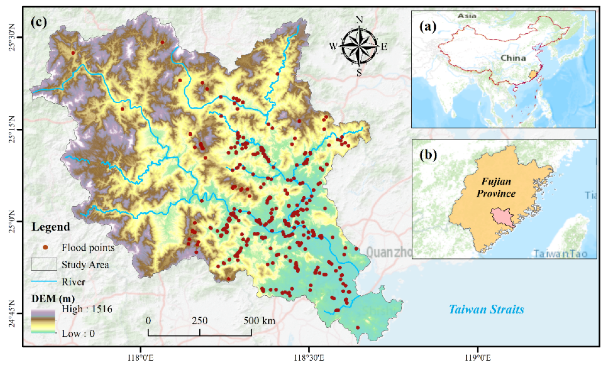
2.1. Study Area
2.2. Data
3. Methods
3.1. Land-Use Simulation Models
3.1.1. Markov Chain Model
3.1.2. The FLUS Model and Accuracy Verification
3.2. Land-Use Simulation Scenario Setting
3.3. Spatialization of Epigenetic Factors in Land Use
3.4. Flood Risk Determination Methods
3.4.1. Triangular Fuzzy Number-Based AHP (TFN-AHP)
3.4.2. Criteria Importance through Intercriteria Correlation (CRITIC)
3.4.3. Technique for Order Preference by Similarity to an Ideal Solution (TOPSIS)
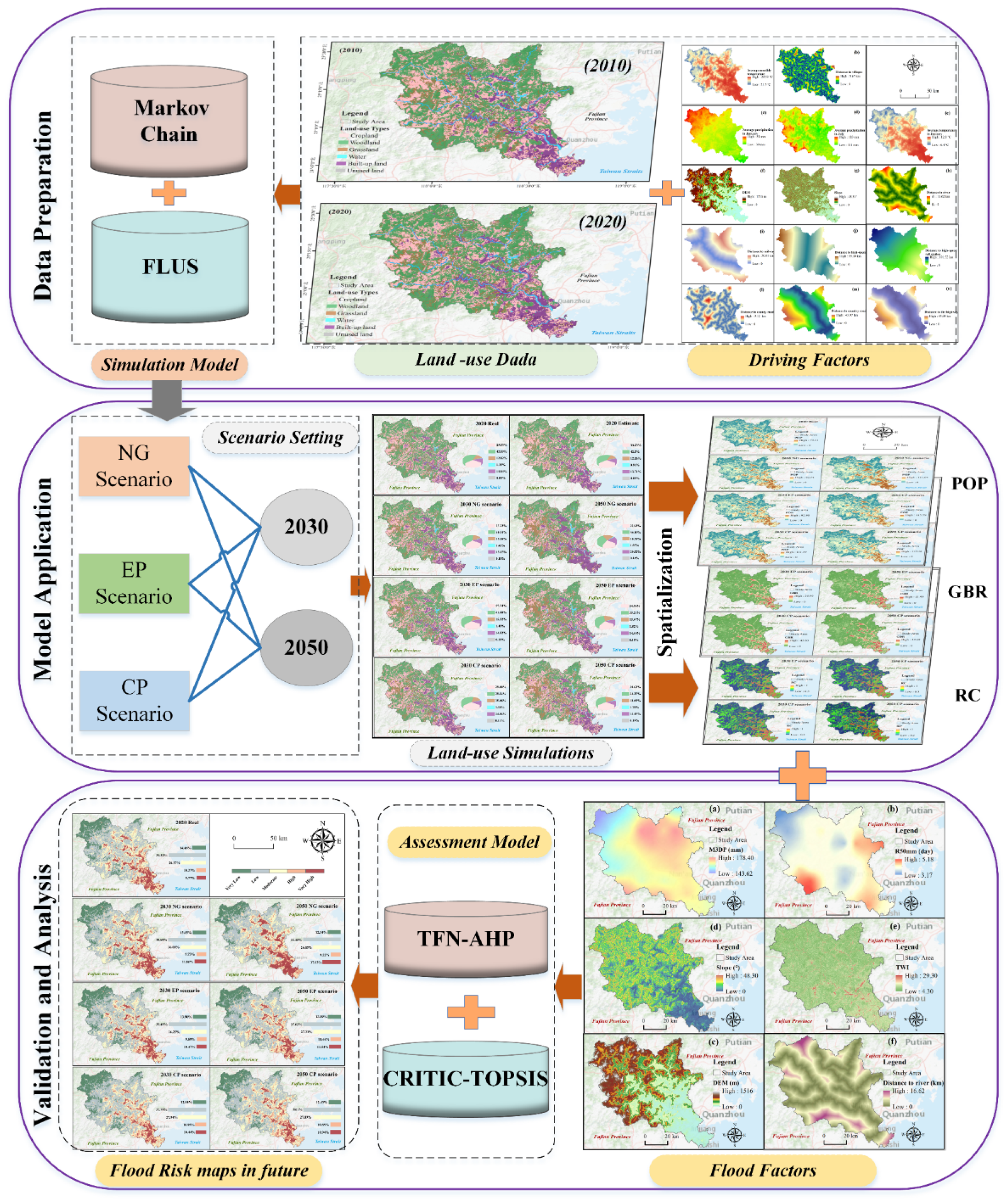
3.5. Processing
4. Results
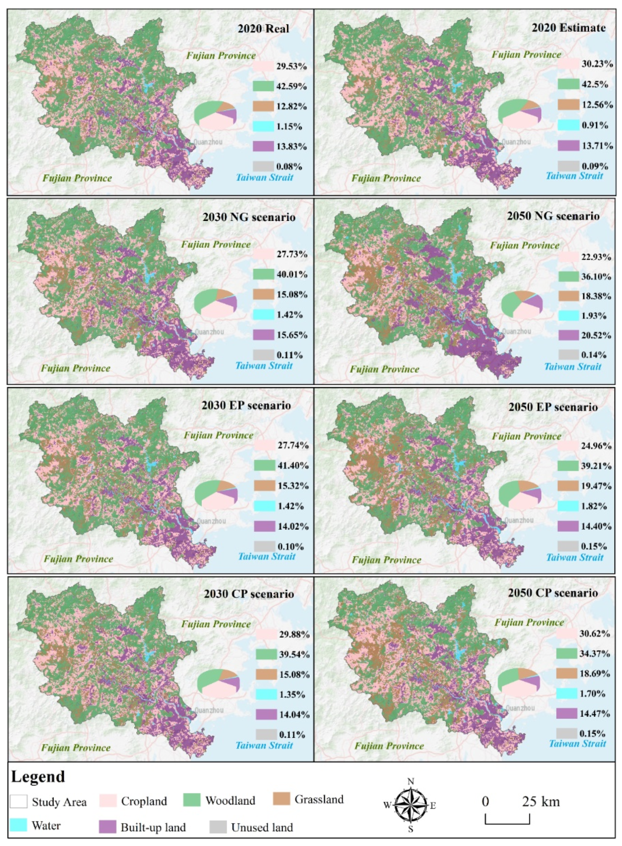
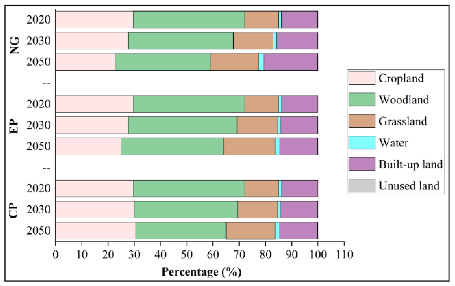
4.1. Land-Use Type Changes Based on Different Scenarios
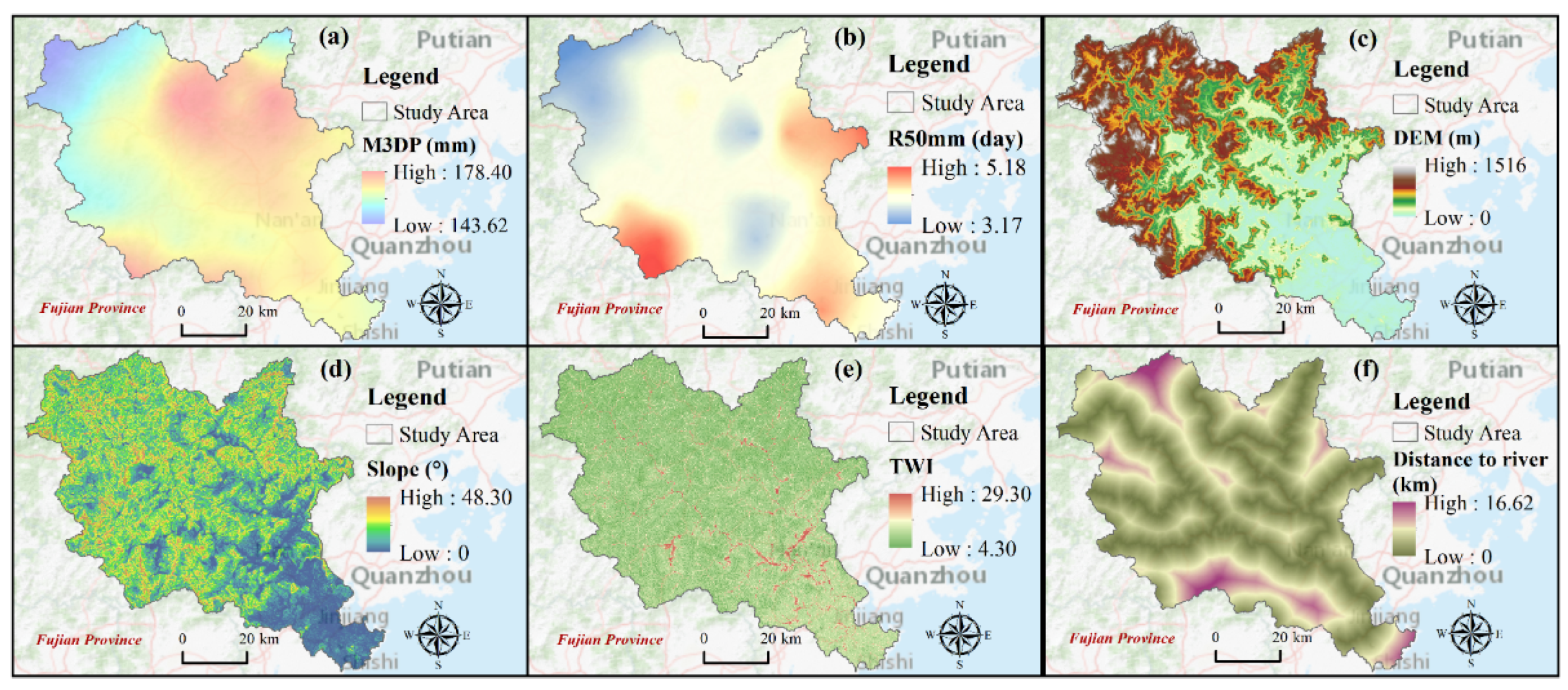
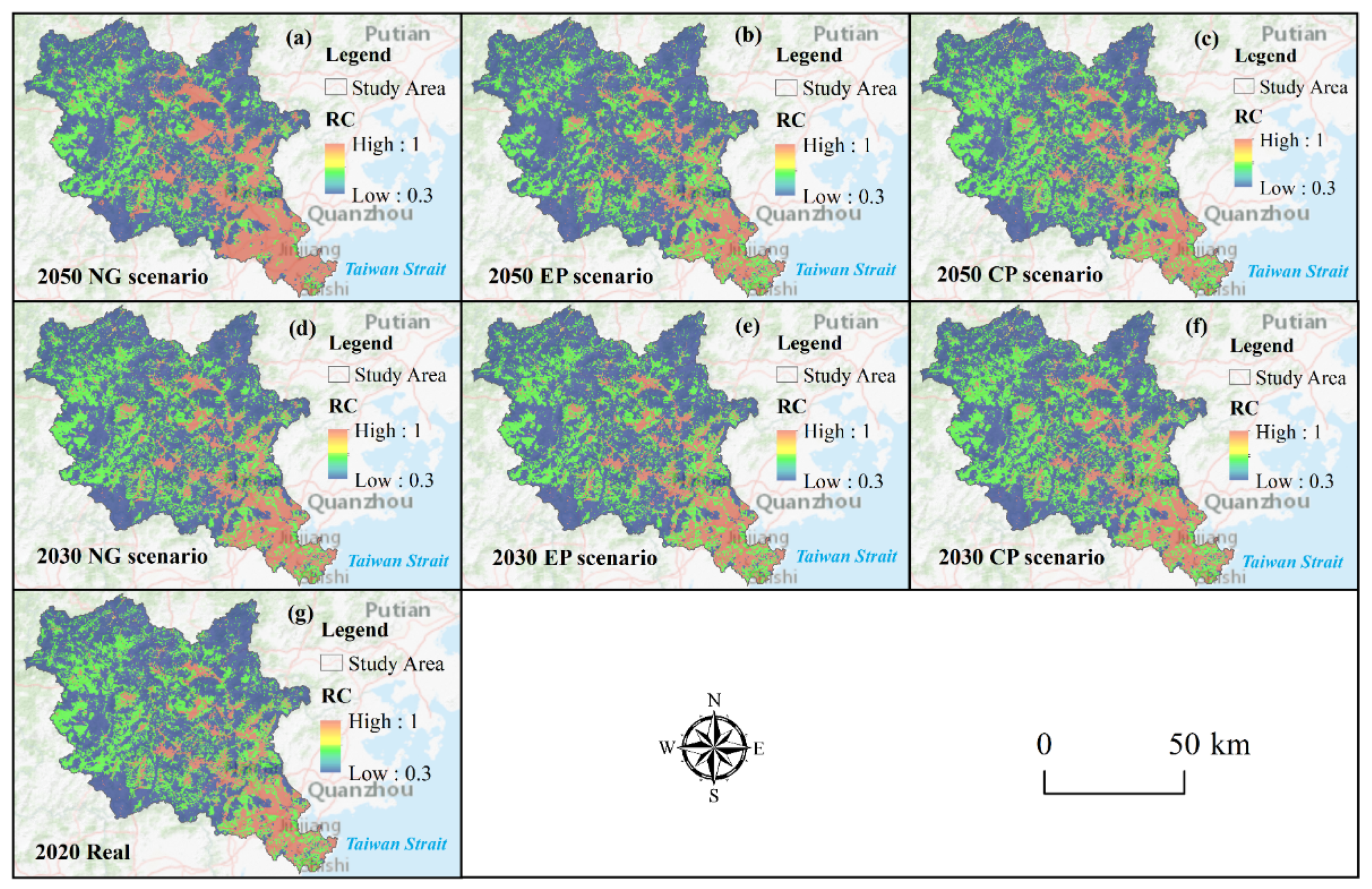
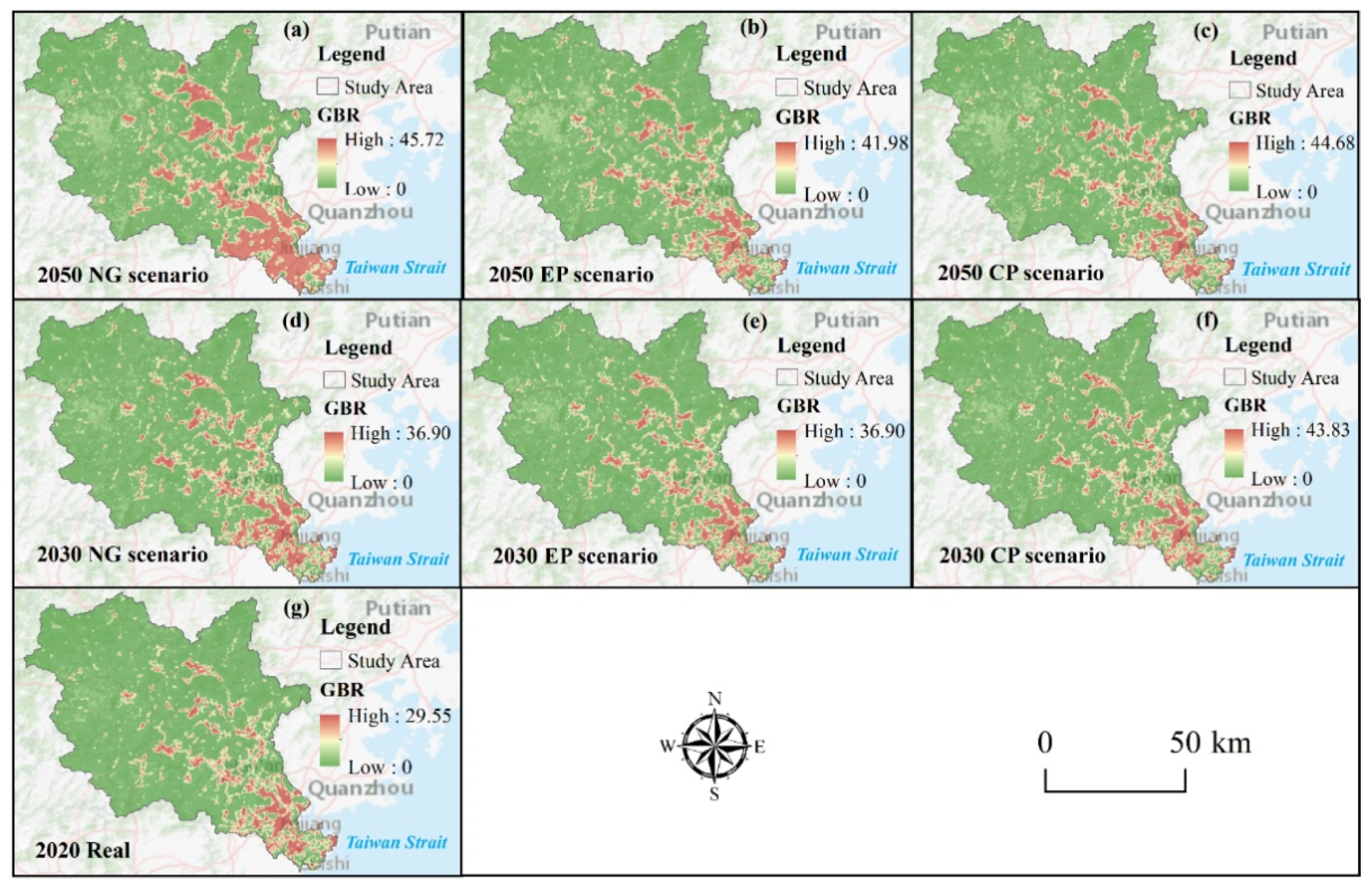
4.2. The Spatialization Results of the Epigenetic Variables
4.3. Spatio-Temporal Characteristics of Future Flood Risk
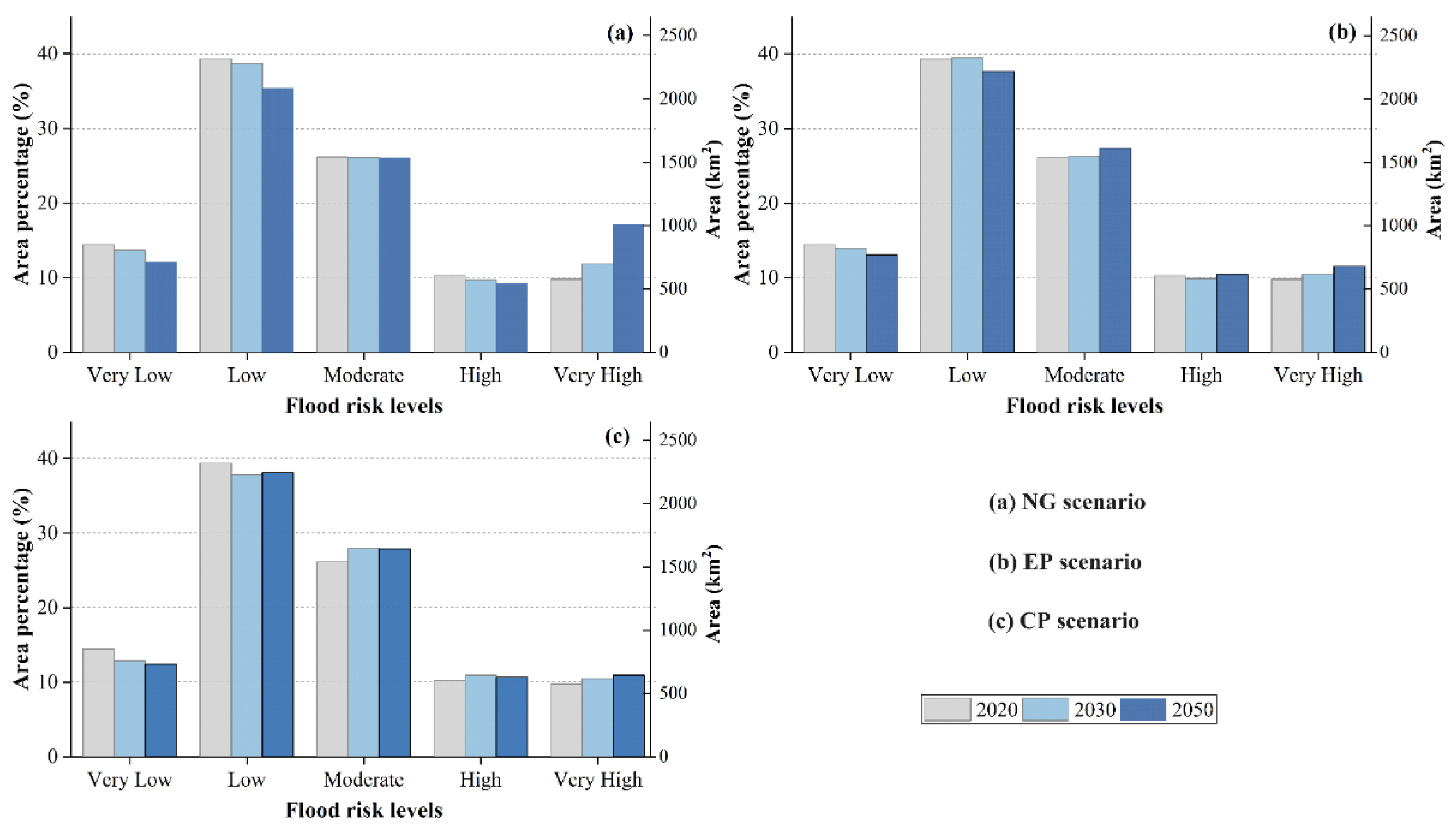
4.3.1. Temporal Patterns of the Flood Risk
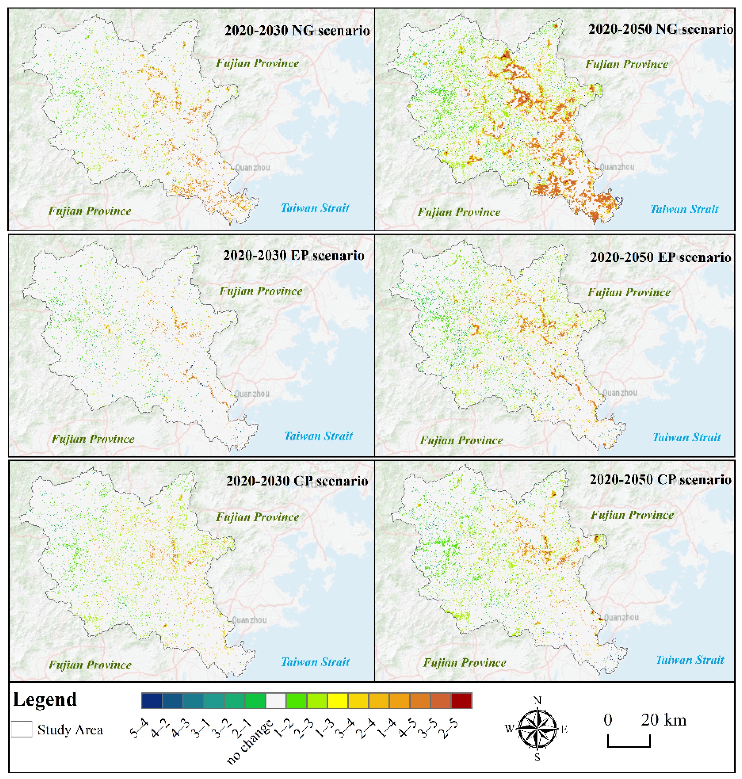
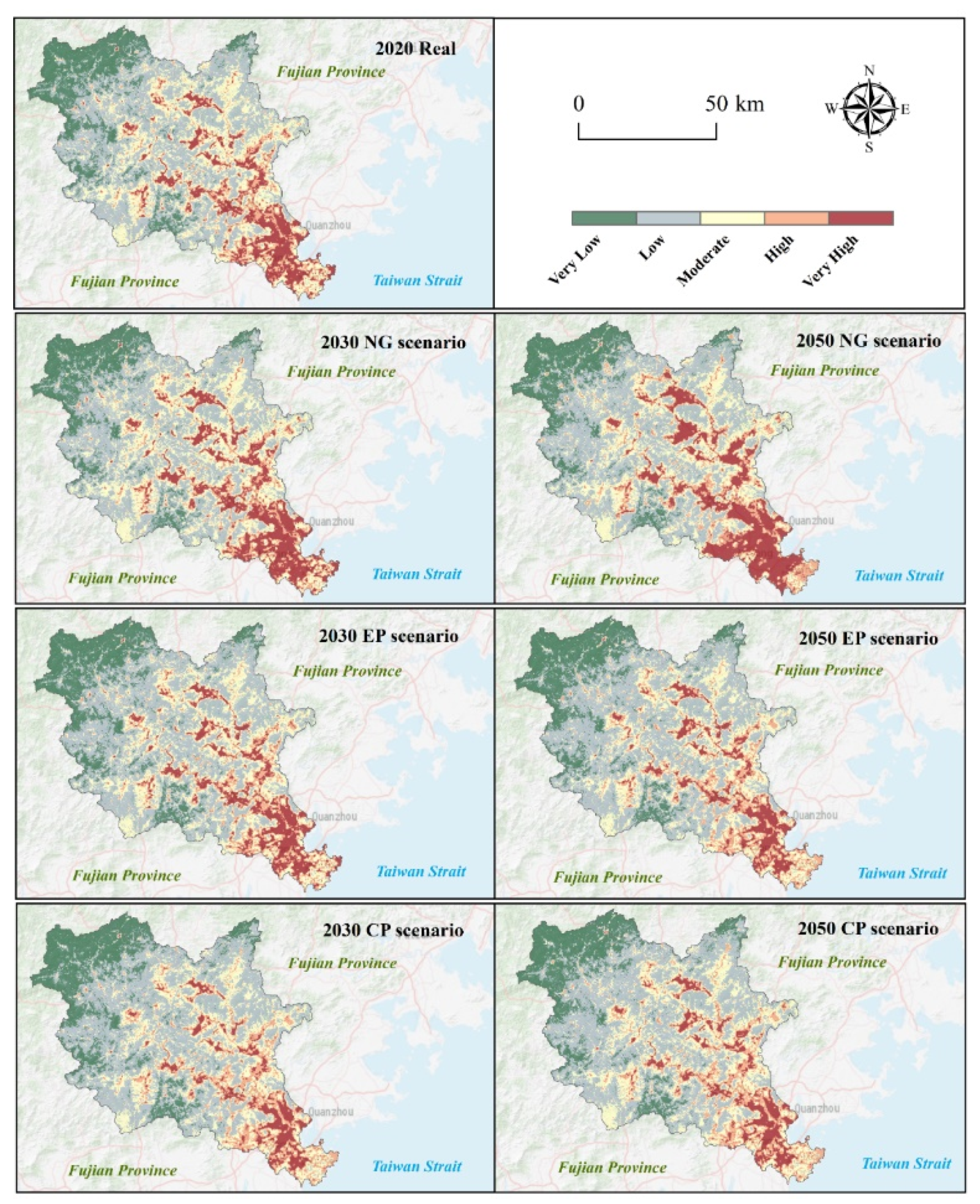
4.3.2. Spatial Patterns of the Flood Risk
5. Discussion
5.1. Analysis of Simulation Results
5.2. Applications and Uncertainty of the Framework
6. Conclusions
Supplementary Materials
Author Contributions
Funding
Institutional Review Board Statement
Informed Consent Statement
Data Availability Statement
Conflicts of Interest
References
- Hong, H.Y.; Tsangaratos, P.; Ilia, I.; Liu, J.Z.; Zhu, A.X.; Chen, W. Application of fuzzy weight of evidence and data mining techniques in construction of flood susceptibility map of Poyang County, China. Sci. Total Environ. 2018, 625, 575–588. [Google Scholar] [CrossRef] [PubMed]
- Dano, U.L.; Balogun, A.L.; Matori, A.N.; Yusouf, K.W.; Abubakar, I.R.; Mohamed, M.A.S.; Aina, Y.A.; Pradhan, B. Flood Susceptibility Mapping Using GIS-Based Analytic Network Process: A Case Study of Perlis, Malaysia. Water 2019, 11, 615. [Google Scholar] [CrossRef] [Green Version]
- Khosravi, K.; Nohani, E.; Maroufinia, E.; Pourghasemi, H.R. A GIS-based flood susceptibility assessment and its mapping in Iran: A comparison between frequency ratio and weights-of-evidence bivariate statistical models with multi-criteria decision-making technique. Nat. Hazards 2016, 83, 947–987. [Google Scholar] [CrossRef]
- Leskens, J.G.; Brugnach, M.; Hoekstra, A.Y.; Schuurmans, W. Why are decisions in flood disaster management so poorly supported by information from flood models? Environ. Model. Softw. 2014, 53, 53–61. [Google Scholar] [CrossRef]
- Yu, F.L.; Chen, Z.Y.; Ren, X.Y.; Yang, G.F. Analysis of historical floods on the Yangtze River, China: Characteristics and explanations. Geomorphology 2009, 113, 210–216. [Google Scholar] [CrossRef]
- Lai, C.G.; Chen, X.H.; Wang, Z.L.; Yu, H.J.; Bai, X.Y. Flood Risk Assessment and Regionalization from Past and Future Perspectives at Basin Scale. Risk Anal. 2020, 40, 1399–1417. [Google Scholar] [CrossRef]
- Costache, R.; Pham, Q.B.; Avand, M.; Linh, N.T.T.; Vojtek, M.; Vojtekova, J.; Lee, S.; Khoi, D.N.; Nhi, P.T.T.; Dung, T.D. Novel hybrid models between bivariate statistics, artificial neural networks and boosting algorithms for flood susceptibility assessment. J. Environ. Manag. 2020, 265, 110485. [Google Scholar] [CrossRef]
- Nachappa, T.G.; Piralilou, S.T.; Gholamnia, K.; Ghorbanzadeh, O.; Rahmati, O.; Blaschke, T. Flood susceptibility mapping with machine learning, multi-criteria decision analysis and ensemble using Dempster Shafer Theory. J. Hydrol. 2020, 590, 125275. [Google Scholar] [CrossRef]
- Myronidis, D.; Stathis, D.; Sapountzis, M. Post-Evaluation of Flood Hazards Induced by Former Artificial Interventions along a Coastal Mediterranean Settlement. J. Hydrol. Eng. 2016, 21, 05016022. [Google Scholar] [CrossRef]
- Choubin, B.; Moradi, E.; Golshan, M.; Adamowski, J.; Sajedi-Hosseini, F.; Mosavi, A. An ensemble prediction of flood susceptibility using multivariate discriminant analysis, classification and regression trees, and support vector machines. Sci. Total Environ. 2019, 651, 2087–2096. [Google Scholar] [CrossRef]
- Li, F.W.; Wang, L.P.; Zhao, Y. Evolvement rules of basin flood risk under low-carbon mode. Part II: Risk assessment of flood disaster under different land use patterns in the Haihe basin. Environ. Monit. Assess. 2017, 189, 397. [Google Scholar] [CrossRef]
- Liu, J.; Wang, S.Y.; Li, D.M. The Analysis of the Impact of Land-Use Changes on Flood Exposure of Wuhan in Yangtze River Basin, China. Water Resour. Manag. 2014, 28, 2507–2522. [Google Scholar] [CrossRef]
- Lin, W.B.; Sun, Y.M.; Nijhuis, S.; Wang, Z.L. Scenario-based flood risk assessment for urbanizing deltas using future land-use simulation (FLUS): Guangzhou Metropolitan Area as a case study. Sci. Total Environ. 2020, 739, 139899. [Google Scholar] [CrossRef]
- Alfieri, L.; Bisselink, B.; Dottori, F.; Naumann, G.; de Roo, A.; Salamon, P.; Wyser, K.; Feyen, L. Global projections of river flood risk in a warmer world. Earths Future 2017, 5, 171–182. [Google Scholar] [CrossRef]
- Bakker, M.H.N.; Duncan, J.A. Future bottlenecks in international river basins: Where transboundary institutions, population growth and hydrological variability intersect. Water Int. 2017, 42, 400–424. [Google Scholar] [CrossRef]
- Mazzoleni, M.; Bacchi, B.; Barontini, S.; Di Baldassarre, G.; Pilotti, M.; Ranzi, R. Flooding Hazard Mapping in Floodplain Areas Affected by Piping Breaches in the Po River, Italy. J. Hydrol. Eng. 2014, 19, 717–731. [Google Scholar] [CrossRef]
- Tehrany, M.S.; Jones, S.; Shabani, F. Identifying the essential flood conditioning factors for flood prone area mapping using machine learning techniques. Catena 2019, 175, 174–192. [Google Scholar] [CrossRef]
- Muis, S.; Guneralp, B.; Jongman, B.; Aerts, J.; Ward, P.J. Flood risk and adaptation strategies under climate change and urban expansion: A probabilistic analysis using global data. Sci. Total Environ. 2015, 538, 445–457. [Google Scholar] [CrossRef]
- Tehrany, M.S.; Pradhan, B.; Mansor, S.; Ahmad, N. Flood susceptibility assessment using GIS-based support vector machine model with different kernel types. Catena 2015, 125, 91–101. [Google Scholar] [CrossRef]
- Wang, Z.L.; Lai, C.G.; Chen, X.H.; Yang, B.; Zhao, S.W.; Bai, X.Y. Flood hazard risk assessment model based on random forest. J. Hydrol. 2015, 527, 1130–1141. [Google Scholar] [CrossRef]
- Kia, M.B.; Pirasteh, S.; Pradhan, B.; Mahmud, A.R.; Sulaiman, W.N.A.; Moradi, A. An artificial neural network model for flood simulation using GIS: Johor River Basin, Malaysia. Environ. Earth Sci. 2012, 67, 251–264. [Google Scholar] [CrossRef]
- Tehrany, M.S.; Pradhan, B.; Jebur, M.N. Spatial prediction of flood susceptible areas using rule based decision tree (DT) and a novel ensemble bivariate and multivariate statistical models in GIS. J. Hydrol. 2013, 504, 69–79. [Google Scholar] [CrossRef]
- Tehrany, M.S.; Pradhan, B.; Jebur, M.N. Flood susceptibility mapping using a novel ensemble weights-of-evidence and support vector machine models in GIS. J. Hydrol. 2014, 512, 332–343. [Google Scholar] [CrossRef]
- Nachappa, T.G.; Meena, S.R. A novel per pixel and object-based ensemble approach for flood susceptibility mapping. Geomat. Nat. Hazards Risk 2020, 11, 2147–2175. [Google Scholar] [CrossRef]
- Liu, J.F.; Wang, X.Q.; Zhang, B.; Li, J.; Zhang, J.Q.; Liu, X.J. Storm flood risk zoning in the typical regions of Asia using GIS technology. Nat. Hazards 2017, 87, 1691–1707. [Google Scholar] [CrossRef]
- Zou, Q.; Zhou, J.Z.; Zhou, C.; Song, L.X.; Guo, J. Comprehensive flood risk assessment based on set pair analysis-variable fuzzy sets model and fuzzy AHP. Stoch. Environ. Res. Risk Assess. 2013, 27, 525–546. [Google Scholar] [CrossRef]
- Lyu, H.M.; Shen, S.L.; Zhou, A.N.; Zhou, W.H. Flood risk assessment of metro systems in a subsiding environment using the interval FAHP-FCA approach. Sustain. Cities Soc. 2019, 50, 101682. [Google Scholar] [CrossRef]
- Ping, C.; Jian, Z.; Yan, X. Empirical Study on the Influencing Factors of High Technology Industrial Security. Manag. Rev. 2017, 29, 50–61. [Google Scholar]
- Liu, F.; Ma, N. Multicriteria ABC Inventory Classification Using the Social Choice Theory. Sustainability 2020, 12, 182. [Google Scholar] [CrossRef] [Green Version]
- Jun, K.S.; Chung, E.S.; Kim, Y.G.; Kim, Y. A fuzzy multi-criteria approach to flood risk vulnerability in South Korea by considering climate change impacts. Expert Syst. Appl. 2013, 40, 1003–1013. [Google Scholar] [CrossRef]
- Song, L.L.; Liu, F. An improvement in DEA cross-efficiency aggregation based on the Shannon entropy. Int. Trans. Oper. Res. 2018, 25, 705–714. [Google Scholar] [CrossRef]
- An, Y.; Tan, X.C.; Gu, B.H.; Zhu, K.W. Flood risk assessment using the CV-TOPSIS method for the Belt and Road Initiative: An empirical study of Southeast Asia. Ecosyst. Health Sustain. 2020, 6, 1765703. [Google Scholar] [CrossRef]
- Govindan, K.; Khodaverdi, R.; Jafarian, A. A fuzzy multi criteria approach for measuring sustainability performance of a supplier based on triple bottom line approach. J. Clean. Prod. 2013, 47, 345–354. [Google Scholar] [CrossRef]
- Yang, W.C.; Xu, K.; Lian, J.J.; Ma, C.; Bin, L.L. Integrated flood vulnerability assessment approach based on TOPSIS and Shannon entropy methods. Ecol. Indic. 2018, 89, 269–280. [Google Scholar] [CrossRef]
- Zhu, H.G.; Liu, F. A Group-Decision-Making Framework for Evaluating Urban Flood Resilience: A Case Study in Yangtze River. Sustainability 2021, 13, 665. [Google Scholar] [CrossRef]
- Sun, W.C.; Wang, J.; Li, Z.J.; Yao, X.L.; Yu, J.S. Influences of Climate Change on Water Resources Availability in Jinjiang Basin, China. Sci. World J. 2014, 2014, 908349. [Google Scholar] [CrossRef]
- Wu, H.F.; Chen, Y.; Chen, X.W.; Liu, M.B.; Gao, L.; Deng, H.J. A New Approach for Optimizing Rain Gauge Networks: A Case Study in the Jinjiang Basin. Water 2020, 12, 2252. [Google Scholar] [CrossRef]
- Yang, T.H.; Yang, S.C.; Ho, J.Y.; Lin, G.F.; Hwang, G.D.; Lee, C.S. Flash flood warnings using the ensemble precipitation forecasting technique: A case study on forecasting floods in Taiwan caused by typhoons. J. Hydrol. 2015, 520, 367–378. [Google Scholar] [CrossRef]
- Huang, D.; Zhang, L. Assessment of Rainstorm Disaster-causing Force of Flood Risk in Central and Eastern China. In Proceedings of the 7th Annual Meeting of Risk Analysis Council of China Association for Disaster Prevention (RAC-2016), Changsha, China, 4–6 November 2016; pp. 200–205. [Google Scholar]
- Mohamoud, Y.M. Evaluating Manning’s roughness coefficients for tilled soils. J. Hydrol. 1992, 135, 143–156. [Google Scholar] [CrossRef]
- Vojtek, M.; Vojtekova, J. Flood Susceptibility Mapping on a National Scale in Slovakia Using the Analytical Hierarchy Process. Water 2019, 11, 17. [Google Scholar] [CrossRef] [Green Version]
- Costache, R.; Dieu Tien, B. Identification of areas prone to flash-flood phenomena using multiple-criteria decision-making, bivariate statistics, machine learning and their ensembles. Sci. Total Environ. 2020, 712, 136492. [Google Scholar] [CrossRef]
- Chapi, K.; Singh, V.P.; Shirzadi, A.; Shahabi, H.; Bui, D.T.; Pham, B.T.; Khosravi, K. A novel hybrid artificial intelligence approach for flood susceptibility assessment. Environ. Model. Softw. 2017, 95, 229–245. [Google Scholar] [CrossRef]
- Arora, A.; Arabameri, A.; Pandey, M.; Siddiqui, M.A.; Shukla, U.K.; Bui, D.T.; Mishra, V.N.; Bhardwaj, A. Optimization of state-of-the-art fuzzy-metaheuristic ANFIS-based machine learning models for flood susceptibility prediction mapping in the Middle Ganga Plain, India. Sci. Total Environ. 2021, 750, 141565. [Google Scholar] [CrossRef]
- Del Giudice, G.; Padulano, R.; Rasulo, G. Spatial prediction of the runoff coefficient in Southern Peninsular Italy for the index flood estimation. Hydrol. Res. 2014, 45, 263–281. [Google Scholar] [CrossRef] [Green Version]
- Sriwongsitanon, N.; Taesombat, W. Effects of land cover on runoff coefficient. J. Hydrol. 2011, 410, 226–238. [Google Scholar] [CrossRef]
- Hu, S.S.; Cheng, X.J.; Zhou, D.M.; Zhang, H. GIS-based flood risk assessment in suburban areas: A case study of the Fangshan District, Beijing. Nat. Hazards 2017, 87, 1525–1543. [Google Scholar] [CrossRef]
- Dandapat, K.; Panda, G.K. Flood vulnerability analysis and risk assessment using analytical hierarchy process. Modeling Earth Syst. Environ. 2017, 3, 1627–1646. [Google Scholar] [CrossRef]
- Li, X.; Lin, S. Analysis of the Relationship between Local Fiscal Revenue and Economic Growth—Wuhan City, Hubei Province as an Example. Caizhengjiandu 2020, 464, 80–90. [Google Scholar]
- Arsanjani, J.J.; Helbich, M.; Kainz, W.; Boloorani, A.D. Integration of logistic regression, Markov chain and cellular automata models to simulate urban expansion. Int. J. Appl. Earth Obs. Geoinf. 2013, 21, 265–275. [Google Scholar] [CrossRef]
- Lu, R.; Huang, X.; Zhuo, T.; Xiao, S.; Zhao, X.; Zhang, X. Land Use Scenarios Si mulation Based on CLUE-S and Markov Composite Model—A Case Study of Taihu Lake Rim in Jiangsu Province. Sci. Geogr. Sin. 2009, 29, 577–581. [Google Scholar]
- Hu, S.; Chen, L.Q.; Li, L.; Zhang, T.; Yuan, L.N.; Cheng, L.; Wang, J.; Wen, M.X. Simulation of Land Use Change and Ecosystem Service Value Dynamics under Ecological Constraints in Anhui Province, China. Int. J. Environ. Res. Public Health 2020, 17, 4228. [Google Scholar] [CrossRef]
- Liu, X.P.; Liang, X.; Li, X.; Xu, X.C.; Ou, J.P.; Chen, Y.M.; Li, S.Y.; Wang, S.J.; Pei, F.S. A future land use simulation model (FLUS) for simulating multiple land use scenarios by coupling human and natural effects. Landsc. Urban. Plan. 2017, 168, 94–116. [Google Scholar] [CrossRef]
- Dong, N.; You, L.; Cai, W.J.; Li, G.; Lin, H. Land use projections in China under global socioeconomic and emission scenarios: Utilizing a scenario-based land-use change assessment framework. Glob. Environ. Chang. Hum. Policy Dimens. 2018, 50, 164–177. [Google Scholar] [CrossRef]
- Liao, W.L.; Liu, X.P.; Xu, X.Y.; Chen, G.Z.; Liang, X.; Zhang, H.H.; Li, X. Projections of land use changes under the plant functional type classification in different SSP-RCP scenarios in China. Sci. Bull. 2020, 65, 1935–1947. [Google Scholar] [CrossRef]
- Chen, Z.Z.; Huang, M.; Zhu, D.Y.; Altan, O. Integrating Remote Sensing and a Markov-FLUS Model to Simulate Future Land Use Changes in Hokkaido, Japan. Remote Sens. 2021, 13, 2621. [Google Scholar] [CrossRef]
- Liang, X.; Liu, X.P.; Li, X.; Chen, Y.M.; Tian, H.; Yao, Y. Delineating multi-scenario urban growth boundaries with a CA-based FLUS model and morphological method. Landsc. Urban. Plan. 2018, 177, 47–63. [Google Scholar] [CrossRef]
- Lai, Y.; Huang, G.Q.; Chen, S.Z.; Lin, S.T.; Lin, W.J.; Lyu, J.X. Land Use Dynamics and Optimization from 2000 to 2020 in East Guangdong Province, China. Sustainability 2021, 13, 3473. [Google Scholar] [CrossRef]
- Kundu, S.; Mondal, A.; Khare, D.; Hain, C.; Lakshmi, V. Projecting Climate and Land Use Change Impacts on Actual Evapotranspiration for the Narmada River Basin in Central India in the Future. Remote Sens. 2018, 10, 578. [Google Scholar] [CrossRef] [Green Version]
- Myronidis, D.; Ioannou, K. Forecasting the Urban Expansion Effects on the Design Storm Hydrograph and Sediment Yield Using Artificial Neural Networks. Water 2019, 11, 31. [Google Scholar] [CrossRef] [Green Version]
- Gounaridis, D.; Chorianopoulos, I.; Symeonakis, E.; Koukoulas, S. A Random Forest-Cellular Automata modelling approach to explore future land use/cover change in Attica (Greece), under different socio-economic realities and scales. Sci. Total Environ. 2019, 646, 320–335. [Google Scholar] [CrossRef]
- Wang, L. Change and Simulation of Land Use in Longnan City Based on FLUS Model. Master’s Thesis, Northwest Normal University, Lanzhou, China, 2020. [Google Scholar]
- Li, J.Y.; Gong, J.; Guldmann, J.M.; Li, S.C.; Zhu, J. Carbon Dynamics in the Northeastern Qinghai-Tibetan Plateau from 1990 to 2030 Using Landsat Land Use/Cover Change Data. Remote Sens. 2020, 12, 528. [Google Scholar] [CrossRef] [Green Version]
- Wang, L.T.; Wang, S.X.; Zhou, Y.; Liu, W.L.; Hou, Y.F.; Zhu, J.F.; Wang, F.T. Mapping population density in China between 1990 and 2010 using remote sensing. Remote Sens. Environ. 2018, 210, 269–281. [Google Scholar] [CrossRef]
- Zeng, C.Q.; Zhou, Y.; Wang, S.X.; Yan, F.L.; Zhao, Q. Population spatialization in China based on night-time imagery and land use data. Int. J. Remote Sens. 2011, 32, 9599–9620. [Google Scholar] [CrossRef]
- Liao, S.; Sun, J. GIS Based Spatialization of Population Census Data in Qinghai—Tibet Plateau. Acta Geogr. Sin. 2003, 58, 25–33. [Google Scholar] [CrossRef]
- Zheng, Q.; Lyu, H.M.; Zhou, A.N.; Shen, S.L. Risk assessment of geohazards along Cheng-Kun railway using fuzzy AHP incorporated into GIS. Geomat. Nat. Hazards Risk 2021, 12, 1508–1531. [Google Scholar] [CrossRef]
- Liu, H.M.; Zhou, W.H.; Shen, S.L.; Zhou, A.N. Inundation risk assessment of metro system using AHP and TFN-AHP in Shenzhen. Sustain. Cities Soc. 2020, 56, 102103. [Google Scholar] [CrossRef]
- Shi, L.Q.; Qiu, M.; Teng, C.; Wang, Y.; Liu, T.H.; Qu, X.Y. Risk assessment of water inrush to coal seams from underlying aquifer by an innovative combination of the TFN-AHP and TOPSIS techniques. Arab. J. Geosci. 2020, 13, 600. [Google Scholar] [CrossRef]
- Deng, H. Multicriteria analysis with fuzzy pairwise comparison. Int. J. Approx. Reason. 1999, 21, 215–231. [Google Scholar] [CrossRef] [Green Version]
- Diakoulaki, D.; Mavrotas, G.; Papayannakis, L. Determining objective weights in multiple criteria problems: The critic method. Comput. Oper. Res. 1995, 22, 763–770. [Google Scholar] [CrossRef]
- Ding, X.; Zhang, D. K-Means Algorithm Based on Synthetic Weighting of AHP and CRITIC. Comput. Syst. Appl. 2016, 25, 182–186. [Google Scholar] [CrossRef]
- Hwang, C.L.; Yoon, K. Multiple Attribute Decision Making: Methods and Applications; Springer: Berlin/Heidelberg, Germany, 1981. [Google Scholar]
- Mao, N.; Song, M.J.; Deng, S.M. Application of TOPSIS method in evaluating the effects of supply vane angle of a task/ambient air conditioning system on energy utilization and thermal comfort. Appl. Energy 2016, 180, 536–545. [Google Scholar] [CrossRef]
- Liu, W.; Zhan, J.Y.; Zhao, F.; Yan, H.M.; Zhang, F.; Wei, X.Q. Impacts of urbanization-induced land-use changes on ecosystem services: A case study of the Pearl River Delta Metropolitan Region, China. Ecol. Indic. 2019, 98, 228–238. [Google Scholar] [CrossRef]
- Waghwala, R.K.; Agnihotri, P.G. Flood risk assessment and resilience strategies for flood risk management: A case study of Surat City. Int. J. Disaster Risk Reduct. 2019, 40, 101155. [Google Scholar] [CrossRef]
- Wan, L.; Ye, X.; Lee, J.; Lu, X.; Zheng, L. Effects of urbanization on ecosystem service values in a mineral resource-based city. Habitat Int. 2015, 46, 54–63. [Google Scholar] [CrossRef]
- Hu, S.; Chen, L.Q.; Li, L.; Wang, B.Y.; Yuan, L.N.; Cheng, L.; Yu, Z.Q.; Zhang, T. Spatiotemporal Dynamics of Ecosystem Service Value Determined by Land-Use Changes in the Urbanization of Anhui Province, China. Int. J. Environ. Res. Public Health 2019, 16, 5104. [Google Scholar] [CrossRef] [Green Version]
- Zhang, X.; Li, A.; Nan, X.; Lei, G.; Wang, C. Multi-scenario Simulation of Land Use Change Along China-Pakistan Economic Corridor through Coupling FLUS Model with SD Model. J. Geo-Inf. Sci. 2020, 22, 17. [Google Scholar]
- Villarreal-Rosas, J.; Wells, J.A.; Sonter, L.J.; Possingham, H.P.; Rhodes, J.R. The impacts of land use change on flood protection services among multiple beneficiaries. Sci. Total Environ. 2022, 806, 150577. [Google Scholar] [CrossRef]
- Rounsevell, M.D.A.; Metzger, M.J. Developing qualitative scenario storylines for environmental change assessment. Wiley Interdiscip. Rev. Clim. Chang. 2010, 1, 606–619. [Google Scholar] [CrossRef]
- Szwagrzyk, M.; Kaim, D.; Price, B.; Wypych, A.; Grabska, E.; Kozak, J. Impact of forecasted land use changes on flood risk in the Polish Carpathians. Nat. Hazards 2018, 94, 227–240. [Google Scholar] [CrossRef] [Green Version]
- Greeuw, S.; Asselt, M.V.; Grosskurth, J. Cloudy Crystal Balls: An Assessment of Recent European and Global Scenario Studies and Models; European Environment Agency: Copenhagen, Denmark, 2000. [Google Scholar]
- Murray-Rust, D.; Rieser, V.; Robinson, D.T.; Milicic, V.; Rounsevell, M. Agent-based modelling of land use dynamics and residential quality of life for future scenarios. Environ. Model. Softw. 2013, 46, 75–89. [Google Scholar] [CrossRef]
- Thieken, A.H.; Cammerer, H.; Dobler, C.; Lammel, J.; Schoberl, F. Estimating changes in flood risks and benefits of non-structural adaptation strategies—A case study from Tyrol, Austria. Mitig. Adapt. Strateg. Glob. Chang. 2016, 21, 343–376. [Google Scholar] [CrossRef] [Green Version]
- Tellman, B.; Saiers, J.E.; Cruz, O.A.R. Quantifying the impacts of land use change on flooding in data-poor watersheds in El Salvador with community-based model calibration. Reg. Environ. Chang. 2016, 16, 1183–1196. [Google Scholar] [CrossRef]
- Huong, H.T.L.; Pathirana, A. Urbanization and climate change impacts on future urban flooding in Can Tho city, Vietnam. Hydrol. Earth Syst. Sci. 2013, 17, 379–394. [Google Scholar] [CrossRef] [Green Version]
- Rapalo, L.M.C.; Uliana, E.M.; Moreira, M.C.; da Silva, D.D.; Ribeiro, C.B.D.; da Cruz, I.F.; Pereira, D.D. Effects of land-use and -cover changes on streamflow regime in the Brazilian Savannah. J. Hydrol. Reg. Stud. 2021, 38, 100934. [Google Scholar] [CrossRef]


| Data Aspect | Sub-Factors | Data | Time | Source of Data | Resolution |
|---|---|---|---|---|---|
| Disaster-inducing factors | M3DP | GPM | 2000–2020 | National Aeronautics and Space Administration (https://disc.gsfc.nasa.gov/datasets/GPM_3IMERGDE_06/summary?keywords=GPM) (accessed on 18 April 2021) | 0.1° × 0.1° |
| R50 mm | |||||
| Disaster-breeding environments | DEM | DEM | 2010 | Geospatial Data Cloud (www.gscloud.cn) (accessed on 6 May 2021) | 30 m × 30 m |
| Slope | |||||
| TWI | |||||
| DR | River | 2013 | National Flash Flood Investigation and Evaluation Project (NFFIEP) | 1:1,000,000 | |
| RC | Land-use | 2020 | Globeland30 (http://www.globeland30.com/) (accessed on 20 May 2021) | 30 m × 30 m | |
| Hazard-bearing bodies | POP | Quanzhou statistical yearbook | 2020 | Quanzhou Statistical Information network (http://tjj.quanzhou.gov.cn/tjzl/tjsj/ndsj/) (accessed on 1 June 2021) | \ |
| GBR |
| Land-Use Type | Cropland | Woodlands | Grassland | Water Area | Built-Up Land | Unused Land |
|---|---|---|---|---|---|---|
| Runoff coefficient | 0.60 | 0.3 | 0.35 | 1.00 | 0.92 | 0.7 |
| Year | Scenario | Cropland | Woodland | Grassland | Water Area | Built-Up Land | Unused Land |
|---|---|---|---|---|---|---|---|
| 2020 | / | 173,528 | 250,238 | 75,297 | 6746 | 81,268 | 484 |
| 2030 | NG | 162,957 | 235,043 | 88,627 | 8364 | 91,944 | 623 |
| EP | 162,957 | 243,227 | 89,995 | 8364 | 82,393 | 623 | |
| CP | 175,565 | 232,285 | 88,627 | 7974 | 82,485 | 623 | |
| 2050 | NG | 134,735 | 212,102 | 108,011 | 11,322 | 120,543 | 848 |
| EP | 146,668 | 230,356 | 114,399 | 10,673 | 84,592 | 873 | |
| CP | 179,905 | 201,947 | 109,825 | 9993 | 85,013 | 878 |
| Variables | 2020 | 2030 | 2050 | ||||
|---|---|---|---|---|---|---|---|
| NG | EP | CP | NG | EP | CP | ||
| POP | 4.23 | 4.68 | 4.48 | 4.55 | 5.44 | 4.78 | 4.97 |
| AAGR | / | 1.02% | 0.57% | 0.73% | 1.27% | 0.61% | 0.80% |
| GBR | 13.86 | 23.18 | 20.67 | 20.50 | 33.20 | 23.43 | 23.07 |
| AAGR | / | 5.28% | 4.08% | 3.99% | 4.46% | 2.66% | 2.58% |
Publisher’s Note: MDPI stays neutral with regard to jurisdictional claims in published maps and institutional affiliations. |
© 2021 by the authors. Licensee MDPI, Basel, Switzerland. This article is an open access article distributed under the terms and conditions of the Creative Commons Attribution (CC BY) license (https://creativecommons.org/licenses/by/4.0/).
Share and Cite
Liu, J.; Wang, J.; Xiong, J.; Cheng, W.; Cui, X.; He, W.; He, Y.; Duan, Y.; Yang, G.; Wang, N. Dynamic Assessment of the Flood Risk at Basin Scale under Simulation of Land-Use Scenarios and Spatialization Technology of Factor. Water 2021, 13, 3239. https://doi.org/10.3390/w13223239
Liu J, Wang J, Xiong J, Cheng W, Cui X, He W, He Y, Duan Y, Yang G, Wang N. Dynamic Assessment of the Flood Risk at Basin Scale under Simulation of Land-Use Scenarios and Spatialization Technology of Factor. Water. 2021; 13(22):3239. https://doi.org/10.3390/w13223239
Chicago/Turabian StyleLiu, Jun, Jiyan Wang, Junnan Xiong, Weiming Cheng, Xingjie Cui, Wen He, Yufeng He, Yu Duan, Gang Yang, and Nan Wang. 2021. "Dynamic Assessment of the Flood Risk at Basin Scale under Simulation of Land-Use Scenarios and Spatialization Technology of Factor" Water 13, no. 22: 3239. https://doi.org/10.3390/w13223239
APA StyleLiu, J., Wang, J., Xiong, J., Cheng, W., Cui, X., He, W., He, Y., Duan, Y., Yang, G., & Wang, N. (2021). Dynamic Assessment of the Flood Risk at Basin Scale under Simulation of Land-Use Scenarios and Spatialization Technology of Factor. Water, 13(22), 3239. https://doi.org/10.3390/w13223239