Comparison of Three Daily Rainfall-Runoff Hydrological Models Using Four Evapotranspiration Models in Four Small Forested Watersheds with Different Land Cover in South-Central Chile

Abstract

We used the lumped rainfall–runoff hydrologic models Génie Rural à 4, 5, 6 paramètres Journalier (GR4J, GR5J and GR6J) to evaluate the most robust model for simulating discharge on four forested small catchments (<40 ha) in south-central Chile. Different evapotranspiration methods were evaluated: Oudin, Hargreaves–Samani and Priestley–Taylor. Oudin’s model allows the achievement of the highest efficiencies in the flow simulation. The more sensitive parameters for each model were identified through a Generalized Probability Uncertainty Estimation (GLUE) model. Our results demonstrate that the three hydrological models were capable of efficiently simulating flow in the four study catchments. However, the GR6J model obtained the most satisfactory results in terms of simulated to measured streamflow closeness. In general, the three models tended to underestimate peak flow, as well as underestimate and overestimate flow events in most of the in situ observations, according to the probability of non-exceedance. We also evaluated the models’ performance in a simulation of summer discharge due to the importance of downstream water supply in the months of greatest scarcity. Again, we found that GR6J obtained the most efficient simulations.

1. Introduction

There is global concern about how the decreased precipitation and increased temperatures associated with climate change will affect water availability [1,2]. There is also the potential for land use and management to amplify the effects of climate change on water resources [3]. Since 2010, Chile has experienced its longest drought on record, and this has been characterized by decreasing precipitation and increasing air temperatures [4,5]. This drought has increased water scarcity in central Chile [6], where most of the plantations and native forest are concentrated and where most of the population lives (34° to 40° S) [7].

To estimate and characterize streamflow, which is used for drinking water and irrigation, among other uses, the application of models fed by hydrometeorological data has been proposed by several authors (e.g., [8,9,10]). Hydrological models can give a better understanding of the role of components in the hydrological cycle in each catchment, in addition to serving as a basis for the modeling of other hydrological processes. Thus, hydrological modeling at the catchment scale is justified [11]. Additionally, at small catchment scales, water availability for human consumption and irrigation is a main concern of society, especially rural communities. Therefore, it is important to know the response of the hydrological regime to both natural and human causes at catchment scale (<100 ha) [12].

The predictive capacity of a hydrological model depends on its structure, the input data quality and resolution in time and space, how and where it is applied and its prediction quality. Modelers usually look for consistency between the understanding of the hydrological system and the model that it represents [13]. Each catchment study has a unique combination of climate, topography, geology and land use [11]. Therefore, hydrological rainfall–runoff models are tools widely used by hydrologists for streamflow estimation [14,15,16,17,18]. There are many hydrological rainfall–runoff models, but the main classifications are conceptual or physically based, and lumped or distributed models [19]. Physical models are usually more complex and require more input data, which is a problem in data-scarce regions (e.g., [20]), so conceptual models have gained attention regarding their simplicity, low amount of data and fewer input variables, but with good representation of streamflow (e.g., [21]).

Some of the conceptual and lumped hydrological models that are currently used are the GR4J—“Génie Rural à 4 paramètres Journalier”—model [22], the GR5J—“Génie Rural à 5 paramètres Journalier”—model [23], the GR6J—“Génie Rural à 6 paramètres Journalier”—model [24], the HYMOD (Hydrologic Model) [25] and the HBV hydrological model [26]. A catchment is represented as one pixel with different buckets or compartments [27]. Models’ inputs are precipitation, temperature and/or potential or actual evapotranspiration. The GR model family (i.e., GR4J, GR5J and GR6J) has been recognized as a family of simple yet robust hydrological models [28,29], and they have been used in several studies around the globe [30,31,32,33,34]. In north-central Chile, for example, Barría et al. used the GR2M model (monthly time step) to model 87 catchments [35]. Refs. [36,37] used the GR4J model in Andean catchments and in the Elqui River in northern Chile, respectively. Ref. [38] showed satisfactory results applying the GR6J model in an Andean catchment in northern Chile [38]. However, within forested/afforested small catchments with different land uses, these models have not yet been applied in Chile.

The minimum information to calibrate hydrological models is streamflow, preferably at the catchment outlet and ideally at sub catchments, precipitation and an estimate of potential evapotranspiration. It is important to note that model performance depends on the quality of the input data, model structure and measurements of model outputs [39]. While streamflow, precipitation and temperature data are often available, potential evapotranspiration has multiple ways of calculation (i.e., [40,41,42]), so it poses a challenge given the numerous approaches to its estimation [43]. In this regard, there are several types of potential evapotranspiration methods/models available, which can be classified as: (i) fully physically based combination models; (ii) semi physically based models; and (iii) black-box models based on artificial neural networks (e.g., [44]), empirical relationships and fuzzy and genetic algorithms for calibration and parameters’ optimization [45]. For example, some approaches to potential evapotranspiration (PET) and actual evapotranspiration (AET) estimation are derived from remote sensing products, but they need to be calibrated with ground data (e.g., [46]), which are not always available.

The most common approach to estimate PET (the water released to the atmosphere by soil and plants under no water stress) is empirical relationships between temperature and other meteorological variables such as wind speed and radiation [40]. As meteorological data are usually limited in remote areas and in small catchments, remote sensing information has been used (e.g., [47]). However, since they do not have observed values, PET/AET estimation is challenging [43]. Ref. [48] showed that formulae based on temperature and radiation tend to provide the best streamflow simulations. PET estimates based on the Penman approach [49] seem less suited to use in rainfall–runoff models [48]. However, a complex PET approach does not guarantee better results compared to a simplistic approach [48]. Additionally, the forest potential evapotranspiration (PET) and actual evapotranspiration (AET) vary spatially and temporally. The former depends on the atmospheric capability to absorb water stream, while the latter depends on the vegetation characteristics, silvicultural practices and abiotic characteristics such as climate and water availability [50].

Some authors recommend using PET models based on temperature [51,52], while others consider the physical processes in evapotranspiration with an eddy covariance analysis evaluating the transformation between AET and PET and its application in conceptual hydrological models [53]. However, the gap on this issue is still in development because meteorological information is still scarce, and particularly in the coastal range of Chile [54]. For instance, the Priestley–Taylor AET equation, a simplified form of the Penman–Monteith model, has been widely used for humid regions [55]. Thus, the model proposed by [55] not only considers meteorological variables for the estimation of actual evapotranspiration, but also adds a factor related to vegetation in the study area, with the objective of making a more realistic estimate of evapotranspiration. The importance of knowing AET and PET is that changes under climate change may affect streamflow yield in the future, impacting water security [56].

Different evapotranspiration models and hydrological models have been used for flow simulation. Ref. [57] reviewed different methods for estimating evapotranspiration in hydrological models. For instance, ref. [58] used the SWAT hydrological model in conjunction with the Penman–Monteith, Hargreaves and Priestley–Taylor evapotranspiration models for flow simulation in northern Tunisia, where they observed that streamflow simulation was not significantly affected by the PET estimation used. Ref. [59] used the hydrological model SWAT-2000 along with Hargreaves and Penman–Monteith evapotranspiration models for the simulation of flow on a small catchment in Bedfordshire, England and also used the infiltration methods NRCS curve number (CN) and Green and Ampt for runoff estimation, showing that different combinations of PET and runoff models are necessary to identify their contribution to the simulation quality of hydrological models.

In Chile, ref. [60] used the Hargreaves–Samani method for PET calculation within a land use change model simulation with SWAT in central-southern Chile. Refs. [54,61] used the Hargreaves–Samani PET equation in a runoff ratio analysis in small catchments in south-central Chile and several catchments across Chile, respectively. Ref. [62] used the SWEAP hydrological model with Hargreaves–Samani PET for planning an expansion of irrigated areas in the north-eastern area of the Araucanía region. Although there is increasing research about PET/AET estimation in Chile, very few studies have been applied in small catchments (e.g., [61]), and as far as we know, none compared different PET/AET methods in hydrological modeling.

Many factors must be considered when determining which precipitation–runoff hydrological model to use within the study catchment. In large and highly heterogeneous catchments, a more complex hydrological model that considers a high number of input variables and parameters results in higher quality simulation [63,64]. In the case of small catchments, spatial variability is lower, requiring less complex models to provide satisfactory results [65]. Moreover, authors such as [66] have not observed significant differences in the quality of simulation of models of different complexities for similar scenarios. In addition, the hydrological parameters that define each model do not necessarily have the same weight in the output. There are parameters that highly influence the behavior of the model, while others influence the behavior minimally [67]. This implies the need for a sensitivity analysis to identify the relative dominance of each parameter in the hydrological model that is used. In addition, the different evapotranspiration models, having different considerations, yield different evapotranspiration values. This generates distinct input values for each hydrological precipitation runoff model, so that finally, flow simulations rely on the forcing evapotranspiration model.

Our working hypotheses are: (1) increasing model complexity will allow for greater efficiency in simulating discharge in small catchments; and (2) a tentative suggestion is made regarding a possible role for potential evapotranspiration in the forest environment. Therefore, the objective of this study was to investigate the GR lumped daily hydrological models’ family performance in four forested catchments across different PET approaches (PET and AET) and how the PET/AET approaches impact the modeling of small catchments and model complexity. We achieved this by analyzing (a) annual streamflow, (b) summer flows and (c) peak flows on these four catchments in south-central Chile.

This paper is organized as follows: (i) introduction to flow simulation using different hydrological and evapotranspiration models; (ii) methodology that describes the study area, hydrological, PET and AET models, efficiency statistics, calibration and validation periods and sensitivity analysis; (iii) results showing the evapotranspiration methods and parameter sets that maximize the efficiency of hydrological models, the quality of the simulation, annual hydrograph analysis and minimum flows and the sensitivity of the parameters through the GLUE method; (iv) summary of the main results and possible extensions of this work; (v) conclusions; and (vi) appendix with graphical representation of the sensitivity of the parameters in the hydrological models GR4J, GR5J and GR6J.

2. Materials and Methods

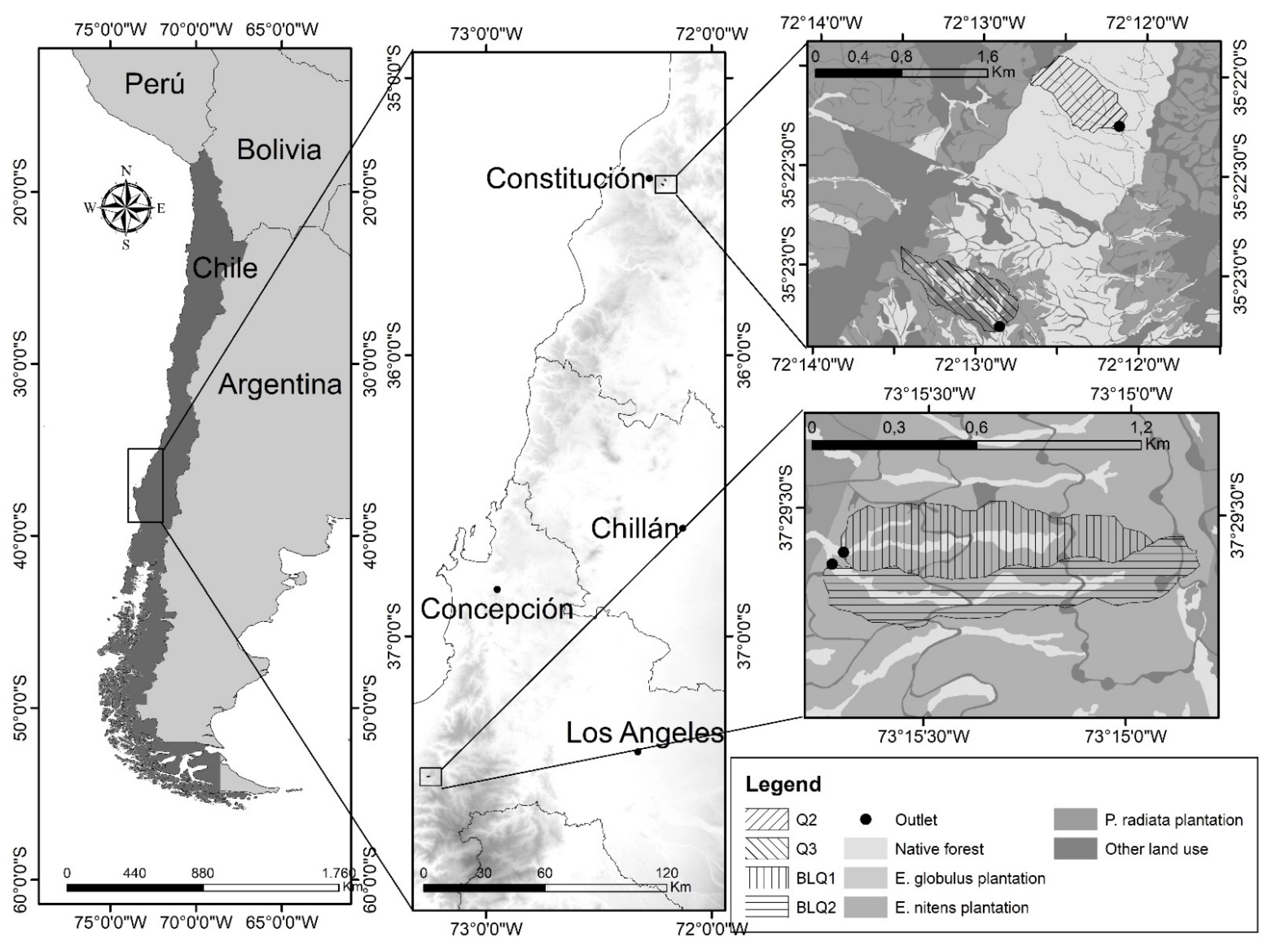
2.1. Study Area

The study area comprised four coastal catchments in south-central Chile: Quivolgo 2 (Q2), Quivolgo 3 (Q3), Bajo las Quemas 1 (BLQ1) and Bajo las Quemas 2 (BLQ2). The Quivolgo catchments are located near the city of Constitución (35.20° S), while those of Bajo las Quemas are located near the town of Curanilahue (37.28° S) (Figure 1).

Regarding the climatological characteristics of the catchment, dry months are from November to March, and rainy months are from May to August. All the catchments have a similar intra-annual distribution of precipitation and temperature (Figure 2a,b). Annual precipitation in Q2 and Q3 varied between 727 and 1342 mm over the last 10 years, with a mean annual value of 941.08 mm and a mean daily value of 2.56 mm [68]. In BLQ1 and BLQ2, annual precipitation ranged from 1324 mm to 2146 mm between 2010 and 2016, with a mean annual value of 1698 mm and a mean daily value of 4.65 mm. Average monthly flow reaches its maximum values in the months of July, August and September in the four catchments. BLQ1 exhibited the highest flow values, followed by BLQ2, Q2 and Q3. Minimum average monthly flows are reached in the summer months (January to March) for the four study catchments, specifically in the months of February and March (Figure 2c). Surface, land cover and elevation characteristics are presented in

Table 1. Vegetation cover and geomorphological data of surface (ha), exposure (°) and slope (°) in the catchments.

Catchment	Area	Land Cover	Aspect	Slope
	(ha)		(Grade)	(%)
Q2	33.02	Native forest	135.61	27.33
Q3	40.14	Native forest and P. radiata plantation (Mixed)	179.38	24.13
BLQ1	22.63	E. nitens plantation	309.88	14.71
BLQ2	22.21	E. nitens plantation	285.11	14.15

.

Q2 is covered by Nothofagus glauca (Hualo) as the dominant species, a native and winter deciduous species [68]. Q3 is a mixed catchment covered by Pinus radiata planted in 2001 (62%) and native forest with N. glauca as the main species (34%). BLQ1 and BLQ2 are covered by Eucalyptus nitens plantations with an initial stock density of 1666 trees ha⁻¹; no forest management was performed in these catchments [3].

In Q2 and Q3, soils have originated from metamorphic rocks [3,68] with a topography of hills and ridges, with variable and complex slopes. The soil is shallow, with depths between 0 and 100 cm and organic matter between 3 and 4% on the surface [69], and is composed of silt, clay and sand in the order of 36, 40 and 24%, respectively [68]. The soil has rock fragments, and the subsoil rock is dominated by deep seams of partially weathered material [68]. Soils of BLQ1 and BLQ2 have their origin in the group of metamorphic soils that have been formed from material generating shales, sandstones, phyllites and schists [69]. Usually, these soils have clay textures, low water infiltration and occupy positions that vary from abrupt hills and mountain ranges with variable and complex slopes. They present a physiography of mountains dissected by deep ravines, mountainous topography, good external drainage, moderate internal drainage and parent material composed of shales [69].

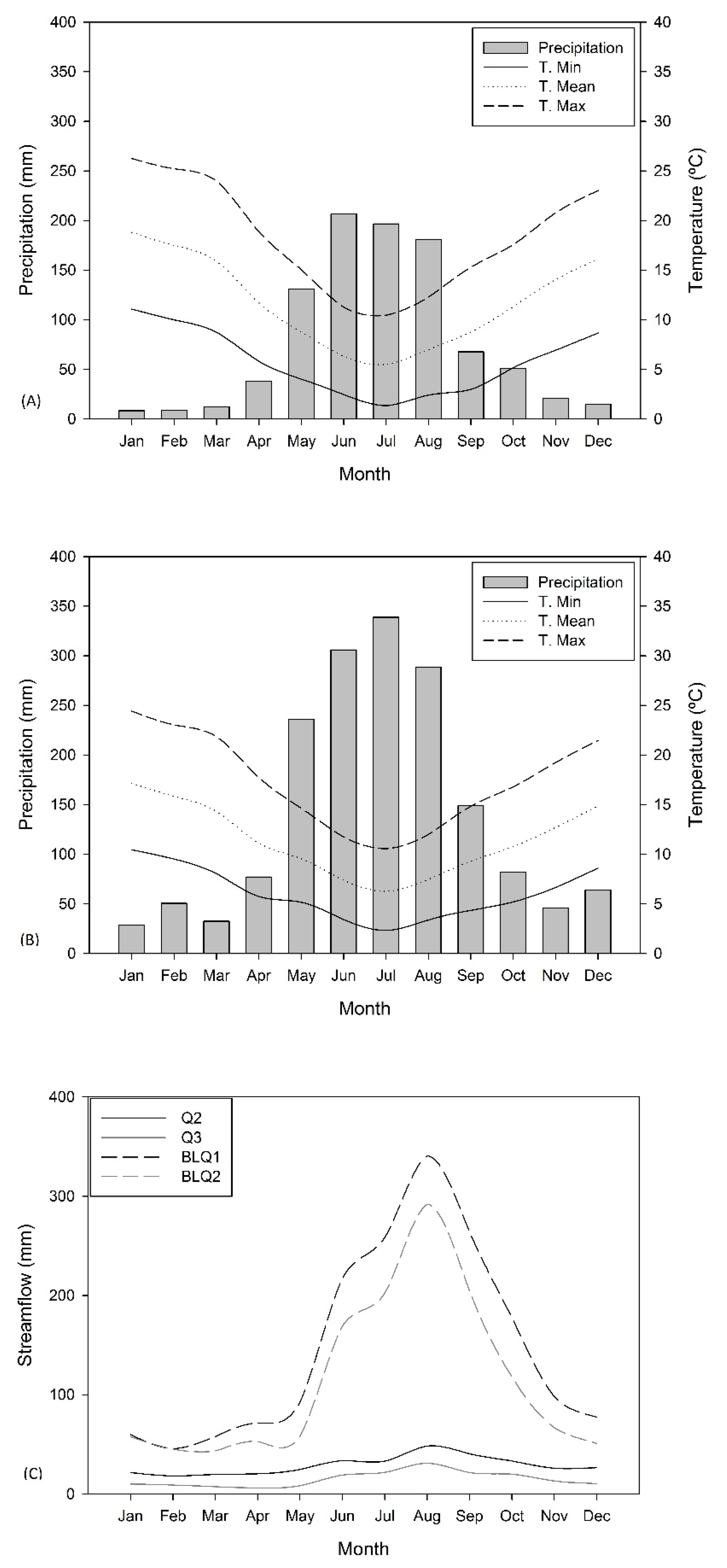
2.2. Hydrometeorological Data

To obtain meteorological data in Q2 and Q3, a tipping-bucket automatic rain gauge (Environdata Weather Stations Pty Ltd., Australia) was installed 35 m north of Q2 headwater and 2.3 km north of Q3 to obtain hourly temperature and precipitation data (Figure 1). Rainfall measurements commenced in August 2016. For the period between 2010 and August 2016 (when streamflow data are available), daily rainfall was sourced from the nearby meteorological site (Forel station, ‘Dirección General de Aguas’, DGA), which is about 5 km south-east of the catchment (for more information, see [68]). For BLQ1 and BLQ2, a daily rain gauge station was used, installed 11 km to the northwest of the catchments.

For discharge estimation, a 90° V-notch weir was built at all catchment outlets. Water height at the weir was measured with a pressure transducer (KPSI (Q2 and Q3), OTT (Q2 Aug-2014, BLQ1 and BLQ2)) and discharge was estimated every 5 min from the theoretic rating curve for each weir [3]. Discharge records were available from 2009 in Q2 and from 2013 in Q3, BLQ1 and BLQ2.

Finally, net radiation was calculated from climatological data such as minimum and maximum temperature and geomorphological data such as exposure and slope available around nearby weather stations [70].

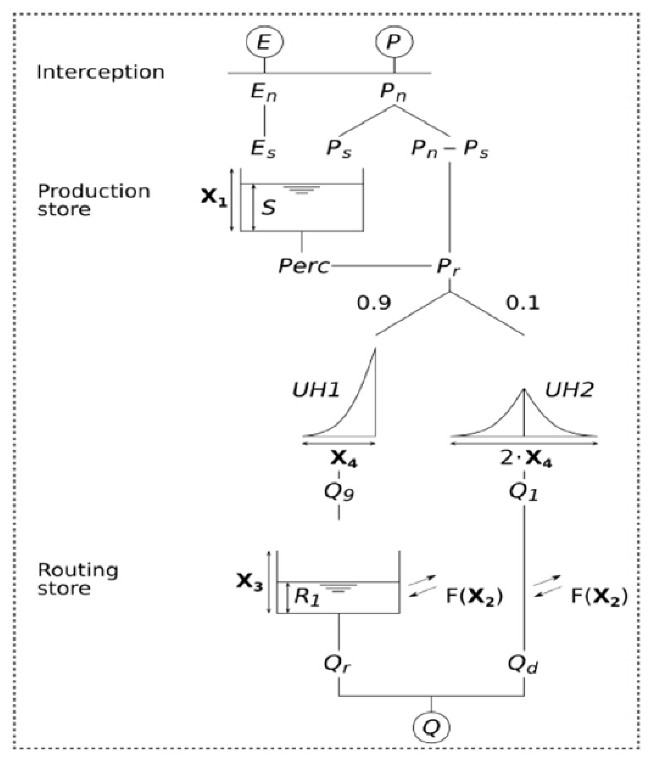
2.3. Hydrological Models

The GR4J, GR5J and GR6J rainfall–runoff hydrologic models were used to simulate annual and peak flows and summer discharge in four small catchments in south-central Chile. These models were selected as they have been used in several catchments with a reasonable performance (e.g., [71,72]).

They have been described as metric-conceptual, deterministic and grouped models for daily runoff data using four, five and six parameters, respectively. These models belong to the family of soil moisture models, in which the number of parameters is determined by their functionality and parameterization [22]. The models’ input data are daily rainfall (P in mm), daily PET (in mm) and observed streamflow for calibration/validation. Later, with P and PET as input, net rainfall and net evapotranspiration (Pn and Es, respectively, in Figure 3) are calculated. When P is greater than PET, Ps and Pr can be calculated, and available water is routed to storage. These calculations applied to all GRxJ models. More details of the models’ configuration can be found in [22].

The GR4J model employs four parameters—X₁: maximum storage capacity (mm); X₂: groundwater exchange coefficient (mm); X₃: maximum channel transit capacity (mm); and X₄: base time of unit hydrograph (days) [22] (Figure 3).

The GR5J model is a modification of the GR4J model [23]. This modification incorporated an additional parameter intended to consider groundwater exchange between more complex catchments, which can take positive or negative values (dimensionless). The latter parameter, X₅, is an exchange threshold between precipitation capture (dimensionless) [74].

The GR6J model considers an additional parameter that gives a more detailed analysis in the model structure, resulting in a higher quality simulation of low discharge. Thus, the X₆ parameter corresponds to the exponential storage vacuum coefficient and can only take values greater than or equal to 0 [24,74]. A better understanding of the methodological steps followed for this research work is shown in Figure 4.

The airGR package for R software version 3.6.0 [74,75] was used to run these models.

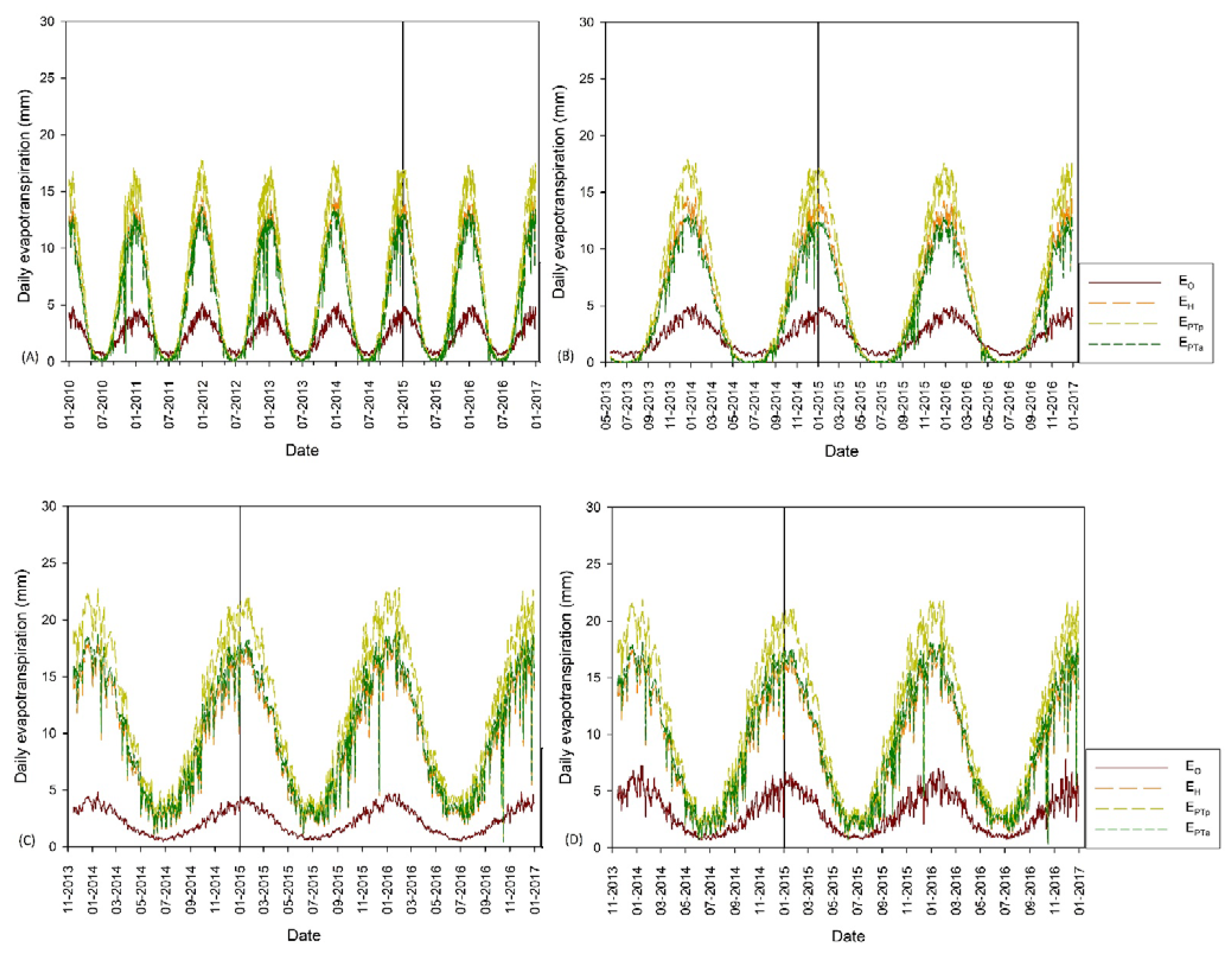
2.4. Evapotranspiration Models

Although input data for the hydrological models are precipitation and potential evapotranspiration, we decided to also use alternative models of AET to verify whether their use is adequate for the hydrological models under study and for forested catchments as the chosen AET model differentiates between land covers. From this comparison, it was possible to determine which model gives a more efficient simulation in each catchment. The models used were the Oudin model [48], Hargreaves–Samani model [76] and Priestley–Taylor model [55].

The Oudin (E_O) model [48] (Equations (1) and (2)) is defined as a physically based daily potential model in which potential evapotranspiration depends exclusively on temperature and extraterrestrial solar radiation.

$$\mathrm{t}+5>0=>{\mathrm{E}}_{\mathrm{O}}=\frac{{\mathrm{R}}_{\mathrm{e}}}{\mathsf{\lambda }\mathsf{\rho }}\frac{\mathrm{t}+5}{100}$$

(1)

$$\mathrm{t}+5\le 0=>{\mathrm{E}}_{\mathrm{O}}=0$$

(2)

where E_O = Oudin’s model estimate for potential evapotranspiration (mm day⁻¹); ${\mathrm{R}}_{\mathrm{e}}$ = extraterrestrial radiation (Mj m² day⁻¹); $\mathrm{t}$ = temperature (°C); $\mathsf{\lambda }$ = latent heat flux (Mj kg⁻¹); $\mathsf{\rho }$ = water density (kg m⁻³).

The Hargreaves–Samani (E_H) model (Equation (3)) is a daily potential evapotranspiration model, also physics-based, which, unlike the one proposed by Oudin, depends on temperature and incident solar radiation [76].

$${\mathrm{E}}_{\mathrm{H}}=0.0135\ast \left(\mathrm{t}+17.78\right)\ast {\mathrm{R}}_{\mathrm{S}}$$

(3)

where E_H = Hargreaves’ model estimate for potential evapotranspiration (mm day⁻¹); R_S = incident radiation (mm day⁻¹); t = temperature (°C).

The Priestley–Taylor model (E_PTp) [55] (Equation (4)) defines potential evaporation as the evaporation that would occur from a hypothetical saturated surface, with similar radiative properties throughout the study area. This area is small enough so that excess moisture flux does not change the characteristics of the convective boundary layer.

$${\mathrm{E}}_{\mathrm{P}\mathrm{T}\mathrm{p}}=\frac{\mathsf{\Delta }}{\mathsf{\Delta }+\mathsf{{\rm Y}}}\left({\mathrm{R}}_{\mathrm{n}}-\mathrm{G}\right)$$

(4)

where E_PTp = equilibrium rate of evapotranspiration (mm day⁻¹), which assumes no aerodynamic transfer; Δ = slope of the saturated steam heat curve (Pa °C⁻¹); Υ = psychometric constant (Pa °C⁻¹); λ = latent heat flux (Mj kg⁻¹).

The equilibrium rate of actual evaporation is modified to give Priestley–Taylor PET as AET = α ∗ E_PTp [77]. The parameter “α” is related to the vegetation land cover and corresponds to the relationship between the rate of evapotranspiration and the rate of limiting evapotranspiration observed in the study area [55].

Thus, a model is obtained of actual evapotranspiration (E_PTa) (Equation (5)). The parameter “α” has been studied by several authors and calculated for different types of ecosystems (e.g., [77,78]). In our case, it was estimated from the values proposed by [79,80,81] for coniferous and broad-leaved temperate forests (0.77 for native forest in Q2, 0.73 for coniferous and native forest in Q3 and 0.83 for broad-leaved eucalyptus in BLQ1 and BLQ2). For more details of E_O, E_H, E_PTp and E_PTa, see [48,76,79,80,81].

$${\mathrm{E}}_{\mathrm{P}\mathrm{T}\mathrm{a}}=\mathsf{\alpha }\frac{\mathsf{\Delta }}{\mathsf{\Delta }+\mathsf{{\rm Y}}}\left({\mathrm{R}}_{\mathrm{n}}-\mathrm{G}\right)$$

(5)

where E_PTa = Priestley–Taylor’s model estimate for actual evapotranspiration (mm day⁻¹); Δ = slope of the saturated steam heat curve (Pa °C⁻¹); Υ = psychometric constant (Pa °C⁻¹); λ = latent heat flux (Mj kg⁻¹); α = coefficient related to vegetation land cover.

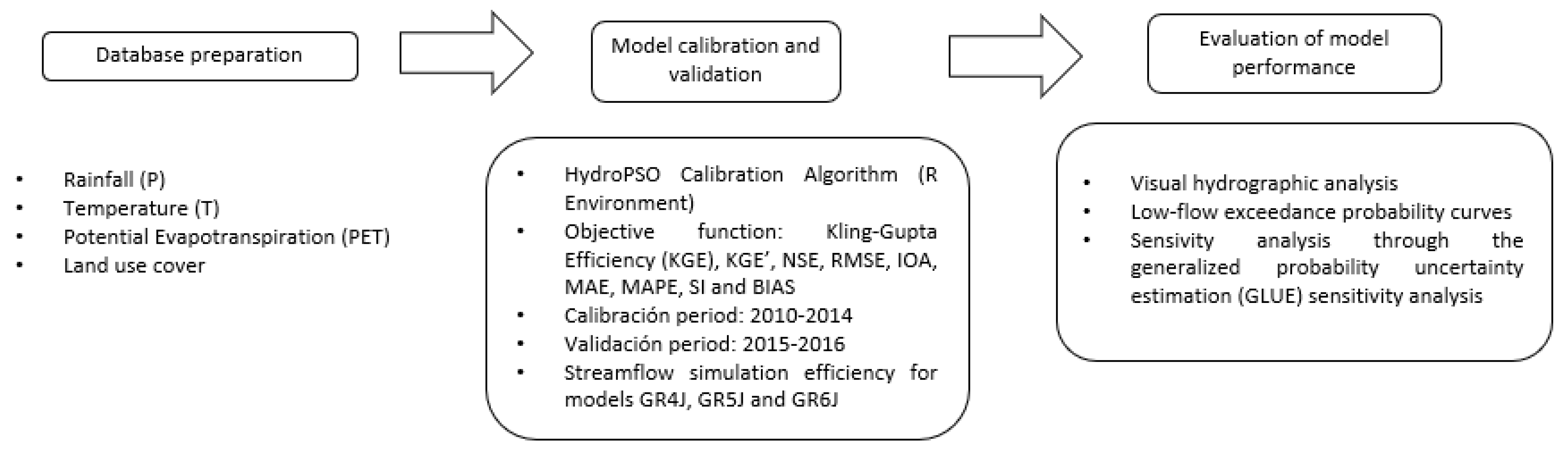
2.5. Model Calibration and Validation

The discharge rate record was divided into two subsamples, one of which is used in the calibration process and the other in the validation [82].

In summer of 2017, a wildfire burned the Q2 and Q3 catchments [68]. As a consequence, the validation period was defined as 1 January 2015 to 31 December 2016 to have the same validation period in all catchments and to isolate the hydrologic effects of the wildfire in the Q2/Q3 catchments. The calibration period is determined by data availability; in Q2 it started from 1 March 2010 to 31 December 2014 and in Q3 from 15 May 2013 to 31 December 2014. In BLQ1 and BLQ2, this period was from 15 November 2013 to 31 December 2014.

The airGR package uses the “Mitchell” calibration algorithm [75] to reach a single set of parameters for each model. This algorithm starts from a global approach in which it considers several initial values for each of the parameters and identifies the initial set that optimizes the simulation quality of the models. Additionally, the methodology proposed by [73] was used for the GR4J model, which uses the previously identified set of parameters as a starting point for its optimization and seeks to maximize the Kling–Gupta statistics (KGE and KGE’) and the Nash–Sutcliffe criterion (NSE).

For the GR5J and GR6J models, a local optimization available in the airGR package was used to complement the Mitchell calibration, which considers the set of parameters previously identified as a starting point for the optimization and seeks to minimize the root mean square error (RMSE).

2.6. Model Efficiency

Discharge simulation performed by each of the models corresponded to a daily time step, so the variation in the observed and simulated daily discharges was evaluated throughout the calibration and validation periods, as well as the summer discharges (December–March). The tools used for the comparison of discharge were mainly hydrographs and exceedance probability curves [83].

Additionally, model efficiency in the calibration and validation periods was evaluated using the Kling–Gupta efficiency criteria (KGE and KGE’) [84], the root mean square error (RMSE) [71], the Nash–Sutcliffe efficiency criterion (NSE) [85], the index of agreement (IOA) [86], the mean absolute error (MAE) [86], the mean absolute percentage error (MAPE) [87], the scatter index (SI) [88] and BIAS [86,89].

For summer flows, the logarithmic version of the NSE criterion was used (NSElog), i.e., it is calculated from the logarithmic values of the simulated and observed data (e.g., [90]) and has the advantage of reducing the influence of maximum flows, while maintaining that of minimum flows [91] (

Table 2. Model efficiency statistics.

N°	Equation	Values	Reference
1	$KGE=1-\sqrt{{\left(1-\alpha \right)}^2+{\left(1-\beta \right)}^2+{\left(1-\rho \right)}^2}$ $\alpha =\frac{{\sigma }_{obs}}{{\sigma }_{sim}}$$;\beta =\frac{{\mu }_{obs}}{{\mu }_{sim}}$	${\sigma }_{obs}=ST observed streamflow$ ${\sigma }_{sim}=ST simulated streamflow$ ${\mu }_{obs}=Mean observed streamflos$ ${\mu }_{sim}=Mean simulated streamflow$ $\rho =Pearson correlation$	[84]
2	$KGE=1-\sqrt{{\left(1-\alpha \right)}^2+{\left(1-\beta \right)}^2+{\left(1-\rho \right)}^2}$ $\alpha =\frac{C{V}_{obs}}{C{V}_{sim}}$$;\beta =\frac{{\mu }_{obs}}{{\mu }_{sim}}$	$C{V}_{obs}=Coefficient of variation observed streamflow$ $C{V}_{sim}=Coefficient of variation simulated streamflow$ ${\mu }_{obs}=Mean observed streamflow$ ${\mu }_{sim}=Mean simulated streamflow$ $\rho =Pearson correlation$	[84]
3	$RMSE=\sqrt{\frac{{{\displaystyle \sum }}_{i=1}^n{\left({\widehat{Q}}_i-Q_i\right)}^2}{n}}$	$Q_i=Observed streamflow$ ${\widehat{Q}}_i=Simulated streamflow$ $n=Data number$	[71]
4	$NSE=1-\left[\frac{{{\displaystyle \sum }}_{i=1}^n{\left({\widehat{Q}}_i-Q_i\right)}^2}{{{\displaystyle \sum }}_{i=1}^n{\left(\overline{Q}-Q_i\right)}^2}\right]$	$Q_i=Observed streamflow$ ${\widehat{Q}}_i=Simulated streamflow$ $\overline{Q}=Mean observed streamflow$	[85]
5	$IOA=1-\frac{{{\displaystyle \sum }}_{i=1}^n{\left({\widehat{Q}}_i-Q_i\right)}^2}{{{\displaystyle \sum }}_{i=1}^n{\left(\left|\overline{Q}-Q_i\right|+\left|\overline{Q}-{\widehat{Q}}_i\right|\right)}^2}$	$Q_i=Observed streamflow$ ${\widehat{Q}}_i=Simulated streamflow$ $\overline{Q}=Mean observed streamflow$ $n=Data number$	[86,87]
6	$MAE=\frac{{{\displaystyle \sum }}_{i=1}^n\left|{\widehat{Q}}_i-Q_i\right|}{n}$	$Q_i=Observed streamflow$ ${\widehat{Q}}_i=Simulated streamflow$ $n=Data number$	[86]
7	$MAPE=\frac{100\ast {{\displaystyle \sum }}_{i=1}^n\left|\frac{{\widehat{Q}}_i-Q_i}{Q_i}\right|}{n}$	$Q_i=Observed streamflow$ ${\widehat{Q}}_i=Simulated streamflow$ $n=Data number$	[87]
8	$SI=\frac{\sqrt{\frac{{{\displaystyle \sum }}_{i=1}^n{\left(\left({\widehat{Q}}_i-{\overline{Q}}_i\right)-\left(Q_i-\overline{Q}\right)\right)}^2}{n}}}{\frac{{{\displaystyle \sum }}_{i=1}^n{Q}_i}{n}}$	$Q_i=Observed streamflow$ ${\widehat{Q}}_i=Simulated streamflow$ $\overline{Q}=Mean observed streamflow$ $\overline{Q_i}=Mean simulated streamflow$ $n=Data number$	[88]
9	$BIAS=\frac{{{\displaystyle \sum }}_{i=1}^n\left({\widehat{Q}}_i-Q_i\right)}{n}$	$Q_i=Observed streamflow$ ${\widehat{Q}}_i=Simulated streamflow$ $n=Data number$	[86,89]
8	$NSElog=1-\left[\frac{{{\displaystyle \sum }}_{i=1}^n\left(log({\widehat{Q}}_i\right)-log\left(Q_i\right){)}^2}{{{\displaystyle \sum }}_{i=1}^n\left(\overline{log(Q}\right)-log(Q_i){)}^2}\right]$	$\log \left(Q_i\right)=Logaritmic observed streamflow$ $log({\widehat{Q}}_i)=Logarithmic simulated streamflow$ $\overline{log\left(Q\right)}=Mean of logarithmic observed streamflow$	[90,91]

). It is important to note that the alpha parameter of the KGE and KGE’ statistics does not correspond to the same alpha parameter used for the calculation of AET (E_PTa).

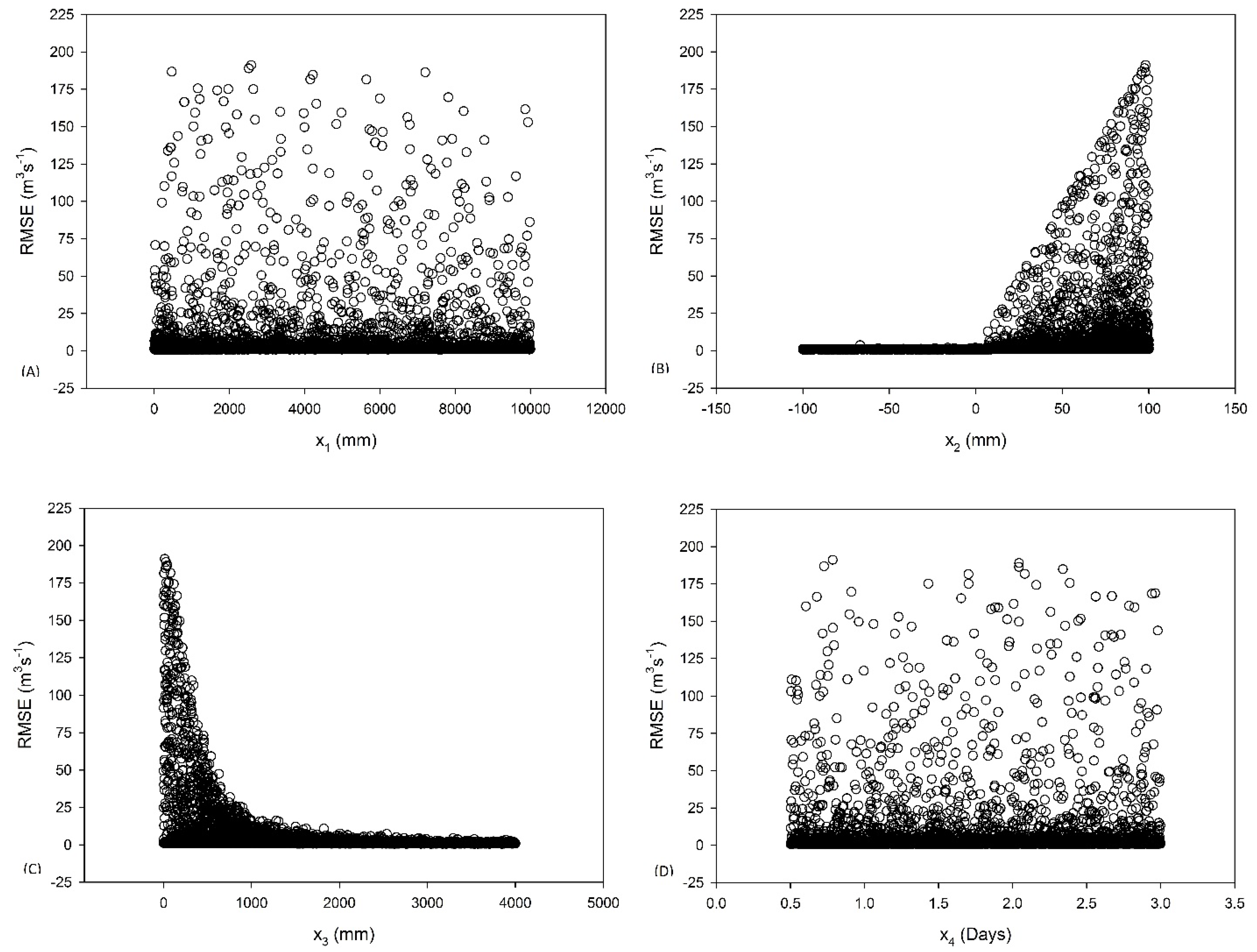
2.7. Sensitivity Analysis

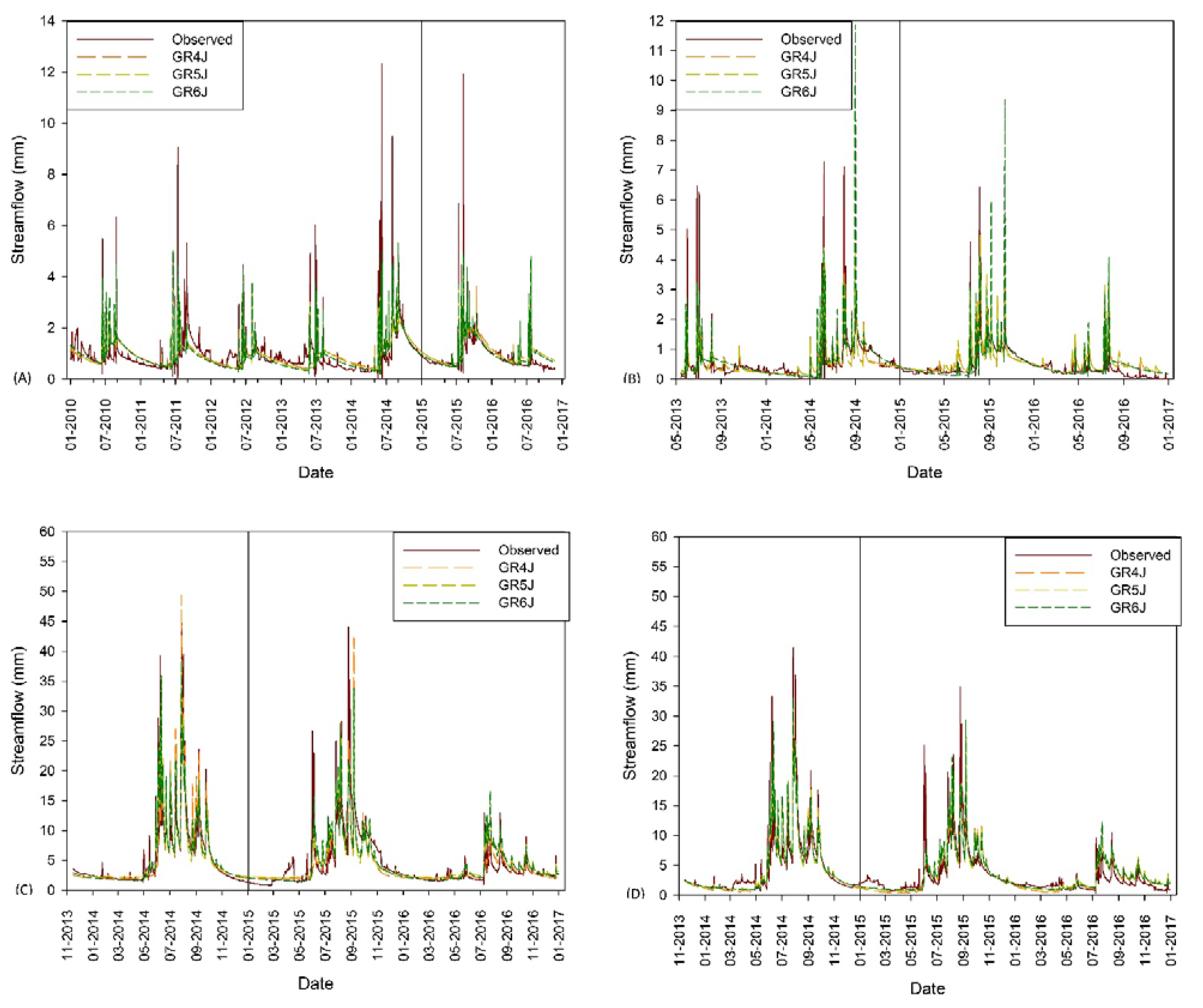
To determine which of the parameters had a greater effect on the quality of the discharge simulation for the GR4J, GR5J and GR6J hydrologic models, the Generalized Probability Uncertainty Estimation (GLUE) sensitivity analysis proposed by [92] was used. This methodology considers as a performance measure the probability that a given set of model parameters will generate satisfactory results regarding the simulation of the behavior of the system under study [92].

A sample size equal to 10,000 random parameter sets was used and the efficiency of each set was determined using the RMSE statistic, which reaches its optimal values as it approaches 0 [85]. Finally, GLUE sensitivity analysis was performed with the Sensitivity Analysis For Everybody (SAFE) toolbox [93,94] in MATLAB software version R2019a [95].

3. Results

3.1. Best Evapotranspiration Model That Maximizes Model Performance

In each of the catchments, we investigated the performance of the GR4J, GR5J and GR6J models using different potential/actual evapotranspiration models. Firstly, we identified the set of parameters that allowed the most efficient simulation in the calibration period according the Mitchell calibration algorithm [75] (

Table 3. Parameter sets that maximize flow simulation efficiency in each basin for GR4J, GR5J and GR6J hydrologic models in calibration period.

		Catchment
Model	Parameter	Q2	Q3	BLQ1	BLQ2
GR4J	X1	109.94	8690.62	979.30	1577.47
	X2	−146.91	−1.62	7.19	2.62
	X3	7500.22	25.79	62.98	197.93
	X4	0.98	1.10	1.41	1.42
GR5J	X1	122.81	10114.94	671.08	1314.74
	X2	−9.21	−1.20	−1.90	0.78
	X3	7598.89	24.74	235.18	212.79
	X4	0.98	0.78	1.15	1.16
	X5	0.13	0.35	1.00	0.00
GR6J	X1	139.10	104.57	323.76	509.16
	X2	−1.18	−2.66	0.52	0.17
	X3	6276.71	2554.09	112.17	123.36
	X4	0.98	1.04	1.48	1.48
	X5	−0.11	−0.03	−0.41	−0.73
	X6	64.39	1.52	96.54	92.45

), those that were obtained from the precipitation and streamflow data, in addition to the evapotranspiration that maximizes the efficiency of the model (

Table 4. Best evapotranspiration models (PET) that maximize hydrological model performance for the calibration period.

		Catchment
		Q2	Q3	BLQ1	BLQ2
GR4J	PET	EO	EO	EH	EO
	KGE	0.569	0.725	0.766	0.81
	KGE’	0.456	0.704	0.813	0.815
	NSE	0.495	0.569	0.72	0.673
	RMSE (mm)	0.525	0.342	2.347	2.016
	IOA	0.84	0.861	0.912	0.904
	MAE (mm)	0.261	0.235	1.182	1.181
	MAPE (%)	34.6	225.1	28.3	43.5
	SI	0.67	0.84	0.49	0.55
	BIAS (mm)	0.073	−0.013	0.39	−0.054
GR5J	PET	EH	EO	EO	EO
	KGE	0.561	0.748	0.753	0.8
	KGE’	0.448	0.721	0.734	0.772
	NSE	0.471	0.553	0.712	0.68
	RMSE (mm)	0.537	0.348	2.38	1.995
	IOA	0.84	0.857	0.905	0.905
	MAE (mm)	0.243	0.234	1.387	1.151
	MAPE (%)	32.5	220.3	37.3	41.8
	SI	0.61	0.89	0.37	0.44
	BIAS (mm)	0.019	−0.028	−0.087	−0.069
GR6J	PET	EPTp	EO	EO	EO
	KGE	0.574	0.818	0.801	0.808
	KGE’	0.471	0.804	0.798	0.781
	NSE	0.395	0.724	0.733	0.683
	RMSE (mm)	0.575	0.273	2.292	1.985
	IOA	0.862	0.824	0.917	0.907
	MAE (mm)	0.229	0.188	1.273	1.093
	MAPE (%)	28.4	192.7	30.4	38
	SI	0.57	0.77	0.37	0.46
	BIAS (mm)	−0.029	−0.0014	−0.0057	0.06

Note: E_H is the Hargreaves–Samani model; E_O is the Oudin model; E_PTp is the potential evapotranspiration according to Priestley–Taylor; E_PTa is the actual evapotranspiration according to Priestley–Taylor.

).

In general, catchment Q2 had lower X₁-X₂-X₄ parameter values and higher X₃ parameter values. The X₅ parameter was in general lower in catchment Q2 and the X₆ parameter was higher in wetter catchments (BLQ1 and 2).

A graphical evaluation of model performance during the calibration and validation periods showed that the three models captured the oscillations inherent to the observed streamflow, so that the simulated values were well harmonized with the observed values (Figure 5).

Potential and actual evapotranspiration models (PET and AET, respectively) tend to have the same trend over time, varying only seasonally in the first summer and autumn–winter months. The highest evapotranspiration values correspond to the E_PTp (Priestley–Taylor), E_PTa (Actual Priestley–Taylor) and E_H (Hargreaves–Samani) methods, which in summer months are on average four and three times higher than Oudin evapotranspiration methods, respectively. On the contrary, the minimum values in summer months are reached by the E_o (Oudin) method. During the winter months, all models achieved similar evapotranspiration values (Figure 6).

The evapotranspiration models that maximized the efficiency of the hydrological models (Table 4) varied according to each model and catchment, with the Oudin evapotranspiration method being the one that maximizes efficiency in most models and catchments. The GR4J model achieved its highest efficiency in catchments Q2, Q3 and BLQ2 using the E_O model, and in BLQ1 with the E_H method. In the GR5J model, the highest efficiency was obtained in catchments Q3, BLQ1 and BLQ2 with the E_O method, and in Q2 with E_H. Finally, the GR6J model reached its highest efficiency in catchments Q3, BLQ1 and BLQ2 when the E_O method was used, and in Q2 when E_PTp was used.

Our results demonstrated that the three hydrological models were capable of efficiently simulating flow in the four study catchments and in general using the Oudin potential evapotranspiration model (Table 4 for calibration period and

Table 5. Efficiency criteria for the validation period in all basins using the GR4J, GR5J and GR6J hydrological models.

		Catchment
		Q2	Q3	BLQ1	BLQ2
GR4J	KGE	0.569	0.725	0.766	0.810
	KGE’	0.456	0.704	0.813	0.815
	NSE	0.495	0.569	0.720	0.673
	RMSE (mm)	0.525	0.342	2.347	2.016
	IOA	0.840	0.861	0.912	0.904
	MAE (mm)	0.261	0.235	1.182	1.181
	MAPE (%)	34.6	225.1	28.3	43.5
	SI	0.59	0.74	0.54	0.65
	BIAS (mm)	0.058	−0.0051	0.058	−0.098
GR5J	KGE	0.561	0.748	0.753	0.800
	KGE’	0.448	0.721	0.734	0.772
	NSE	0.471	0.553	0.712	0.680
	RMSE (mm)	0.537	0.348	2.380	1.995
	IOA	0.840	0.857	0.905	0.905
	MAE (mm)	0.243	0.234	1.387	1.151
	MAPE (%)	32.5	220.3	37.3	41.8
	SI	0.63	0.74	0.58	0.64
	BIAS (mm)	0.026	0.0088	0.18	0.41
GR6J	KGE	0.574	0.818	0.801	0.808
	KGE’	0.471	0.804	0.798	0.781
	NSE	0.395	0.724	0.733	0.683
	RMSE (mm)	0.575	0.273	2.292	1.985
	IOA	0.862	0.824	0.917	0.907
	MAE (mm)	0.229	0.188	1.273	1.093
	MAPE (%)	28.4	192.7	30.4	38.0
	SI	0.54	0.60	0.56	0.64
	BIAS (mm)	0.0061	−0.10	0.12	0.41

for validation) (KGE and KGE’ > 0.45; NSE > 0.3, RMSE < 3.0, IOA > 0.8, MAE < 1.5, MAPE < 45%, SI > 0.37 and −0.10 < BIAS < 0.41). However, the GR6J model obtained the most satisfactory results (Table 4 and Table 5).

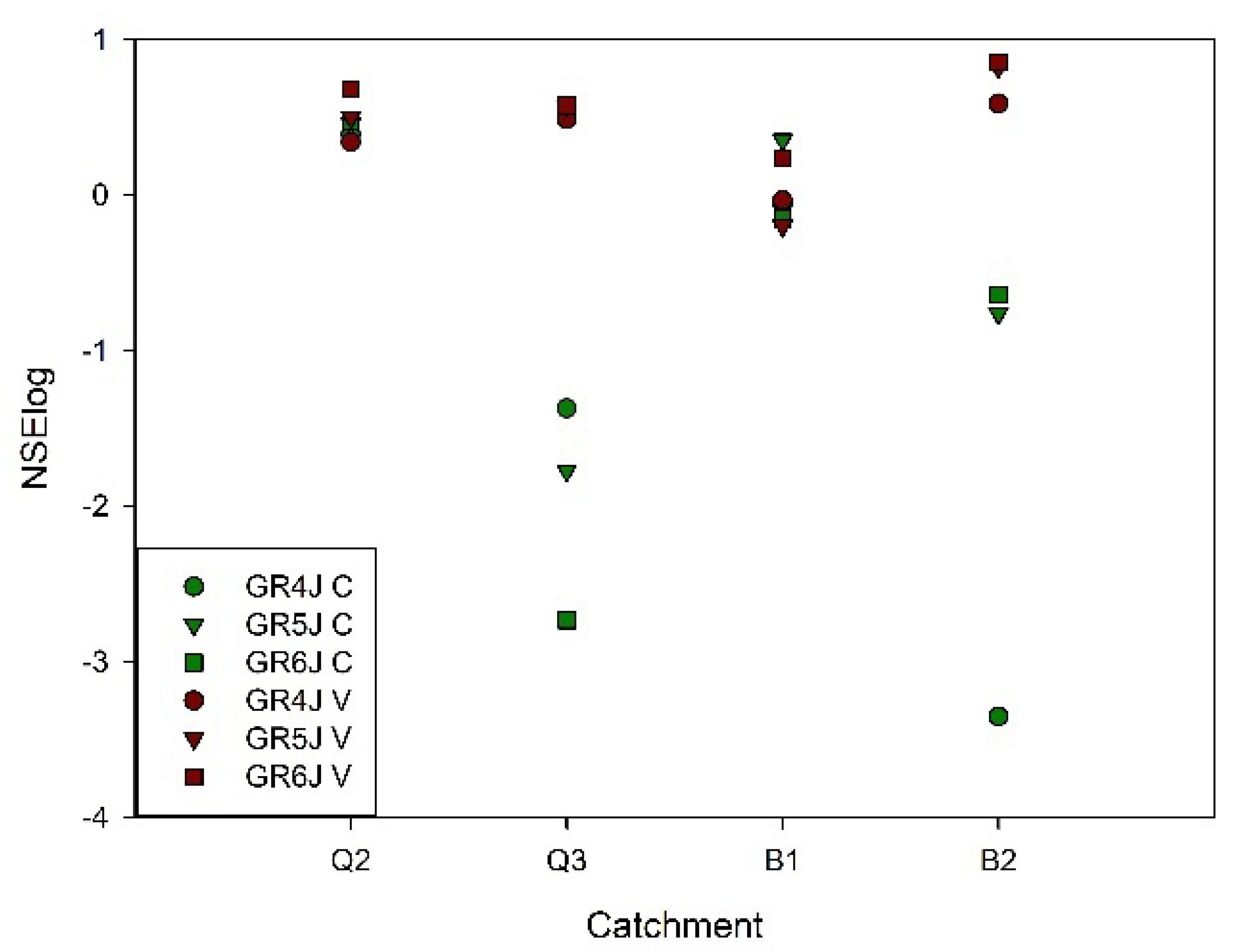
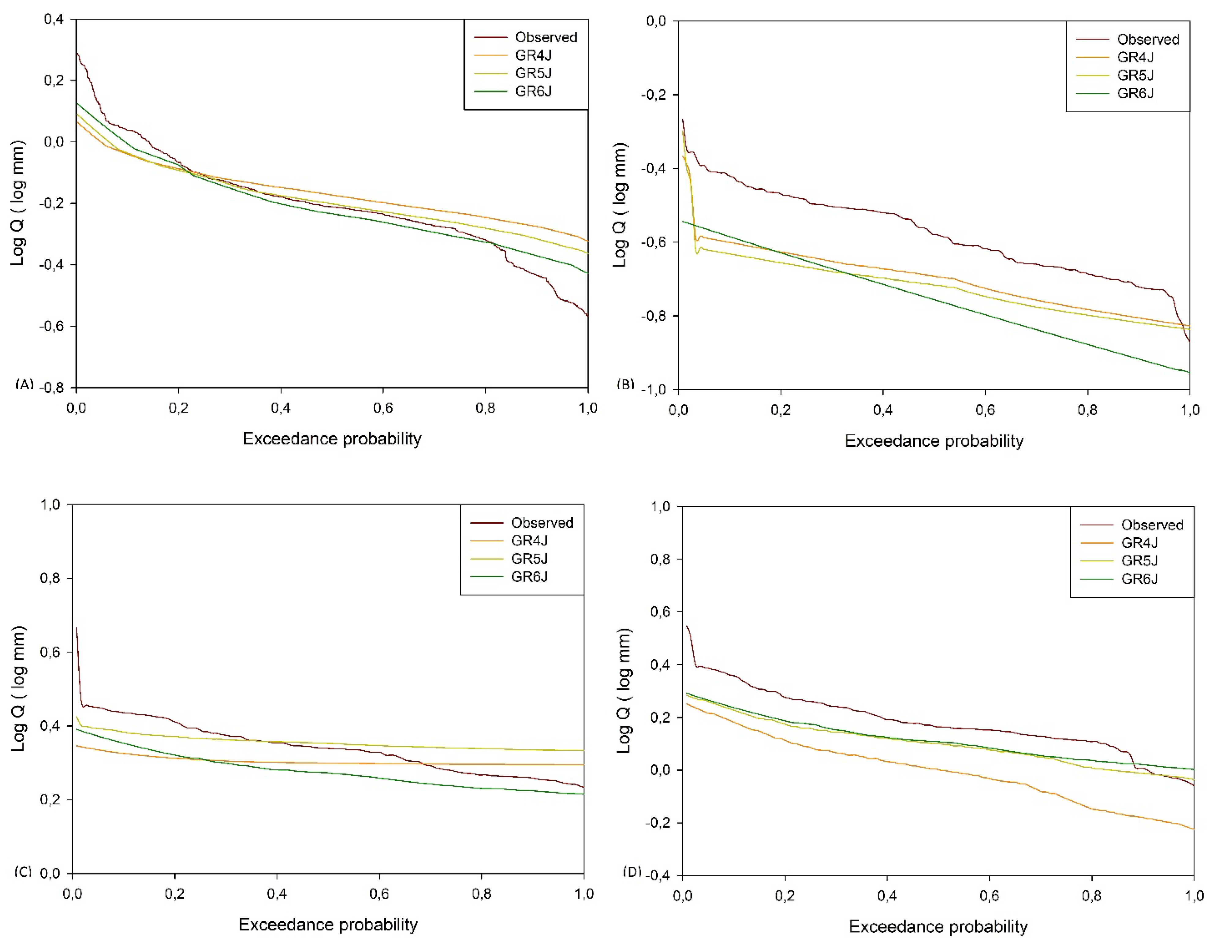
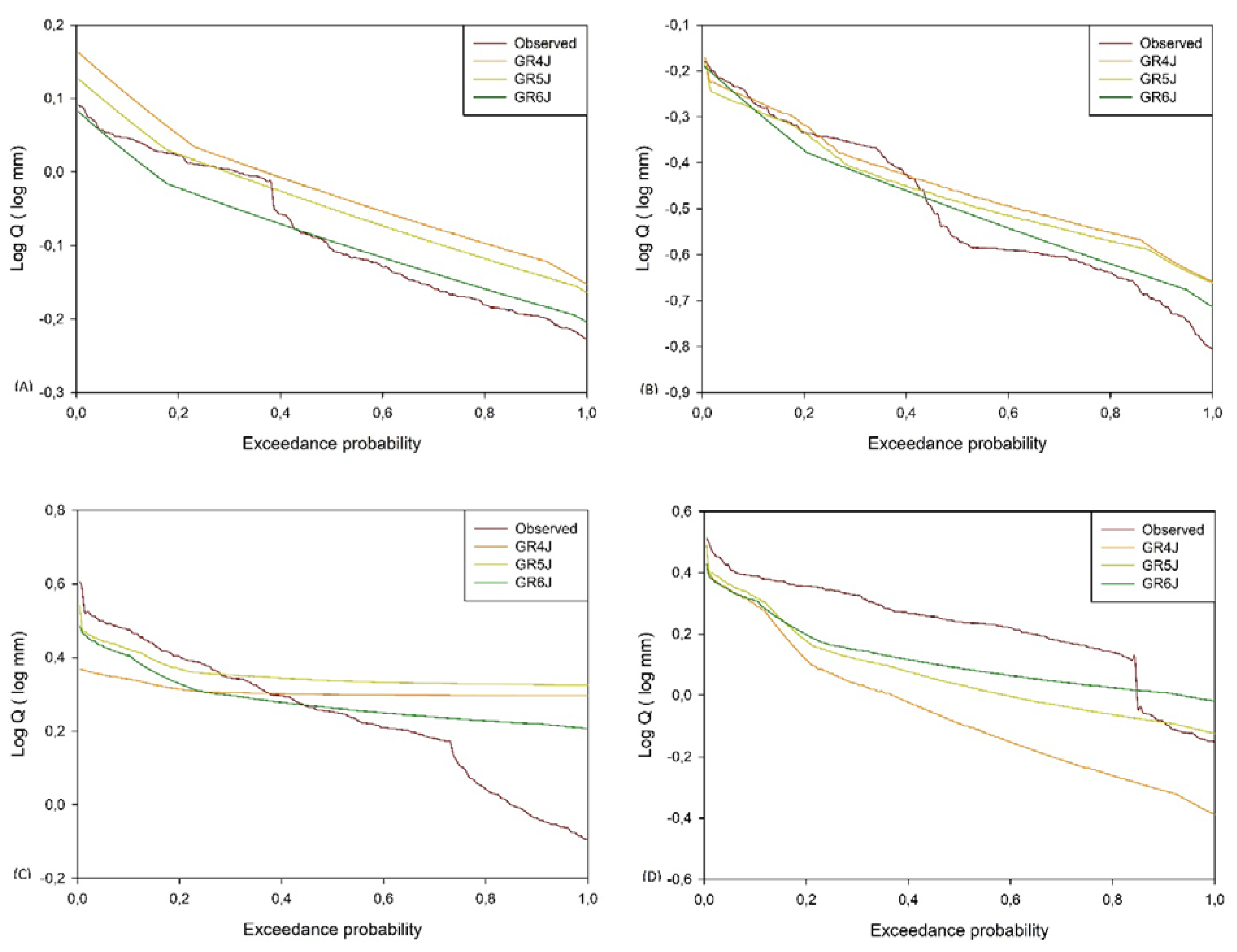
3.2. Peak Flows and Summer Flow

None of the models successfully represent peak flows (Figure 5). For example, in the calibration period of the Q2 catchment (native forest cover), the models showed an underestimation ranging between 20 and 70% for GR4J, 18 and 70% for GR5J and between 10 and 62% for GR6J, while in the validation period the models showed an underestimation ranging between 21 and 62% for GR4J and GR5J and between 15 and 58% for GR6J. In the calibration period of Q3, the models showed an underestimation ranging between 40 and 71% for GR4J, 39 and 72% for GR5J and 43 and 69% for GR6J, while in the validation period the models showed an underestimation ranging between 2 and 35% for GR4J, 6 and 37% for GR5J and between 32 and 35% for GR6J.

Dry season discharge simulation, or summer flow, was not satisfactory in all catchments for all three hydrologic models in the calibration period. NSElog showed low values (<0.5) for all catchments and all models (Figure 7). IOA, MAE, MAPE, SI and BIAS were not used because NSElog estimates better low flows as it decreases the influence of maximum flow rates [91]. However, it was observed that models had low capacity to simulate low flows in detail, but they followed the temporal dynamics of summer flows. The GR6J model had the best performance to simulate low flows; in the same way, all the catchments reached peak values in the validation period rather than in the calibration period.

Additionally, during calibration, the exceedance probability curves showed that GR6J underestimated low flows in Q2, while GR4J and GR5J overestimated low flows lower than 0.8 mm; in Q3 and BLQ2, the three models underestimated low flows; and finally, in BLQ1, GR6J underestimated low flows, while GR4J and GR5J underestimated low flows higher than 2.51 mm and 1.99 mm, respectively. In the validation period, the GR4J and GR5J models overestimated low flows in Q2, while the GR6J model overestimated low flows lower than 0.79 mm; in Q3, the GR4J, GR5J and GR6J models overestimated low flows lower than 0.39 mm, 0.35 mm and 0.34 mm; and in BLQ1, the three models underestimated low flows higher than 1.99 mm for GR4J, 2.2 mm for GR5J and 1.90 mm for GR6J. Finally, GR4J underestimated low flows in BLQ2, while GR5J and GR6J underestimated low flows higher than 0.7 mm and 1.2 mm, respectively (Figure 8 and Figure 9).

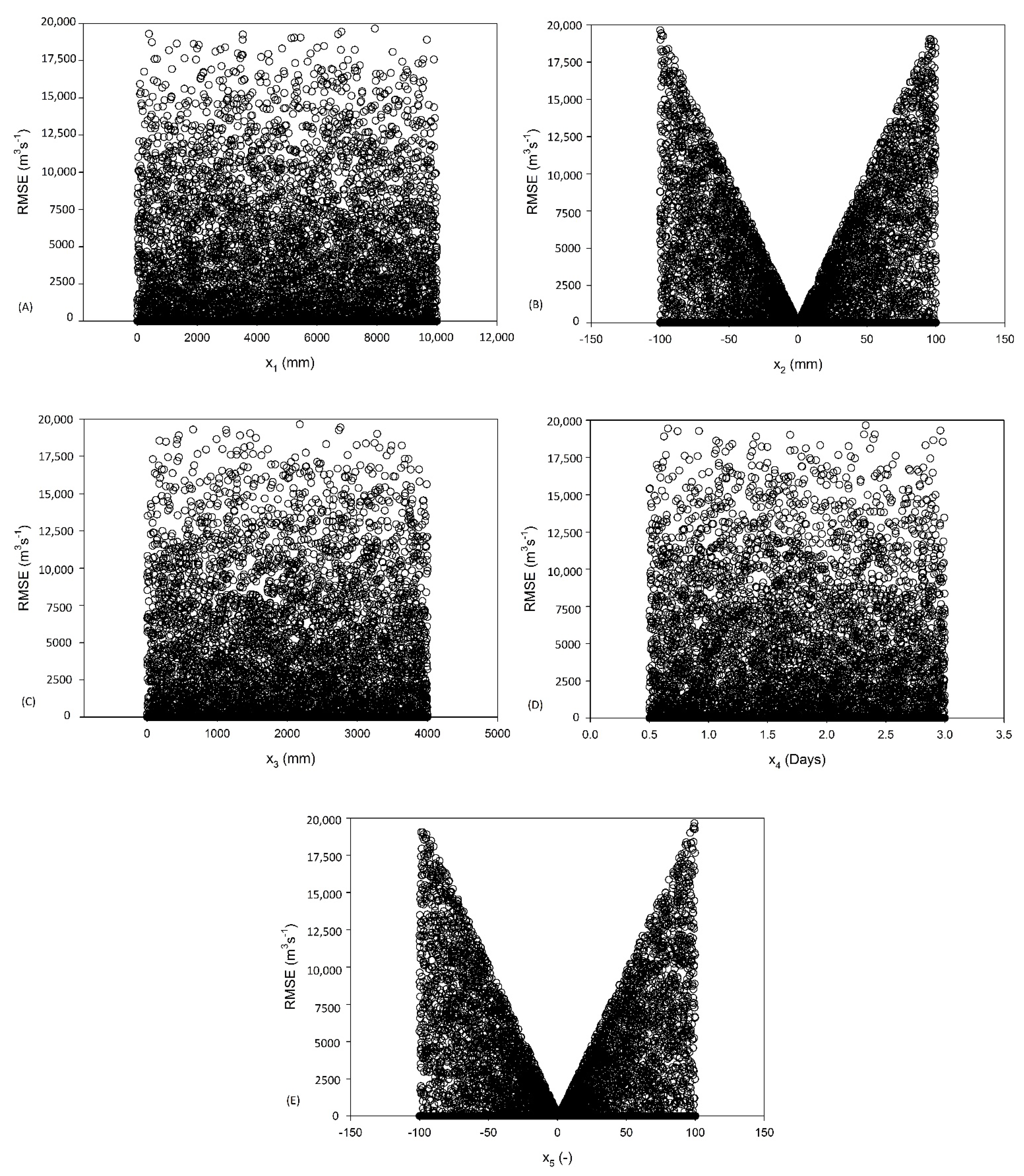
3.3. Sensitivity Analysis

Possible values of the parameters lay in intervals previously identified from the parameters identified in the calibration period for each of the catchments (

Table 6. Low and upper limit of the parameters of the GR4J, GR5J and GR6J hydrological models for the sensitivity analysis.

		GR4J	GR5J	GR6J
X1	Lower limit	0	0	0
	Upper limit	10,000	10,000	10,000
X2	Lower limit	−100	−100	−100
	Upper limit	100	100	100
X3	Lower limit	0	0	0
	Upper limit	4000	4000	4000
X4	Lower limit	0.5	0.5	0.5
	Upper limit	3	3	3
X5	Lower limit	-	−100	−100
	Upper limit	-	100	100
X6	Lower limit	-	-	0
	Upper limit	-	-	500

).

The sensitivity analysis did not show variations between each of the catchments, so catchment Q2 was used to visually represent the results of this analysis. In the GR4J model, parameters X₁ and X₄ showed low sensitivity because a given value of the parameters could be associated with high or low efficiency values. On the contrary, parameters X₂ and X₃ showed high sensitivity since the distribution of the parameter values, and the efficiency statistic RMSE, reflected a clear efficiency trend in both. This means that negative values close to 0 in X₂, and values higher than 2000 in X₃, allowed higher efficiency in the flow simulation (Figure A1 in Appendix A).

In the GR5J and GR6J models, the parameters X₁, X₃ and X₄ showed low sensitivity. In the GR6J model, the parameter X₆ also showed low sensitivity, since a given value of the parameters can be associated with high or low efficiency values. On the contrary, parameters X₂ and X₅ were very sensitive and values close to 0 reached the lowest RMSE values, i.e., higher efficiency. As the parameters moved away from 0, efficiency decreased and RMSE increased (Figure A2 and Figure A3 in Appendix A).

4. Discussion

Our study results showed that the greater complexity of a conceptual hydrological model improves streamflow simulation in small catchments for the hydroclimatic setting (Mediterranean). The results also showed that a complex hydrological model such as GR6J achieved better results in the dry native forest land cover using the Priestley–Taylor potential evapotranspiration model and with Oudin (E_O) in the dry mixed land cover (Q3) and in both wet southern catchments (BLQ1 and BLQ2) with E. nitens land cover. Consistently, Oudin’s potential evapotranspiration model yielded better results in all models and in all catchments. Therefore, our study validated the hypothesis (i) that increasing model complexity will allow for greater efficiency in simulating streamflow in small catchments, and a simpler PET approach also achieved better results, as also showed by Kannan et al. [59] in a small catchment in England and Oudin et al. [48,90].

We accepted the null hypothesis (i) because the GR6J model achieved the most efficient statistics in most of the simulations compared to GR4J and GR5J, which is a similar finding to [96] in Slovenia.

Our hypothesis (ii) that actual evapotranspiration (AET) models can provide better results than potential models (PET) was rejected. PET models achieved more satisfactory results than the actual Priestley–Taylor evapotranspiration model, with PET always being the input data that maximize the efficiency of the models. A plausible explanation for the better performance using PET values is that soil water content limits AET, as E_O yields less ET rates.

4.1. Annual Streamflow

It is important to remember that input data for the hydrological models are PET and not AET. However, this last approach was used to verify the difference in results compared to PET models [22,23,24]. The application of specific evapotranspiration models improved the simulation’s precision in all models.

Our results showed that E_O reaches the lowest value in the evapotranspiration models. However, as pointed out by [97], the Hargreaves–Samani model underestimates the values observed in meteorological stations, while Priestley–Taylor reaches evapotranspiration values that are closer to the observed values.

We observed that Q2 with Q3 and BLQ1 with BLQ2 catchments had similar PET values according to the E_O and E_H model. We also observed that the Priestley–Taylor evapotranspiration model in its potential form (EPTp) yielded similar results in both BLQ1 and 2 paired catchments, with differences around 1.8%. Unlike what is reported by [51] for the GR4J model across the USA, in our study catchments, this model was affected by differences in PET inputs on drier catchments (Q2 and Q3), even though there were water limitations due to lower rainfall and probably less soil water availability.

Consistent to what is reported by [52] in tropical catchments [48,98], all evapotranspiration models predicted streamflow with similar efficiency at all the catchments using the GR4J, GR5J and GR6J models, demonstrating the low sensitivity of the study catchments to changes in PET input values. When using AET, similar efficiencies were achieved to those values obtained when using the different PET models. However, Oudin’s model allowed the highest efficiencies at Q3 and BLQ2 for the three models, in Q2 using the GR4J model and in BLQ1 using the GR5J and GR6J models. These results coincide with those obtained by [48] and confirm that Oudin is the most efficient evapotranspiration method for the hydrological models in our set of catchments and climate.

When GRJ models are combined with evapotranspiration models that overestimate the actual evapotranspiration, a decrease in streamflow simulation quality occurs, especially in low flows and streamflow in dry seasons and dry catchments, while in winter months it is rainfall that mainly induces the streamflow simulation [58]. Thus, if evapotranspiration becomes greater than precipitation (the former artificially overestimated by the model), this would imply that the model does not consider the precipitation input, reducing the lower compartments’ storage. Therefore, it is important to identify the evapotranspiration method that maximizes flow simulation efficiency [22].

Regarding overall model results, our results agreed with studies [99,100], which found that conceptual hydrological models perform better in wetter catchments than drier ones. According to the NSE, IOA, MAE, MAPE and BIAS criteria, the GR6J model was the most efficient in flow simulation, regardless of the temporal extent of the input data. Likewise, a positive correlation was observed between models’ quality and the incoming precipitation (i.e., wet catchments) since simulation efficiency increased for all models in years with higher precipitation records. The NSE, IOA, MAE, MAPE, SI and BIAS criteria were the most sensitive to extreme values in the four study catchments, so they reached suboptimal values when there was a larger number of outliers [101]. However, if the samples are small and the catchments are heterogeneous, as was the case in this study, it is recommended to use the NSE criterion [102]. All RMSE values were low for all catchments (< 2.61). Effectively, this was a useful criterion because it is a good indicator when the simulation is continuous and long-term [103].

4.2. Peak Flows

Regarding peak flows, they were difficult to simulate with the three hydrological models. This is consistent with [104], which showed that peak flows are naturally difficult to model because of the problems of spatial and temporal representation of the most intense precipitation. This is complemented by [105], which showed that the simulation step is another factor that limits the simulation of peak flow events, since not all the catchment area has a homogeneous concentration time [104,106]. Although some attempts have been made to model peak flow, such as [107] that showed good performance on peak flows in east China, the modified model is not able to simulate daily flows. Therefore, our results were expected since this hydrological model family was not specifically designed to model peak flows.

In addition, the RMSE criterion does not seem to be sufficient to describe the ability of the model to simulate peak flows. The streamflow underestimation observed in Q2 is larger than BLQ1 and BLQ2. However, in these last ones, a significantly higher RMSE was obtained due to their higher observed and simulated discharge values. Although our results suggested that the GR6J model achieves better results in simulating maximum flows, these results are contrary to those obtained by [108], where the GR4J model achieves greater peak flow efficiency. More studies are needed to identify the advantages and disadvantages of the GRJ models to simulate peak flows in small catchments.

4.3. Summer Flows

In the lower precipitation period, the Q3 catchment reached a low flow with 0.000013 mm for two months in both the calibration and validation periods, where none of the models were able to simulate them in both periods. However, due to the NSElog criteria and exceedance probability analysis, the GR6J model was the most efficient to simulate low discharge in all study basins.

Our results matched with those obtained by [24,109,110], where the GR6J model achieved a better simulation of minimum flows than the GR4J model, especially in catchments where groundwater contributes significantly to flow. This difference is attributed to the fact that the GR6J model considers a second exponential routing store, the one that is in parallel to the existing routing store in the GR4J and GR5J models associated with an additional parameter (X₆) in the GR6J model. This gave a more accurate simulation of low flows in summer in most of the studied scenarios and does not decrease efficiency in the simulation of maximum flows [24,74]. One possible explanation is that the GR6J exponential routing store is capable of dealing with positive and negative values, so it has the capability to represent water levels even though no water reaches this storage (no precipitation or drainage), and it can therefore simulate the recession stage more efficiently [111].

It should be noted that an uninterrupted series of dry years (2010–2019) has prevailed in central Chile (western South America, 30–38° S), with annual precipitation deficits varying between 25 and 45% [5], during the timespan considered in this study (2010–2016). Therefore, one possible reason for our results is the consequence of the effects of climate change [5]. Low flows in extreme MD and in semi-arid conditions (Q2 and Q3) with mean annual precipitation below 950 mm could be extremely vulnerable to this phenomenon.

It is important to note that, as also pointed out by [51], the variability of the parameters of the same catchment between models, specifically X₂ and X₅ in Q2 and BLQ1, is given by using different evapotranspiration methods. Additionally, the parameters x1, X₂ and X₃ are more sensitive than the parameter x4 to the precipitation input data, while X₃ is more sensitive to the size of the catchment and the length of the water network [112]. For instance, X₁ in BLQ1 changes from 979 to 671 when passing from GR4J to GR5J, while it drops to 323 in GR6J. This means that hydrological processes represented by parameters are re-arranged by the model. Thus, as the variability of the parameter X₁ among the catchments may be related to the variations in the input values of precipitation and not to PET, further analyses are required to accurately identify the sources of variability for parameter X₁.

In the same way, the sensitivity analysis showed that according to the RMSE criterion, parameters X₂ and X₃ in the GR4J model (similar results to those obtained by [113]) and X₂ and X₅ in the GR5J and GR6J models are the most sensitive parameters, explaining its greater variability when using different evapotranspiration input data for the same catchment. So, when a more efficient discharge simulation is needed, they must be calibrated before any other parameters.

From the KGE, KGE’, NSE, RMSE, IOA, MAE, MAPE, SI and BIAS values obtained for the four catchments and their results, it is possible to infer that the random or systematic errors in the input data, such as precipitation, temperature and evapotranspiration, adequately represent the input conditions in time and space throughout the catchment [11].

The robustness of the KGE and KGE’ criteria depend on the climatic variability within each of the catchments, rather than on the objective function that may not be sensitive to the models [114]. This could also be explained by the similar behavior observed in the quality of the simulation between Q2 and Q3 and between BLQ1 and BLQ2 catchments. Here, BLQ2 had a higher quality in the simulation of discharge according to the KGE and KGE’ criteria.

Simulations performed by GR4J, GR5J and GR6J hydrological models were shown to be efficient in reaching the representativeness of the streamflow regime in the study catchments during the calibration and validation periods. In turn, it was observed that the RMSE criteria reached their most efficient values for the Q3 and BLQ1 calibration periods and the Q3, BLQ1 and BLQ2 validation periods when using GR6J.

5. Conclusions

The use of hydrological models has become a valuable tool to analyze water resource management and to better understand the role of the components of the hydrological cycle. Our results highlighted the necessity of selecting the right model to achieve the best results, and to allocate calibration efforts and resources to parameter estimation to improve flow simulation efficiency. For instance, for low flows, a more complex model, such as GR6J, will perform better than a simpler one, such as GR4J.

One of our main results is that conceptual rainfall–runoff models such as GR4J, GR5J and GR6J can be utilized under low data availability areas, but also that no single PET/AET model will work in different climate and catchment land covers. Both potential and actual evapotranspiration models could provide dissimilar results when feeding hydrological models. The use of Oudin, Hargreaves–Samani and Actual Priestley–Taylor models improved the simulation’s performance over the Potential Priestley–Taylor model, which showed no improvement in the efficiency of the hydrological models in any of the study catchments. However, it seems that the Oudin potential evapotranspiration model is better to drive these conceptual models. These results highlight that for modeling small catchments, the use of a temperature-driven PET/AET model is sufficient.

The analyses presented here are limited to this set of data and catchments. As conceptual models are a simplistic representation of several hydrological processes, some processes can be muted or unrepresented. Limitations in physical processes such as soil infiltration and canopy interception can increase streamflow modeling bias. Rainfall and topography are both highly variable, so the exploration of other conceptual lumped models or semi-distributed ones (with low climate input variable requirements) in a wide range of catchments and climates is still necessary.

The higher sensitivity of parameters X₅ and X₆ indicates the importance of below-ground processes such as infiltration, vadose zone storage and groundwater recharge. Additionally, lower ET amounts yield better model performance, which links to plant-related hydrological processes such as root depth, canopy density and orientation. Our results highlight the importance of a better representation of the water movement in the soil–plant–atmosphere continuum. We also note that current soil–water information for the sites does not suffice to improve model efficiency. Detailed simulations of small-scale catchments (less than 1 km²) would also require parameterizing the within-catchment variability of soil–water relationships. Even though variability could be small, it could lead to differences in outputs or switching the prevalence of different hydrological processes. Another limitation lies in the difficulty of giving physical meaning to lumped parameters. Differences in the performance of GRxJ models among catchments also highlight the importance of the hydrological setting.

The within-catchment variability of soil water content could play a key role in actual ET values. The lasting dry condition in central Chile since 2010 could have shifted the ET from forested cover from an energy-limited process to a water-limited one. This issue is also a limitation that requires further analysis.

Our next steps are to further investigate the complexity of other lumped and semi-distributed models and their relationship with the mega-drought. It is also necessary to analyze the impacts of afforestation on water availability due to climate change, and the impact of vegetation cover on the quality of the simulation. Finally, future work on small catchments will include hybrid modeling (lumped hydrological modeling and machine learning) [115] and the use of machine learning techniques [110] to evaluate their efficiency performance in the simulation of maximum and minimum flows.

References

1. Suppan, P.; Kunstmann, H.; Heckl, A.; Rimmer, A. Impact of climate change on wáter availability in. In Climatic Changes and Water Resources in the Middle East and North Africa; Environmental Science and Engineering (Environmental Science); Zereini, F., Hötzl, H., Eds.; Springer: Berlin/Heidelberg, Germany, 2008. [Google Scholar] [CrossRef]
2. Wurbs, R.A.; Muttiah, R.S.; Felden, F. Incorporation of climate change in wáter availability modeling. J. Hydrol. Eng. 2005, 10, 375–385. [Google Scholar] [CrossRef]
3. Balocchi, F.; White, D.A.; Silberstein, R.P.; Ramírez de Arellano, P. Forestal Arauco experimental research catchments; daily rainfall-runoff for 10 catchments with different forest types in Central-Southern Chile. Hydrol. Process. 2021, 35, e14047. [Google Scholar] [CrossRef]
4. Falvey, M.; Garreaud, R.D. Regional cooling in a warming world: Recent temperature trends in the southeast Pacific and along the west coast of subtropical South America (1979–2006). J. Geophys. Res. 2009, 114, D04102. [Google Scholar] [CrossRef]
5. Garreaud, R.D.; Boisier, J.P.; Rondanelli, R.; Montecinos, A.; Sepúlveda, H.H.; Veloso-Aguila, D. The Central Chile mega drought (2010–2018): A climate dynamics perspective. Int. J. Climatol. 2020, 40, 421–439. [Google Scholar] [CrossRef]
6. Muñoz, A.A.; Klock-Barría, K.; Alvarez-Garreton, C.; Aguilera-Betti, I.; González-Reyes, A.; Lastra, J.A.; Chávez, R.O.; Barría, P.; Christie, D.; Rojas-Badilla, M.; et al. Water crisis in Petorca Basin, Chile: The combined effects of a mega-drought and water management. Water 2020, 12, 648. [Google Scholar] [CrossRef] [Green Version]
7. Sarricolea, P.; Serrano-Notivoli, R.; Fuentealba, M.; Hernández-Mora, M.; de la Barrera, F.; Smith, P.; Meseguer-Ruiz, O. Recent wildfires in Central Chile: Detecting links between burned areas and population exposure in the wildland urban interface. Sci. Total Environ. 2020, 706, 135894. [Google Scholar] [CrossRef]
8. Devia, G.K.; Ganasri, B.P.; Dwarakish, G.S. Review on hydrological models. Aquat. Procedian 2015, 4, 1001–1007. [Google Scholar] [CrossRef]
9. Kratzert, F.; Klotz, D.; Brenner, C.; Schulz, K.; Herrnegger, M. Rainfall-runoff modelling using Long Short-Term Memory (LSTM) networks. Hydrol. Earth Syst. Sci. 2018, 22, 6005–6022. [Google Scholar] [CrossRef] [Green Version]
10. Wagener, T.; Boyle, D.P.; Lees, M.J.; Wheater, H.S.; Gupta, H.V.; Sorooshian, S. A framework for development and application of hydrological models. Hydrol. Earth Syst. Sci. 2001, 5, 13–26. [Google Scholar] [CrossRef]
11. Abbott, M.; Refsgaard, J. Distributed Hydrological Modelling; Kluwer Academic Publishers: Dordrecht, The Netherlands, 1996. [Google Scholar] [CrossRef]
12. Hamilton, L. Forest and Water. In FAO Forestry Paper 155; Food and Agriculture Organization of the United Nations: Rome, Italy, 2008; Volume 93, p. 7. [Google Scholar]
13. Yu, Z. Hydrology, floods and droughts. Encycl. Atmos. Sci. 2015, 217–223. [Google Scholar] [CrossRef]
14. Madsen, H. Automatic calibration of a conceptual rainfall–runoff model using multiple objectives. J. Hydrol. 2000, 235, 276–288. [Google Scholar] [CrossRef]
15. Mahe, G.; Paturel, J.E.; Servat, E.; Conway, D.; Dezetter, A. The impact of land use change on soil water holding capacity and river flow modelling in the Nakambe River, Burkina-Faso. J. Hydrol. 2005, 300, 33–43. [Google Scholar] [CrossRef]
16. Muzik, I. A first-order analysis of the climate change effect on flood frequencies in a subalpine catchment by means of a hydrological rainfall–runoff model. J. Hydrol. 2002, 267, 65–73. [Google Scholar] [CrossRef]
17. Jukić, D.; Denić-Jukić, V. Groundwater balance estimation in karst by using a conceptual rainfall–runoff model. J. Hydrol. 2009, 373, 302–315. [Google Scholar] [CrossRef]
18. Liu, Y.; Bralts, V.F.; Engel, B.A. Evaluating the effectiveness of management practices on hydrology and water quality at catchment scale with a rainfall-runoff model. Sci. Total. Environ. 2015, 511, 298–308. [Google Scholar] [CrossRef] [PubMed]
19. Beven, K.J. A discussion of distributed hydrological modelling. Water Sci. Technol. Libr. 1990, 22, 255–278. [Google Scholar] [CrossRef]
20. Dutta, P.; Sarma, A.K. Hydrological modeling as a tool for water resources management of the data-scarce Brahmaputra basin. J. Water Clim. Chang. 2021, 12, 152–165. [Google Scholar] [CrossRef] [Green Version]
21. Kumari, N.; Srivastava, A.; Sahoo, B.; Raghuwanshi, N.S.; Bretreger, D. Identification of Suitable Hydrological Models for Streamflow Assessment in the Kangsabati River Basin, India, by Using Different Model Selection Scores. Nat. Resour. Res. 2021, 30, 4187–4205. [Google Scholar] [CrossRef]
22. Perrin, C.; Michel, C.; Andréassian, V. Improvement of a parsimonious model for streamflow simulation. J. Hydrol. 2003, 279, 275–289. [Google Scholar] [CrossRef]
23. Le Moine, N. Le Bassin Versant de Surface Vu par le Souterrain: Une Voie D’amélioration des Performances et du Realisme des Modèles Pluie-Débit? Ph.D. Thesis, Université Pierre et Marie Curie Paris VI, Paris, France, 2008. Available online: https://hal.inrae.fr/tel-02591478 (accessed on 10 August 2021).
24. Pushpalatha, R.; Perrin, C.; Le Moine, N.; Andréassian, V. A downward structural sensitivity analysis of hydrological models to improve low-flow simulation. J. Hydrol. 2011, 411, 66–76. [Google Scholar] [CrossRef]
25. Boyle, D.P.; Gupta, H.V.; Sorooshian, S. Toward improved calibration of hydrologic models: Combining the strengths of manual and automatic methods. Water Resour. Res. 2000, 36, 3663–3674. [Google Scholar] [CrossRef]
26. Bergström, S. The HBV model. In Computer Models of Watershed Hydrology; Singh, V.P., Ed.; Water Resources Publications: Highlands Ranch, CO, USA, 1995; pp. 443–476. [Google Scholar]
27. Martina, M.L.V.; Todini, E.; Liu, Z. Preserving the dominant physical processes in a lumped hydrological model. J. Hydrol. 2011, 399, 121–131. [Google Scholar] [CrossRef]
28. Cornelissen, T.; Diekkrüger, B.; Giertz, S. A comparison of hydrological models for assessing the impact of land use and climate change on discharge in a tropical catchment. J. Hydrol. 2013, 498, 221–236. [Google Scholar] [CrossRef]
29. Givati, A.; Thirel, G.; Rosenfeld, D.; Paz, D. Climate change impacts on streamflow at the upper Jordan River based on an ensemble of regional climate models. J. Hydrol. Reg. Stud. 2019, 21, 92–109. [Google Scholar] [CrossRef]
30. Boumenni, H.; Bachnou, A.; Alaa, N.E. The rainfall-runoff model GR4J optimization of parameters by genetic algorithms and Gauss-Newton method: Application for the watershed Ourika (High Atlas, Morocco). Arab. J. Geosci. 2017, 10, 343. [Google Scholar] [CrossRef]
31. Dao, A.; Fadika, V.; Noufe, D.D.; Diaby, A.A.; Kamagate, B. Contribution of GR6J model to the assessment of the water balance for theBETE sub-basin (Aghienlagoon, southern Côte d’Ivoire). EWASH TI J. 2019, 3, 104–112. [Google Scholar]
32. Delpasand, R.; Fathabadi, A.; Rouhani, H.; Seyedian, S.M. Evaluating the Efficiency of K nearest Neighbor and Fuzzy C-Means Clustering Based Methods in the Outputs of Hydrological Models. Water Manag. Res. 2019, 32, 63–77. [Google Scholar]
33. Kunnat-Poovakka, A.; Eldho, T.I. A comparative study of conceptual rainfall-runoff models GR4J, AWBM and Sacramento at catchments in the upper Godavari River basin, India. J. Earth Syst. Sci. 2019, 128, 33. [Google Scholar] [CrossRef] [Green Version]
34. Lujano, E.; Sosa, J.D.; Lujano, R.; Lujano, A. Performance evaluation of hydrological models GR4J, HBV and SOCONT for the forecast of average daily flows in the Ramis River basin, Perú. Rev. Ing. UC 2020, 27, 189–199. [Google Scholar]
35. Barría, P.; Barría, I.; Guzman, C.; Chadwik, C.; Alvarez-Garreton, C.; Ocampo-Melgar, A.; Fuster, R. Water allocation under climate change: A diagnosis of the Chilean system. Elem. Sci. Anthr. 2021, 9, 00131. [Google Scholar] [CrossRef]
36. Muñoz-Castro, E.; Mendoza, P.; Vargas, X. The role of parameter estimation strategies on ensemble streamflow prediction results across extratropical Andean catchments. In EGU General Assembly 2020; EGU2020-10845; Copernicus Publications: Munich, Germany, 2020. [Google Scholar] [CrossRef]
37. Ruelland, D.; Dezetter, A.; Hublart, P. Sensitivity analysis of hydrological modelling to climate forcing in a semi-arid mountainous catchment. In Proceedings of the FRIEND-Water 2014, Montpellier, France, 7–10 October 2014. [Google Scholar]
38. Hublart, P.; Ruelland, D.; García de Cortázar Atauri, I.; Ibacache, A. Reliability of a conceptual hydrological model in a semi-arid Andean catchment facing water-use changes. Proc. Int. Assoc. Hydrol. Sci. 2015, 371, 203–209. [Google Scholar] [CrossRef] [Green Version]
39. Sood, A.; Smakhtin, V. Global hydrological models: A review. Hydrol. Sci. J. 2015, 60, 549–565. [Google Scholar] [CrossRef]
40. Borges Ferreira, L.; França de Cunha, F.; Alves de Oliveira, R.; Fernandes Filho, E.I. Estimation of reference Evapotranspiration in Brazil with limited meteorological data using ANN and SVM-A new approach. J. Hydrol. 2019, 572, 556–570. [Google Scholar] [CrossRef]
41. Bormann, H.; Diekkrüger, B.; Richter, O. Effects of data availability on estimation of evapotranspiration. Phys. Chem. Earth 1996, 21, 171–175. [Google Scholar] [CrossRef]
42. Dezsi, S.; Mîndrescu, M.; Petrea, D.; Kumar Rai, P.; Hamann, A.; Nistor, M. High-resolution projections of evapotranspiration and water availability for Europe under climate change. Int. J. Climatol. 2018, 38, 3832–3841. [Google Scholar] [CrossRef]
43. Srivastava, A.; Sahoo, B.; Singh Raghuwanshi, N.; Singh, R. Evaluation of Variable-Infiltration Capacity Model and MODIS-Terra Satellite-Derived Grid-Scale Evapotranspiration Estimates in a River Basin with Tropical Monsoon-Type Climatology. J. Irrig. Drain. Eng. 2017, 143, 04017028. [Google Scholar] [CrossRef] [Green Version]
44. Elbeltagi, A.; Kumari, N.; Dharpure, J.K.; Mokhtar, A.; Alsafadi, K.; Kumar, M.; Mehdinejadiani, B.; Etedali, H.R.; Brouziyne, Y.; Reza, M.; et al. Prediction of Combined Terrestrial Evapotranspiration Index (CTEI) over Large River Basin Based on Machine Learning Approaches. Water 2021, 13, 547. [Google Scholar] [CrossRef]
45. Adamala, S.; Raghuwanshi, N.S.; Mishra, A.; Tiwari, M.K. Evapotranspiration Modeling Using Second-Order Neural Networks. J. Hydrol. Eng. 2014, 19, 1131–1140. [Google Scholar] [CrossRef]
46. Talsma, C.; Good, S.P.; Jimenez, C.; Martens, B.; Fisher, J.B.; Miralles, D.G.; McCabe, M.F.; Purdy, A.J. Partitioning of evapotranspiration in remote sensing-based models. Agric. For. Meteorol. 2018, 260–261, 131–143. [Google Scholar] [CrossRef]
47. Hellwig, J.; Stahl, K.; Ziese, M.; Becker, A. The impact of the resolution of meteorological data sets on catchment-scale precipitation and drought studies. Int. J. Climatol. 2018, 38, 3069–3081. [Google Scholar] [CrossRef]
48. Oudin, L.; Hervieu, F.; Michel, C.; Perrin, C.; Andréassian, V.; Anctil, F.; Loumagne, C. Which potential evapotranspiration input for a lumped rainfall–runoff model? Part 2—Towards a simple and efficient potential evapotranspiration model for rainfall–runoff modelling. J. Hydrol. 2005, 303, 290–306. [Google Scholar] [CrossRef]
49. McColl, K.A. Practical and theoretical benefits of an alternative to the Penman-Monteith evapotranspiration equation. Water Resour. Res. 2020, 56. [Google Scholar] [CrossRef]
50. Liu, C.; Sun, G.; McNulty, S.G.; Noormets, A.; Fang, Y. Environmental controls on seasonal ecosystem evapotranspiration/potential evapotranspiration ratio as determined by the global eddy flux measurements. Hydrol. Earth Syst. Sci. 2017, 21, 311–322. [Google Scholar] [CrossRef] [Green Version]
51. Jayathilake, D.I.; Smith, T. Assessing the impact of PET estimation methods on hydrologic model performance. Hydrol. Res. 2021, 52, 373–388. [Google Scholar] [CrossRef]
52. Kodja, D.J.; Sègla Akognongbé, A.J.; Amoussou, E.; Mahé, G.; Vissin1, E.W.; Paturel, J.-E.; Houndénou, C. Calibration of the hydrological model GR4J from potential evapotranspiration estimates by the Penman-Monteith and Oudin methods in the Ouémé watershed (West Africa). Proc. IAHS 2020, 383, 163–169. [Google Scholar] [CrossRef]
53. Guo, D.; Westra, S.; Maier, H.R. Impact of evapotranspiration process representation on runoff projections from conceptual rainfall-runoff models. Water Resour. Res. 2017, 53, 435–454. [Google Scholar] [CrossRef]
54. Alvarez-Garreton, C.; Mendoza, P.A.; Boisier, J.P.; Addor, N.; Galleguillos, M.; Zambrano-Bigiarini, M.; Lara, A.; Puelma, C.; Cortes, G.; Garreaud, R.; et al. The CAMELS-CL dataset: Catchment attributes and meteorology for large sample studies—Chile dataset. Hydrol. Earth Syst. Sci. 2018, 22, 5817–5846. [Google Scholar] [CrossRef] [Green Version]
55. Priestley, C.; Taylor, R. On the assessment of surface heat flux and evaporation using large-scale parameters. Mon. Weather Rev. 1972, 100, 81–92. [Google Scholar] [CrossRef]
56. van Heerwaarden, C.C.; Vilà-Guerau de Arellano, J.; Teuling, A.J. Land-atmosphere coupling explains the link between pan evaporation and actual evapotranspiration trends in a changing climate. Geophys. Res. Lett. 2010, 37, L21401. [Google Scholar] [CrossRef] [Green Version]
57. Zhao, L.; Xia, J.; Xu, C.; Wang, Z.; Sobkowiak, L.; Long, C. Evapotranspiration estimation methods in hydrological models. J. Geogr. Sci. 2013, 23, 359–369. [Google Scholar] [CrossRef]
58. Aouissi, J.; Benabdallah, S.; Chabaâne, Z.L.; Cudennec, C. Evaluation of potential Evapotranspiration assessment methods for hydrological modelling with SWAT-Application in data-scarce rural Tunisia. Agric. Water Manag. 2016, 174, 39–51. [Google Scholar] [CrossRef]
59. Kannan, N.; White, S.M.; Worral, F.; Whelan, M.J. Sensitivity analysis and identification of the best evapotranspiration and runoff options for hydrological modelling in SWAT-2000. J. Hydrol. 2007, 332, 456–466. [Google Scholar] [CrossRef]
60. Martínez-Retureta, R.; Aguayo, M.; Stehr, A.; Sauvage, S.; Echeverría, C.; Sánchez-Pérez, J.M. Effect of Land Use/Cover Change on the Hydrological Response of a Southern Center Basin of Chile. Water 2020, 12, 302. [Google Scholar] [CrossRef] [Green Version]
61. Iroumé, A.; Jones, J.; Bathurst, J.C. Forest operations, tree species composition and decline in rainfall explain runoff changes in the Nacimiento experimental catchments, south central Chile. Hydrol. Process. 2021, 35, e14257. [Google Scholar] [CrossRef]
62. McNamara, I.; Nauditt, A.; Zambrano-Bigiarini, M.; Ribbe, L.; Hann, H. Modelling water resources for planning irrigation development in drought-prone southern chile. Int. J. Water Resour. Dev. 2020, 1–26. [Google Scholar] [CrossRef]
63. Smith, M.B.; Koren, V.; Reed, S.; Zhang, Z.; Zhang, Y.; Moreda, F.; Cui, Z.; Mizukami, N.; Anderson, E.A.; Cosgrove, B.A. The distributed model intercomparison project–Phase 2: Motivation and design of the Oklahoma experiments. J. Hydrol. 2012, 418, 3–16. [Google Scholar] [CrossRef] [Green Version]
64. Velázquez, J.A.; Troin, M.; Caya, D. Hydrological modeling of the Tampaon River in the context of climate change. Tecnol. Cienc. Agua 2015, 6, 17–30. Available online: http://revistatyca.org.mx/ojs/index.php/tyca/article/view/1167 (accessed on 10 August 2021).
65. Anshuman, A.; Kunnath-Poovakka, A.; Eldho, T.I. Performance evaluation of conceptual rainfall-runoff models GR4J and AWBM. ISH J. Hydraul. Eng. 2018, 27, 365–374. [Google Scholar] [CrossRef]
66. Brulebois, E.; Ubertosi, M.; Castel, T.; Richard, Y.; Sauvage, S.; Perez, J.M.; Le Moine, N.; Amiotte-Suchet, P. Robutness and performance of semi-distributed (SWAT) and global (GR4J) hydrological models throughout an observed climatic shift over contrasted French catchments. Open Water J. 2018, 5, 41–56. [Google Scholar]
67. Gan, Y.; Duan, Q.; Gong, W.; Tong, C.; Sun, Y.; Chu, W.; Ye, A.; Miao, C.; Di, Z. A comprehensive evaluation of various sensitivity analysis methods: A casa study with a hydrological model. Environ. Model. Softw. 2014, 51, 269–285. [Google Scholar] [CrossRef] [Green Version]
68. Balocchi, F.; Flores, N.; Neary, D.; White, D.A.; Silbrestein, R.P.; Ramírez de Arellano, P. The effect of the ‘Las Maquinas’ wildfire of 2017 on the hydrologic balance of a high conservation value Hualo (Nothofagus glauca (Phil.) Krasser) forest in central Chile. For. Ecol. Manag. 2020, 477, 118482. [Google Scholar] [CrossRef]
69. Stolpe, N. Descripciones de los principales suelos de la VIII Región de Chile. In Publicaciones del Departamento de Suelos y Recursos Naturales; Facultad de Agronomía, Universidad de Concepción: Concepción, Chile, 2006; p. 83. [Google Scholar]
70. Coops, N.C.; Waring, R.H.; Moncrieff, J.B. Estimating mean monthly incident solar radiation on horizontal and inclined slopes from mean monthly temperatures extremes. Int. J. Biometeorol. 2000, 44, 204–211. [Google Scholar] [CrossRef]
71. Sezen, C.; Bezak, N.; Šraj, M. Hydrological modelling of the karst Ljubljanica River catchment using lumped conceptual model. Acta Hydrotech. 2018, 31, 87–100. [Google Scholar] [CrossRef]
72. Sezen, C.; Bezak, N.; Bai, Y.; Šraj, M. Hydrological modelling of karst catchment using lumped conceptual and data mining models. J. Hydrol. 2019, 576, 98–110. [Google Scholar] [CrossRef]
73. Carvajal, L.F.; Roldán, E. Calibración del modelo lluvia-escorrentía agregado GR4J aplicación: Cuenca del río aburrá. Dyna 2007, 74, 73–87. Available online: https://revistas.unal.edu.co/index.php/dyna/article/view/912 (accessed on 10 August 2021).
74. Coron, L.; Thirel, G.; Delaigue, O.; Perrin, C.; Andréassian, V. The suite of lumped GR hydrological models in an R package. Environ. Model. Softw. 2017, 94, 166–171. [Google Scholar] [CrossRef]
75. Coron, L.; Delaigue, O.; Thirel, G.; Perrin, C.; Michel, C.; Andréassian, V.; Bourgin, F.; Brigode, P.; Le Moine, N.; Mathevet, T.; et al. airGR: Suite of GR Hydrological Models for Precipitation-Runoff Modelling; R Package Version 1.6.12; Available online: https://CRAN.R-project.org/package=airGR (accessed on 10 August 2021). [CrossRef]
76. Hargreaves, G.H.; Samani, Z.A. Estimating potential evapotranspiration. J. Irrig. Drain. Div. 1982, 108, 225–230. [Google Scholar] [CrossRef]
77. Lhomme, J. A theoretical basis for the Priestley-Taylor coefficient. Bound.-Layer Meteorol. 1997, 82, 179–191. [Google Scholar] [CrossRef]
78. Engstrom, R.; Hope, A.; Kwon, H.; Harazono, Y.; Mano, M.; Oechel, W. Modeling evapotranspiration in Arctic coastal plain ecosystems using a modified BIOME-BGC model. J. Geophys. Res. Biogeosci. 2006, 111. [Google Scholar] [CrossRef]
79. Gan, Y.; Liu, Y.; Pan, X.; Zhao, X.; Li, M.; Wang, S. Seasonal and diurnal variations in the Priestley-Taylor coefficient for a large ephemeral lake. Water 2020, 12, 849. [Google Scholar] [CrossRef] [Green Version]
80. Komatsu, H. Forest categorization according to dry-canopy evaporation rates in the growing season: Comparison of the Priestley–Taylor coefficient values from various observation sites. Hydrol. Process. Int. J. 2005, 19, 3873–3896. [Google Scholar] [CrossRef]
81. Liu, X.; Sun, G.; Mitra, B.; Noormets, A.; Gavazzi, M.J.; Domec, J.C.; Hallema, D.W.; Li, J.; Fang, Y.; King, J.S.; et al. Drought and thinning have limited impacts on evapotranspiration in a managed pine plantation on the southeastern United States coastal plain. Agric. For. Meteorol. 2018, 262, 14–23. [Google Scholar] [CrossRef]
82. Traore, V.; Sambou, S.; Tamba, S.; Fall, S.; Diaw, A.T.; Cisse, M.T. Calibrating the rainfall-runoff model GR4J on the Koulountou river basin, a tributary of the Gambia river. Am. J. Environ. Protect. 2014, 3, 36–44. [Google Scholar] [CrossRef] [Green Version]
83. Piechota, T.C.; Chiew, F.H.S.; Dracup, J.A.; McMahon, T.A. Development of Exceedance Probability Streamflow Forecast. J. Hydrol. Eng. 2001, 6, 20–28. [Google Scholar] [CrossRef]
84. Gupta, H.V.; Kling, H.; Yilmaz, K.K.; Martinez, G.F. Decomposition of the mean squared error and NSE performance criteria: Implications for improving hydrological modelling. J. Hydrol. 2009, 377, 80–91. [Google Scholar] [CrossRef] [Green Version]
85. Nash, J.E.; Sutcliffe, J.V. River flow forecasting through conceptual models part I—A discussion of principles. J. Hydrol. 1970, 10, 282–290. [Google Scholar] [CrossRef]
86. Najafzadeh, M.; Homaei, F.; Farhadi, H. Reliability assessment of water quality index based on guidelines of national sanitation foundation in natural streams: Integration of remote sensing and data-driven models. Artif. Intell. Rev. 2021, 54, 4619–4651. [Google Scholar] [CrossRef]
87. Najafzadeh, M. Evaluation of conjugate depths of hydraulic jump in circular pipe using evolutionary computing. Methodol. Appl. 2019, 23, 13375–13391. [Google Scholar] [CrossRef]
88. Najafzadeh, M.; Oliveto, G. More reliable predictions of clear-water scour depth at pile groups by robust artificial inteligente techniques while preserving physical consistency. Soft Comput. 2021, 25, 5723–5746. [Google Scholar] [CrossRef]
89. Costa do Santos, C.A.; Barbosa da Silva, B.; Ramana, T.V.; Satyamurty, P.; Manzi, A.O. Downward longwave radiation estimates for clear-sky conditions over northeast Brazil. Bras. Meteorol. 2011, 26, 443–450. [Google Scholar] [CrossRef] [Green Version]
90. Oudin, L.; Andréassian, V.; Mathevet, T.; Perrin, C.; Michel, C. Dynamic averaging of rainfall-runoff model simulations from complementary model parameterizations. Water Resour. Res. 2006, 42. [Google Scholar] [CrossRef]
91. Krause, P.; Boyle, D.P.; Bäse, F. Comparison of different efficiency criteria for hydrological model assessment. Adv. Geosci. 2005, 5, 89–97. [Google Scholar] [CrossRef] [Green Version]
92. Beven, K.; Binley, A. The future of distributed models: Model calibration and uncertainty prediction. Hydrol. Process. 1992, 6, 279–298. [Google Scholar] [CrossRef]
93. Pianosi, F.; Sarrazin, F.; Wagener, T. A Matlab toolbox for Global Sensitivity Analysis. Environ. Model. Softw. 2015, 70, 80–85. [Google Scholar] [CrossRef] [Green Version]
94. Pianosi, F.; Beven, K.; Freer, J.; Hall, J.W.; Rougier, J.; Stephenson, D.B.; Wagener, T. Sensitivity analysis of environmental models: A systematic review with practical workflow. Environ. Model. Softw. 2016, 79, 214–232. [Google Scholar] [CrossRef]
95. MATLAB. Version 7.10.0 (R2010a); The MathWorks Inc.: Natick, MA, USA, 2010. [Google Scholar]
96. Lavtar, K.; Bezak, N.; Šraj, M. Rainfall-runoff modeling of the nested non-homogeneous Sava River sub-catchments in Slovenia. Water 2020, 12, 128. [Google Scholar] [CrossRef] [Green Version]
97. Boccheti, M.J.; Muñoz, E.; Tume, P.; Bech, J. Analysis of three indirect methods for estimating the evapotranspiration in the agricultural zone of Chillán, Chile. Obras Proy. 2018, 19, 74–81. [Google Scholar] [CrossRef]
98. Andréassian, V.; Perrin, C.; Michel, C. Impact of imperfect potential evapotranspiration knowledge on the efficiency and parameters of watershed models. J. Hydrol. 2004, 286, 19–35. [Google Scholar] [CrossRef]
99. Van Esse, W.R.; Perrin, C.; Booij, M.J.; Augustijn, D.C.M.; Fenecia, F.; Kavetski, D.; Lobligeois, F. The influence of conceptual model structure on model performance: A comparative study for 237 French catchments. Hydrol. Earth Syst. Sci. 2013, 17, 4227–4239. [Google Scholar] [CrossRef] [Green Version]
100. Merz, R.; Parajka, J.; Blöschl, G. Scale effects in conceptual hydrological modelling. Water Resour. Res. 2009, 45, W09405. [Google Scholar] [CrossRef]
101. Legates, D.R.; McCabe, G.J., Jr. Evaluating the use of “goodness-of-fit” measures in hydrologic and hydroclimatic model validation. Water Resour. Res. 1999, 35, 233–241. [Google Scholar] [CrossRef]
102. Moriasi, D.N.; Gitau, M.W.; Pai, N.; Daggupati, P. Hydrologic and water quality models: Performance measures and evaluation criteria. Trans. ASABE 2015, 58, 1763–1785. [Google Scholar] [CrossRef] [Green Version]
103. Harmel, R.D.; Smith, P.K.; Migliaccio, K.W. Modifying goodness-of-fit indicators to incorporate both measurement and model uncertainty in model calibration and validation. Trans. ASABE 2010, 53, 55–63. [Google Scholar] [CrossRef]
104. Pereira, D.R.; Martinez, M.A.; De Almeida, A.Q.; Pruski, F.F.; da Silva, D.D.; Zonta, J.H. Hydrological simulation using SWAT model in headwater basin in Southeast Brazil. Rev. Engenharia Agríc. 2014, 34, 789–799. [Google Scholar] [CrossRef] [Green Version]
105. Viola, M.R.; Mello, C.R.D.; Acerbi, F.W., Jr.; Silva, A.M.D. Hydrologic modeling in the Aiuruoca river basin, Minas Gerais State. Rev. Bras. Eng. Agríc. Amb. 2009, 13, 581–590. [Google Scholar] [CrossRef] [Green Version]
106. Neto, J.D.O.M.; Silva, A.A.; Mello, C.R.; Júnior, A.V.M. Simulação hidrológica escalar com o modelo SWAT. Rev. Bras. Recur. Hídricos. 2014, 19, 177–188. [Google Scholar] [CrossRef]
107. Zhang, X.; Booij, M.J.; Xu, Y.P. Improved simulation of peak flows under climate change: Postprocessing or composite objective calibration? J. Hydrometeorol. 2015, 16, 2187–2208. [Google Scholar] [CrossRef] [Green Version]
108. Golian, S.; Murphy, C.; Meresa, H. Regionalization of hydrological models for flow estimation in ungauged catchments in Ireland. J. Hydrol. Reg. Stud. 2021, 36, 100859. [Google Scholar] [CrossRef]
109. Pushpalatha, R. Low-Flow Simulation and Forecasting on French River Basins: A Hydrological Modelling Approach. Doctoral Dissertation, Doctoral ParisTech, Paris, France, 2013. Available online: https://pastel.archives-ouvertes.fr/pastel-00912565/document (accessed on 10 November 2021).
110. Sadegh, M.; AghaKouchak, A.; Flores, A.; Mallakpour, I.; Nikoo, M.R. A Multi-Model Nonstationary Rainfall-Runoff Modeling Framework: Analysis and Toolbox. Water Resour. Manag. 2019, 33, 3011–3024. [Google Scholar] [CrossRef]
111. Michel, C.; Perrin, C.; Andreassian, V. The exponential store: A correct formulation for rainfall-runoff modelling. Hydrol. Sci. 2003, 48, 109–124. [Google Scholar] [CrossRef]
112. Drogue, G.; Khediri, W.B. Catchment model regionalization approach based on spatial proximity: Does a neighbor catchment-based rainfall input strengthen the method? J. Hydrol. Reg. Stud. 2016, 8, 26–42. [Google Scholar] [CrossRef] [Green Version]
113. Shin, M.-J.; Kim, C.-S. Component Combination Test to Investigate Improvement of the IHACRES and GR4J Rainfall–Runoff Models. Water 2021, 13, 2126. [Google Scholar] [CrossRef]
114. Garcia, F.; Folton, N.; Oudin, L. Which objective function to calibrate rainfall–runoff models for low-flow index simulations? Hydrol. Sci. J. 2017, 62, 1149–1166. [Google Scholar] [CrossRef]
115. Farfán, J.F.; Palacios, K.; Ulloa, J.; Avilés, A. A hybrid neural network-based technique to improve the flow forecasting of physical and data-driven models: Methodology and case studies in Andean watersheds. J. Hydrol. Reg. Stud. 2020, 27, 100652. [Google Scholar] [CrossRef]
Figure 1. Geographical location of the catchments under study in south-central Chile.
Water 13 03191 g001
Figure 2. Ombrothermic diagram for the catchments: (A) Quivolgo (Q1 and Q2) and (B) Bajo las Quemas (BLQ1 and BLQ2), in south-central Chile [68]; and (C) mean monthly streamflow for the four catchments.
Water 13 03191 g002
Figure 3. GR4J rainfall–runoff model diagram (modified from [73]).
Water 13 03191 g003
Figure 4. Methodology flow chart.
Water 13 03191 g004
Figure 5. Simulated and observed discharge for (A) Q1, (B) Q2, (C) BLQ 1 and (D) BLQ2 using the GR4J, GR5J and GR6J models for the calibration and validation period. Vertical line represents the end of calibration period and start of the validation period (1 January 2015).
Water 13 03191 g005
Figure 6. Daily potential/actual evapotranspiration for: Q2 (A), Q3 (B), BLQ1 (C) and BLQ2 (D) using Oudin model (EO), Hargreaves–Samani (EH) model, potential Priestley–Taylor (ETPp) model and actual Priestley–Taylor (ETPa) model, in the calibration and validation period. Vertical lines represent the end of calibration period (right) and beginning of validation period (left).
Water 13 03191 g006
Figure 7. Streamflow simulation efficiency for models GR4J, GR5J and GR6J for summer flows in catchments Q2, Q3, BLQ1 and BLQ2 using NSElog criteria for calibration (C) and validation period (V).
Water 13 03191 g007
Figure 8. Low-flow exceedance probability curves for observed and simulated values by the GR4J, GR5J and GR6J hydrological models in the calibration period for: Q2 (A), Q3 (B), BlQ1 (C) and BLQ2 (D), in south-central Chile.
Water 13 03191 g008
Figure 9. Low-flow exceedance probability curves for observed and simulated values by the GR4J, GR5J and GR6J hydrological models in the validation period for: Q2 (A), Q3 (B), BLQ1 (C) and BLQ2 (D), in south-central Chile.
Water 13 03191 g009