The Impact of Precipitation Characteristics on the Washout of Pollutants Based on the Example of an Urban Catchment in Kielce

Abstract

This paper reports the results of studies on the concentrations of total suspended solids (TSS) and heavy metals (HMs) (Cu, Zn, Cr, Ni, Cd, Pb) in stormwater. Pollutant loads were calculated for the observed high water stages. Pollutographs showing M/M_c = f(V/V_c) relationships were generated. In the description of the relationships, two functions, namely the exponential and the power functions, were employed. These represented the dynamics of the pollutant washout from the surface of the catchment area. The analyses demonstrated that the exponential function provides a slightly better description of the course of the process compared with the power function. In the former case, correlation coefficients (R) ranged from 0.900 to 0.999, whereas in the latter they ranged from 0.864 to 0.999. The analyses of correlations between the characteristics describing discharge hydrographs and the values of pollutant washout coefficients indicate that the strongest statistical relationships were identified for TSS. It was demonstrated that the value of the washout coefficient for total suspended solids (k_TSS) drops with an increase in rain intensity (q). This also depends on the 10-min precipitation (P_td=10). Regarding the studied heavy metals, a statistically significant impact of the dry period (t_bd) on the washout coefficient was observed only for lead (k_Pb). Taking into account the washout coefficient in the first flush model makes it possible to improve the accuracy of calculations. This is important for understanding the studied phenomenon.

1. Introduction

The purpose of the study was to analyze the relationship between (1) precipitation characteristics and the parameters of runoff hydrographs from the catchment area, and (2) the pollutant washout. It is extremely important to adequately estimate the value of the washout coefficient for surface pollutants. This issue is relevant for the construction of models for stormwater quality forecasts, stormwater treatment, and the management of water supplies in the catchment area. It is also important for the protection and improvement of the conditions of aquatic environments.

The washout of pollutants from the surface of catchment areas during precipitation is a consequence of the accumulation of particles in dry weather, and also their transport in the runoff events. The dynamics of the particle deposition on the surface are usually described by linear or exponential functions [1]. The pollutant washout dynamics are usually expressed by an exponential function [2] or a power function [3]. The investigations by Osuch-Pajdzińska and Zawilski [4,5] indicate that the dynamics of the pollutant washout from the surface of the catchment area are affected by the depth of the runoff. The authors also concluded that after a certain time, the quantity of pollutants accumulated on the surface is constant and does not change [4,5]. Beretta et al. [6] and Egodawatta [7] demonstrated that the following should be taken into account in pollutant washout analyses: rain intensity, precipitation depth and duration, maximum flow, the volume of the runoff hydrograph in a precipitation event, climate conditions, and the land development type.

According to the studies by Sartor et al. [2], Alley and Smith [8], and Lee et al. [9], the length of the dry period is the prevailing factor that determines the quantity of pollutants accumulated on the catchment surface between individual precipitation events. The dry period length is of particular importance for the washout of total suspended solids (TSS) loads and the related heavy metals (HMs) loads [10]. The impact of weather conditions on the characteristics of the phenomenon is also confirmed by analyses performed by Vezzaro et al. [11] and Zhao and Li [12]. Because a comprehensive description of both the pollutant deposition and washout with stormwater is not readily available, the models currently used provide only an approximation of the process [4,5,13,14,15]. A number of simplifications are made in the models currently used to predict stormwater quality. This originates in the dynamics of changes in the pollutant deposition, and the complex washout dynamics. The results are confirmed by uncertainty analysis [16], in which the GLUE method, among others, was used. The acronym stands for Generalized Likelihood Uncertainty Estimation and the method can be applied to urban catchments [17]. Although this uncertainty analysis is accurate, due to its complex implementation and significant computational requirement, simplified methods have been developed. In those methods, uncertainty of the factors accounted for in the models (outflow volume variability, washout, and deposition coefficients) are described with normal distributions [18].

Modeling stormwater quality in urban catchments is a complex task. It is necessary to simultaneously model a number of processes, including pollutant deposition, stormwater outflow from the catchment, pollutant washout from the land surface, and stormwater flow through the sewer network. One of the commonly used simulation tools is the SWMM (Storm Water Management Model). Depending on the input data quality, different calculation models can be employed [19]. In the majority of approaches, the pollutant washout is modeled by non-linear (exponential) functions. In some cases, when exact measurement results are not available, average values can be assumed. Literature data confirm that this approach can also be used for modeling the quality of stormwater outflowing from a catchment [20].

A relevant characteristic of precipitation waters is that the pollutant load discharge within a unit of time is nonuniform. The initial period of stormwater runoff, in which the pollutant concentrations are substantially higher than later, is called the first flush phenomenon (or simply the first flush) [21,22,23]. The phenomenon is most often defined by comparing the total mass of pollutants (M) and cumulative runoff volume (V). In accordance with Bertrand-Krajewski et al. [3], the first flush phenomenon occurs when 80% of pollutants is transported in 30% of the cumulative runoff volume (80/30). The relationship has been interpreted in a different way by other researchers, namely, as 40/20 [24], 50/25 [25], or 80/20 [26]. Investigations conducted in Korea [27], Australia [28], and the USA [29] provide different conclusions with respect to the causes of occurrence and the dynamics of the first flush. Depending on the profile of the washout and the type of pollutants, the phenomenon can occur quite often, but is not found in all precipitation events. A strong first flush is most frequently observed in small catchments with a high degree of sealing, whereas it is not found across vast catchments [30]. In order to be able to better understand the phenomena, it is necessary to perform field studies in the catchment areas with diverse characteristics, and located in different climatic zones.

The majority of the models applied to simulate the first flush take into account the high water volume and pollutant loads [23,24,31], i.e., mass balance. However, in the investigations quoted above, when the models are calibrated, the parameters of the pollutant washout dynamics are assumed to be constant. The literature data [32,33] indicate that this may be seen as a gross simplification that affects the calculation results and the dynamics of the modeled phenomenon. Therefore, it is very important to precisely specify the value of pollutant washout coefficient.

2. Materials and Methods

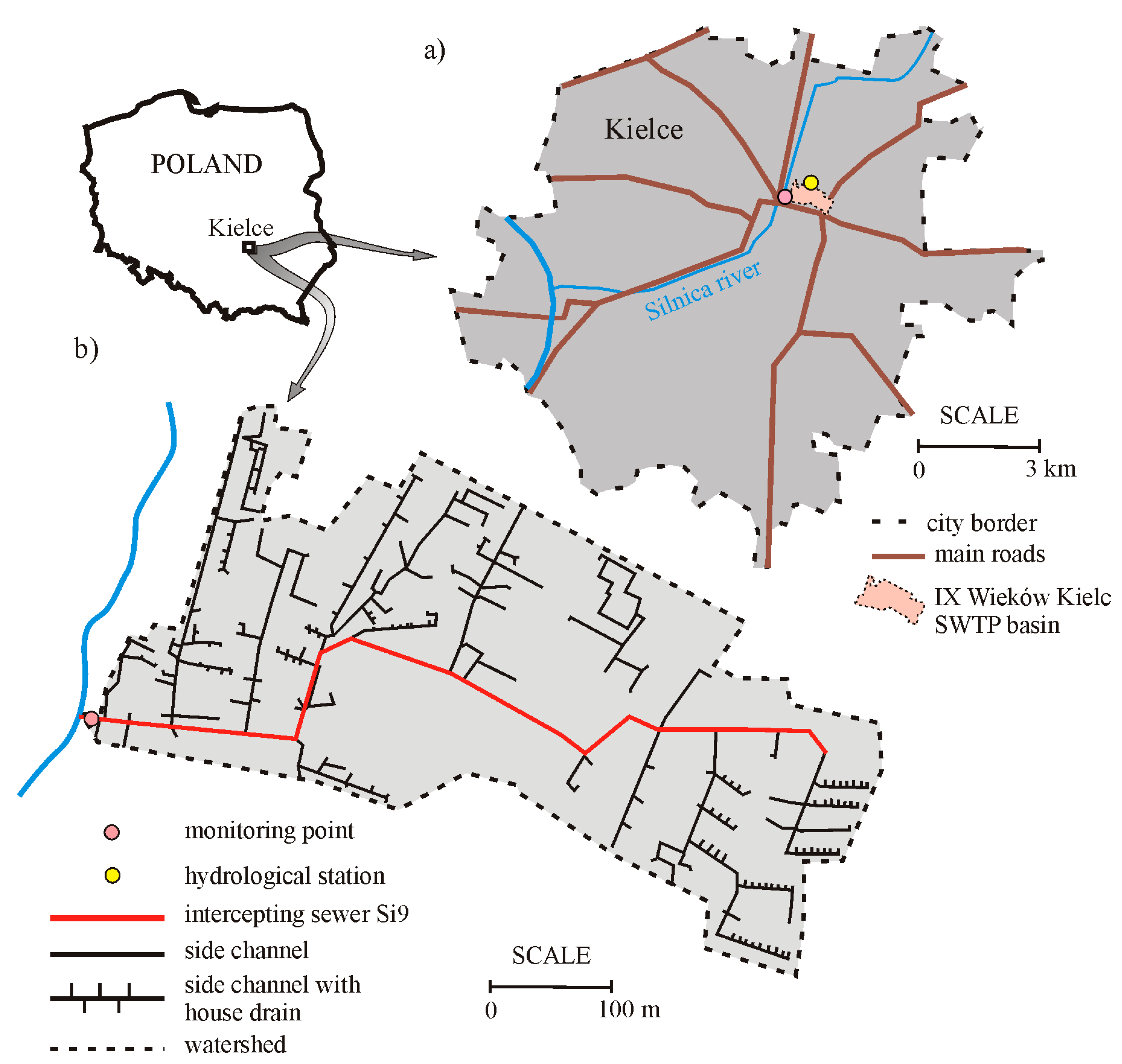
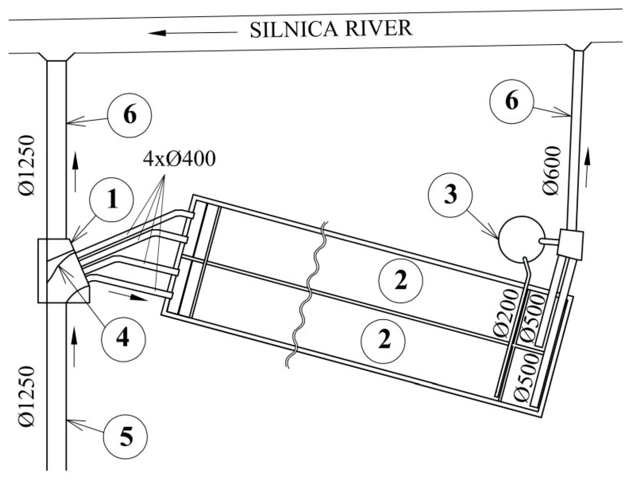
2.1. Study Area

The studies were performed in the catchment of collector Si9, with an area of A = 62 ha, located in the central-eastern part of the city of Kielce (Figure 1). In terms of development, the catchment area is primarily covered by housing estates, public buildings, and arterial and secondary streets. The highest point of the catchment area is located at 271.20 m a.s.l., and the lowest at 260.00 m a.s.l. The average slope of the catchment is 0.71%. The catchment consists mainly of green lands, which constitute 47.17% of its area. The remaining 52.83% includes roads and streets (17.66%), roof surfaces (14.27%), parking spaces (11.20%), pavements (8.41%), and asphalt school playgrounds (1.29%). Overall, impervious areas with a high runoff coefficient constitute 52% of the total catchment area, which indicates its typically urban character. The diameter of the main sewer, which is over 1.5 km in length, ranges from 600 to 1250 mm, and the diameters of 17 lateral sewers vary from 300 to 1000 mm [34,35].

Before being discharged to the receiver (the Silnica river), the stormwater is pre–treated at the stormwater treatment plant (SWTP) located in IX Wieków Kielc street (Figure 2). The facility consists of two horizontal settling tanks with a length of 30 m each, and a coalescence separator with a diameter of 3.0 m.

2.2. Measurements of Precipitation and Flow Intensity

Measurements of atmospheric precipitation were taken with a Total Rain weighing Sensor TRwS by BMsonic at 1 min frequency and 0.001 mm resolution. The rain gauge, which meets the requirements set by the World Meteorological Organization (WMO), was located approx. 1.0 km from the Si9 collector outlet (Figure 1).

According to the manufacturer’s specifications, the relative measurement accuracy is ±1%. WMO-No. 8 [36] guidelines state that weight-based rain gauges offer sufficient accuracy and are recommended for continuous recording of precipitation. Investigations conducted by Licznar [37] confirmed the high potential of this type of rain gauge for high accuracy measurements compared with laser disdrometers.

Additionally, the amount of stormwater was measured using a ISCO AV 2150 modular flow meter from Teledyne ISCO. It was set up in separation chamber (1) located in canal inlet (5) to the SWTP (Figure 2). The meter’s principle of operation is based on the measurements of the water column pressure and the mean flow rate in the canal, recorded with an AV probe. The measurement frequency during the peak runoff event ranged from 15 to 30 s, and from 1 to 5 min prior to the event, depending on the instrument set-up.

Further analyses were based on the results of tests on stormwater amount and quality for the period between May 2017 and August 2018 (13 precipitation-runoff events of the spring–autumn season). High water stage events due to thawing were not taken into account. The parameters of the events and precipitation characteristics are listed in

Table 1. Parameters of the observed high water stages and precipitation.

No.	Ptd=10	P	td	q	Pa	Qmax	Vc	tp	tbd	Number of Samples
	mm	mm	min	L·s−1·ha	mm	m3·s−1	m3	min	h
1	-	2.6	360	1.20	1.3	0.313	632	50.0	54.0	8
2	1.8	2.1	54	6.48	3.6	0.360	510	23.5	25.0	8
3	-	6.6	480	2.29	2.6	0.076	200	32.0	0.6	8
4	0.5	1.1	48	3.82	1.4	0.094	263	33.5	3.1	12
5	0.5	5.2	424	2.04	2.8	0.274	1232	82.0	28.4	12
6	0.4	1.3	78	2.78	3.8	0.046	212	45.0	127.0	8
7	1.3	3.6	92	6.52	1.3	0.111	327	16.0	132.0	9
8	0.9	6.6	298	3.69	8.1	0.148	1173	162.5	137.0	24
9	0.5	3.1	170	3.04	6.6	0.101	687	122.0	6.0	24
10	4.6	8.3	24	57.65	3.6	0.173	425	29.5	43.3	9
11	2.9	5.4	56	16.07	2.8	0.277	684	19.0	71.2	9
12	0.7	4.0	168	3.97	5.4	0.140	580	26.0	8.2	14
13	0.7	6.3	106	9.91	4.8	0.312	755	78.0	10.2	14

P_td=10—10-min amount of precipitation, P—total amount of precipitation, t_d—duration of rain, q—intensity of rain, P_a—depth of the previous rainfall, Q_max—maximum flow rate, V_c—total high water stage volume, t_p—total duration of the runoff event, t_bd—inter-event (rainless) time.

.

2.3. Collection of Stormwater Samples

Stormwater samples were collected using an ISCO 6712 portable sampler by Teledyne ISCO, which satisfies the requirements of the United States Environmental Protection Agency (US EPA), equipped with 24 bottles, each having a volume of 0.5 dm³. The device was activated when the stream of effluents reached a depth of 3 cm, recorded by a probe measuring the canal filling. It should be mentioned that yearly observations indicate that a certain amount of flow, estimated to be about 2 dm³·s⁻¹, is always found in the canal due to groundwater seepage. The time step in stormwater sampling ranged from 5 to 15 min, and was set depending on the predicted duration of the precipitation event. The location of the stormwater sampling site is shown in Figure 1.

2.4. Determination of the Physicochemical Properties of Samples

Stormwater samples were not preserved, but they were transported directly to a laboratory in order to determine their selected physicochemical parameters. Laboratory tests on the stormwater quality concerned selected HMs (Ni, Cu, Cr, Zn, Pb, and Cd) and TSS. The HM concentrations were examined using the atomic absorption spectroscopy (ASA) method with flame atomization following the PN-EN ISO 8288:2002 standard [38]. Prior to content determination, the samples were mineralized in accordance with the EN ISO 15587-1:2005 standard [39] methodology using a microwave oven (Multiwave 3000). TSS were assessed following the PN-EN 872:2007 standard [40] using filtration through glass fiber filters.

2.5. Analysis of Data

Instantaneous loads of pollutants specified in sampling were calculated using the formula:

$$l=c_m·Q \left(\mathrm{kg}·{\mathrm{s}}^{-1}\right)$$

(1)

where: c_m is the measured concentration of pollutants (kg∙m⁻³), Q is the stormwater flow rate (m³∙s⁻¹).

To calculate cumulative loads of pollutants in the peak runoff wave, it is necessary to know the concentration at an arbitrary moment of the event duration. For this purpose, the measured values of the concentration of pollutants were smoothed using the selected equation. The coefficient of determination, R², was used to measure the accuracy of the fit of the regression to the empirical data. It was possible to find concentration values beyond the time intervals in which stormwater was sampled for analyses. The values of approximated loads of total suspended solids at time t_i of the peak runoff event were calculated from the formula:

$$l_i=Q_i·c_i \left(\mathrm{kg}·{\mathrm{s}}^{-1}\right)$$

(2)

where: Q_i is the stormwater flow rate in time t_i (m³∙s⁻¹), c_i is the approximated concentration of pollutions in time t_i (kg∙m⁻³).

Based on measurements, pollution loads (TSS and HMs) washed out of the catchment surface were calculated with the formula:

$$M={\displaystyle \sum }_{i=1}^n\frac{\left(l_i+l_{i+1}\right)}{2}·\Delta t \left[\mathrm{kg}\right]$$

(3)

where l_i,_i+1 is the approximated load of pollutants for time t_i and time t_i+1 (kg·s⁻¹), calculated from Formula (2), n is the number of time steps, and Δt is the time step, calculated as Δt = t_i+1 − t_i (s).

The cumulative volume for a given event was calculated from the formula:

$$V={\displaystyle \sum }_{i=1}^n\frac{\left(Q_i+Q_{i+1}\right)}{2}·\Delta t \left[{\mathrm{m}}^3\right]$$

(4)

where Q_i, Q_i+1–flow rates in time t_i and time t_i+1 (m³∙s⁻¹).

Then, pollution loads made it possible to generate pollutographs for the analyzed precipitation events in the form of M/M_c = f(x = V/V_c). In the analyses, the variation was extrapolated by a power Function (5) and an exponential Function (6) [7].

$$F\left(x\right)=x^a$$

(5)

$$F\left(x\right)=\frac{1-e^{-kx}}{1-e^{-k}}$$

(6)

where a and k are the washout coefficients.

In both cases, the values of a and k were determined with the Levenberg–Marquardt method [41], using the STATISTICA software. Subsequently, by means of t-Student statistics, it was checked whether the analyzed variables (k, P, t_d, q, Q_max, V_c, h, t_p, t_bd) had normal distributions. If these variables showed normal distribution, a matrix of Pearson’s linear correlation was generated for p = 0.05. If, however, this was not the case, a matrix of gamma rank correlation was created for p = 0.05. This method is recommended when the statistical samples are small [41], which was the case because 13 precipitation events were taken into account. The results of correlation analyses were used to select variables producing a significant impact on the pattern of variation of washout coefficients (a and k), which was approximated by the following equation:

$$k=\alpha ·exp\left(-\beta ·z\right)$$

(7)

where α and β are the empirical parameters determined using the Levenberg–Marquardt method, and z is the analyzed variable.

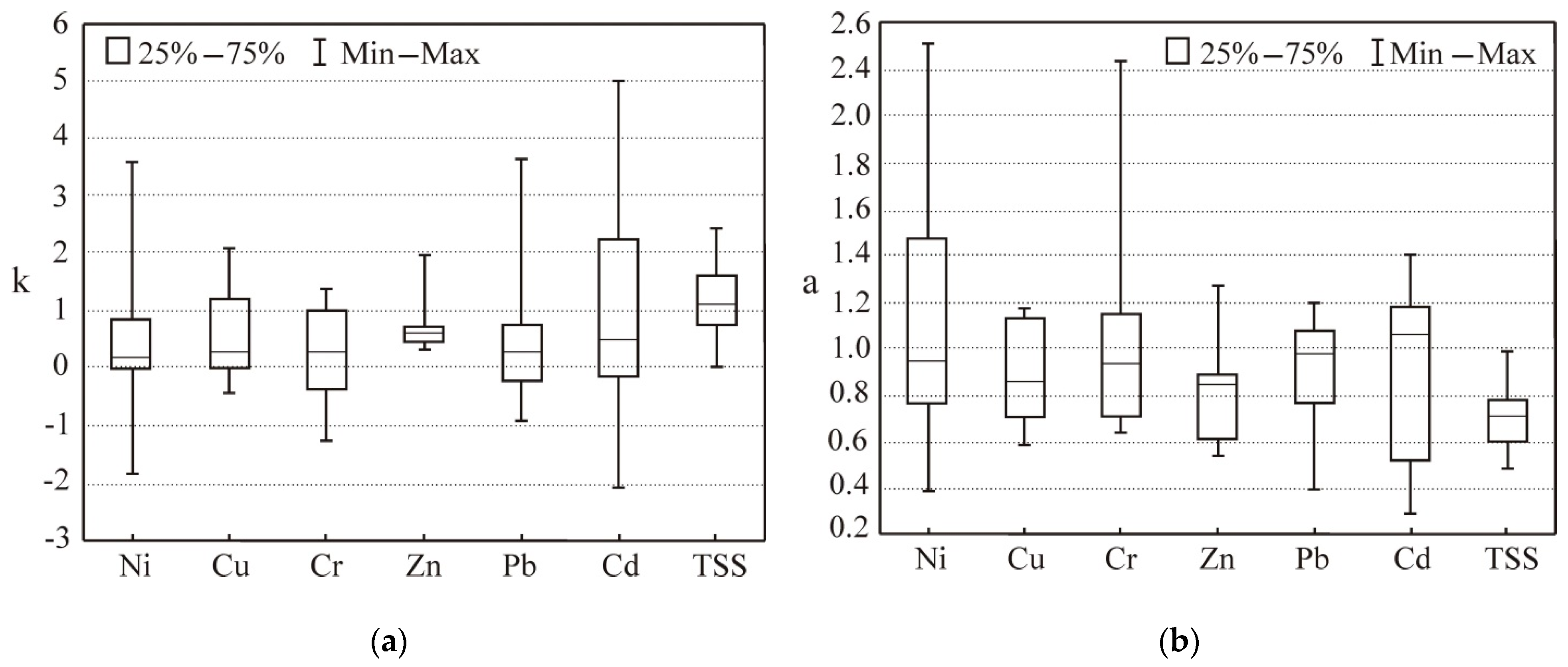
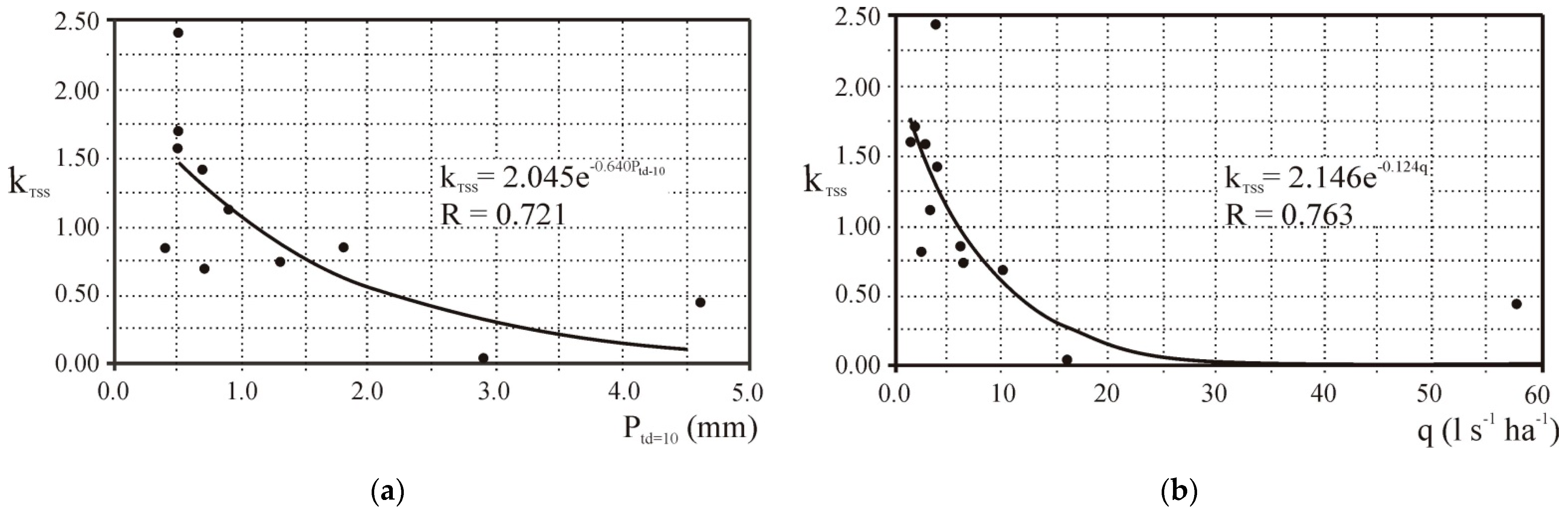
3. Results and Discussion

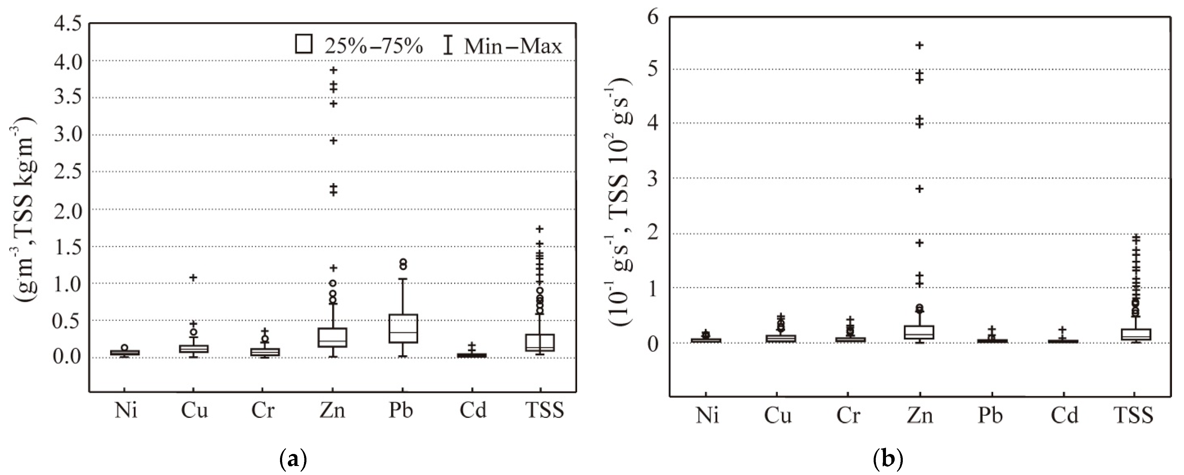
3.1. Results of Physicochemical Analyses

The quantity of TSS is one of the most important indicators of stormwater pollution. Although solids themselves can adversely affect the aquatic environment of the receiver, they also act as media for transporting other types of pollutants, including HMs. The differences in the specific surface area of the of suspended solids particles result in their various sorption properties. The processes of co-precipitation and sorption on the surface of clay minerals and on organic particles significantly contribute to a decrease in the migration of trace metal compounds in the water environment [42,43,44]. Numerous studies indicate that the most frequently analyzed HMs are Ni, Cu, Cr, Zn, Pb, and Cd [45,46,47,48,49,50,51,52,53,54,55,56,57].

The investigations into the concentrations and temporary loads of TSS (C_TSS and M_TSS; Figure 3) in the analyzed period showed the results were in the ranges of 40–1735 g·m⁻³ and 0.54–191.85 g·s⁻¹, with median values of 120 g·m⁻³ and 7.54 g·s⁻¹, respectively. Regarding TSS concentrations, the values are similar to those observed in urban areas in Germany (29–1535 g·m⁻³) [45], and in Santa Monica (12–1400 g·m⁻³) [46]. The values resemble the data for high density residential areas (55–1568 g·m⁻³) [47], and car parks and commercial land use (42–2185 g·m⁻³) [48]. Maximum values, however, are over three times lower than in discharges from motorways and major roads (5700 g·m⁻³), or urban, suburban, and residential roads (5400 g·m⁻³) [47], as shown by European data. TSS concentrations in an interval between the 1st and the 3rd quartiles (86.5–291.5 g·m⁻³) are close to the ranges specified by Gnecco et al. [49] for Genoa in Italy (15–377 g·m⁻³), Gasperi et al. [50] for Paris in France (119–254 g·m⁻³), and Taebi and Droste [51] for Isfahan in Iran (43–467 g·m⁻³).

Heavy metals, found primarily in the airborne particulate matter, are particularly hazardous substances. Deposited on the ground together with particulate matter, they are then washed off the catchment and transported, with the stormwater, into the wastewater receiving body. High concentrations of zinc, lead, and nickel in the stormwater result from the widespread use of these elements in the automotive and fuel industries. The presence of copper and chromium in the atmosphere is mainly caused by coal combustion and industrial activities [35,53,58].

The data in Figure 3 show that, for all tested HMs, but in particular for Cu, Zn, and Cd, the values of concentrations and temporary loads within a range between the 25th and 75th percentiles are several times lower than the recorded maxima. The highest concentrations and temporary loads were found for Zn and Pb, for which the maximum values reached the respective levels of 3.87 g·m⁻³ and 0.547 g·s⁻¹, and 1.28 g·m⁻³ and 0.267 g·s⁻¹. The lowest maxima concetrations and loads were observed in the case of Ni and Cd, namely, 0.11 g·m⁻³ and 0.012 g·s⁻¹, and 0.16 g·m⁻³ and 0.024 g·s⁻¹, respectively. The high concentrations of Zn in the studied catchments result from the relatively large cumulative area of the roofs [59] in the study catchment.

Concentrations of Zn and Cd that are harmful to plants, water microorganisms, and fish are extremely low; actual values are smaller than 0.1 g·m⁻³ [52]. Regarding Zn, the range of values between the first and the third quartiles (0.13–0.38 g·m⁻³) exceeds the value above, resulting in the toxicity of stormwater examined. The high Zn values fell within the range specified by Królikowski et al. [53] for Białystok (0.20–6.00 g·m⁻³) and Djukić et al. [54] for Belgrade (0.28–6.20 g·m⁻³). The remaining Zn values were close to the upper ranges determined by Brombach and Fuchs [45] of 3.56 g·m⁻³, and Gan et al. [55] of 4.40 g·m⁻³. Comparing the Cd and Pb concentrations with the findings of other researchers [51,55,56], it can be seen that the values specified by them are in most cases considerably lower than not just the maximum values, but also the medians reported in this study. The observed maximum Pb content is similar to the upper limit established for motorways and major roads [47].

The median of concentrations for Cu (0.09 g·m⁻³) was almost twice as high as for Cr (0.05 g·m⁻³). The ranges of Cu and Cr concentrations between the lower and the upper quartiles (0.06–0.15 and 0.03–0.11 g·m⁻³, respectively) are within the intervals specified for high density residential areas [57], similar to the maximum value of Ni concentration.

When sizing facilities in stormwater treatment plants, the pollutant loads seem to be a more reliable criterion than pollutant concentrations. The same holds true for the assessment of the impact of pollutants on the water and soil environment of the stormwater receivers, namely, watercourses, or the ground. The pollutant loads in the observed high-water stages varied considerably (

Table 2. Statistical characteristics of pollutant loads washed out of the catchment area.

Pollution	Load
	Range	Mean	Standard Deviation	Coefficient of Variation (%)
	(10−3·kg), * (kg)
Ni	0.54–50.15	15.52	13.17	84.85
Cu	19.50–94.44	50.83	25.00	49.18
Cr	13.25–68.54	28.74	18.72	65.13
Zn	52.84–1452.00	251.95	424.62	168.53
Pb	16.86–412.71	211.81	132.51	62.56
Cd	0.60–19.73	10.72	6.68	62.31
TSS *	22.90–796.00	160.23	220.57	137.65

* HMs concentrations are in [10⁻³·kg] and TSS concentrations are in [kg].

).

The highest variation in loads was observed for Zn and TSS. The values of the coefficient of variation greatly exceeded 100% for these pollutants. Conversely, the lowest variation in loads was observed for Cu. In this case, the value of the coefficient of variation was lower than 50%. The mean values of pollutant loads (HM) flowing out of the analyzed catchment area during individual high water events can be put in the following decreasing sequence: Zn > Pb > Cu > Cr > Ni > Cd. The results are congruent with the findings of other researchers for urban agglomerations of various sizes [57].

The data collated in

Table 3. The matrix of correlation between the analyzed parameters.

Variable	MTSS	MNi	MCu	MCr	MZn	MPb	MCd
P	0.127	0.428	0.048	−0.238	0.048	−0.048	0.238
td	0.127	0.428	0.428	0.333	0.048	0.333	0.238
Ptd=10	0.098	0.100	0.100	0.100	0.500	0.200	0.100
q	−0.091	0.048	−0.143	−0.428	0.048	−0.048	0.048
Qmax	0.454	−0.048	0.333	0.238	0.524	0.428	0.333
Vc	0.454	0.524	0.524	0.238	0.333	0.428	0.524
tp	0.296	0.048	0.428	0.143	0.048	0.333	0.428
tbd	−0.054	−0.048	−0.048	−0.143	−0.048	0.143	−0.048

also indicate that the magnitude of the TSS, Ni, Cu, Zn, and Cd loads flowing out of the studied catchment area depends directly proportionally on the total volume of surface runoff (V_c), or the maximum flow rate.

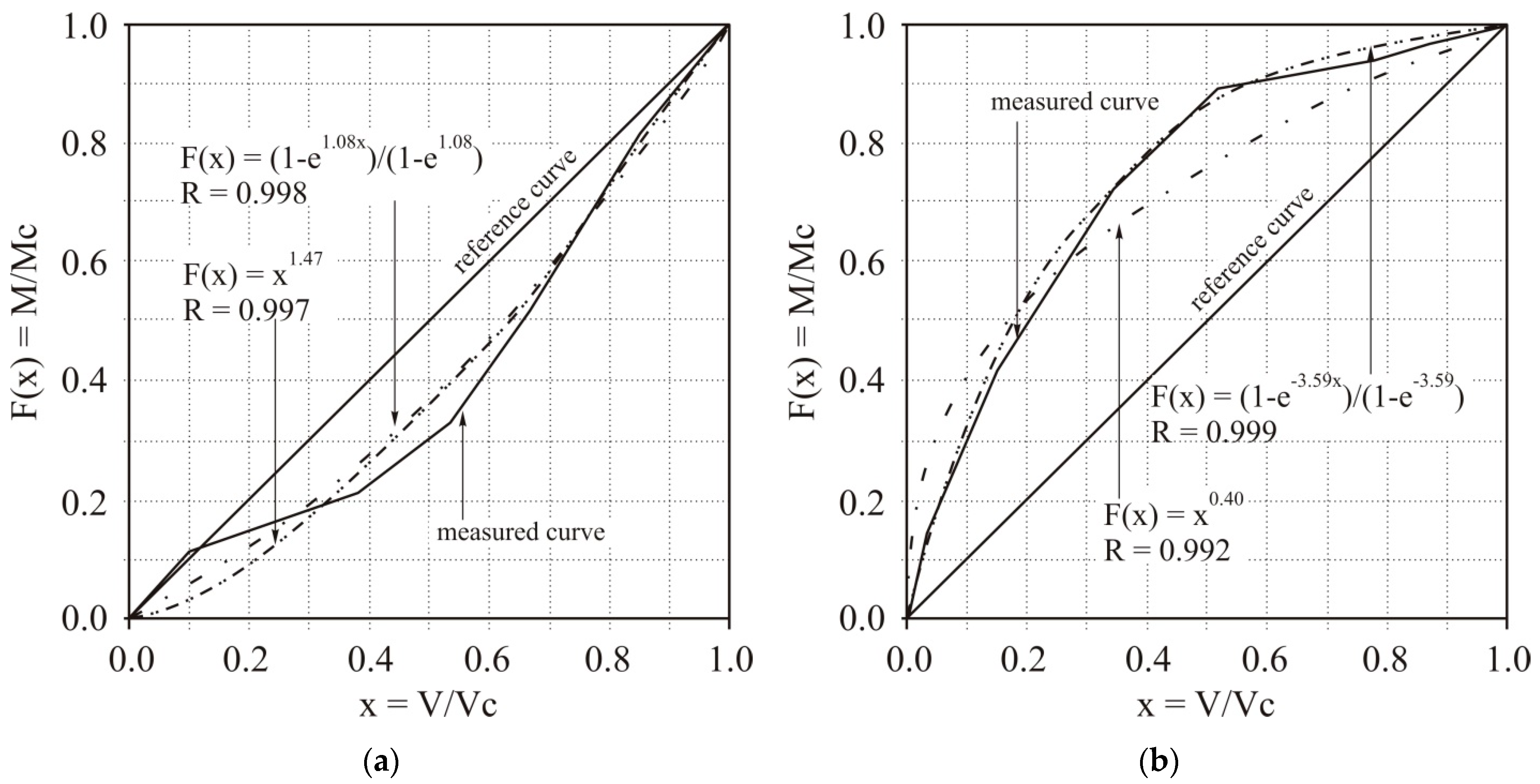
3.2. The Impact of Precipitation Characteristics and Parameters of the Runoff Hydrograph on the Value of the Washout Coefficient

When the evaluation of the performance of technological facilities of stormwater treatment plants (e.g., oil-derivative separators, settlement tanks of suspended solids) is based on average values of pollutant indicators, it is not possible to optimize those facilities. The most polluted first flush should be directed to them, whereas the remaining runoff does not require that procedure. Polish legal regulations allow stormwater discharge to a receiver without pre-treatment, if the concentration of total suspended solids and oil-derivatives does not exceed 100 and 15 mg·dm⁻³, respectively. Consequently, the time and manner of collecting samples becomes an issue of key importance. With respect to the protection of a stormwater receiving body against pollution with, e.g., non-biodegradable heavy metals, a reliable analysis of variation in the concentrations of individual pollutants is required. More importantly, however, it is the magnitude of pollutant loads discharged into the environment that counts. As a result, when modeling stormwater quality, it is necessary to precisely determine the variation range of washout coefficients because those data affect the simulation reliability.

In the manuscript, precipitation depths were measured with a rain gauge. Average rainfall intensity q = P/t_d was determined for individual rainfall events. The outflow hydrograph volume was determined based on the measured flow values. The developed model was validated for three rainfall events accounted for in 2021. In the first event (p = 4.2 mm, t_d = 140 min, and V_c = 712 m³), in the second event (p = 6.0 mm, t_d = 100 min, and V_c = 968 m³), and in the third event (p = 8.0 mm, t_d = 80 min, and V_c = 1208 m³), the respective values of the washout coefficient (k) were obtained: 1.05, 0.50 and 0.22.

Exemplary pollutographs developed for Ni are shown in Figure 4. The pattern of variation of the function was approximated by means of a power function and an exponential function. The analysis of the figure and of the values of correlation coefficients (R) indicates that Equation (6) describes the measured pattern of variation of the curve F(x) = f(V/V_c) slightly better than Equation (5) M/M_c = f(V/V_c). In seven cases, calculations performed for the remaining precipitation events demonstrated similar relationships both for TSS and for the studied HMs. Values of the coefficients of determination ranged from 0.900 to 0.999 in cases when Equation (6) was used to describe the observed variation F(x) = f(V/V_c) of the studied pollutants, and from 0.864 to 0.999 when this variation was described by means of Equation (5).

The analysis of equations shown in Figure 4 also indicates that the washout coefficient (a) takes on positive values, whereas the coefficient (k) may take on both positive and negative values. In this case, when k > 0, the first flush phenomenon occurs; that is, during 30% of the initial runoff volume, 80% of the total pollutant load is transported [60]. On the contrary, when k < 0, the so-called last flush phenomenon is observed [60]. The range of variation of washout coefficients (a and k) for the investigated pollution indicators can be seen in Figure 5. The mean value of the washout coefficient (k) for HMs ranges from 0.10 to 0.60, whereas for TSS this value is higher and equals 1.08 (Figure 5a). The highest variation in the coefficient k was found for Cd, whereas the lowest variation was identified for Zn. With respect to the majority of the investigated trace elements, the washout coefficient (k) takes on both positive and negative values. The only exception is found for Zn, in which case the minimum value of k equals 0.31. Regarding TSS, the minimum value of the coefficient (k) is 0.036.

For most of the investigated HMs, the mean value of the washout coefficient (a) ranges from 0.8 to 1.0, and is slightly higher than one only for Cd (1.06) (Figure 5b). With respect to mineral pollutants, the coefficient (a) mean value is lower than that determined for HMs, and equals 0.73. Figure 5b also demonstrates that the highest variation in the coefficient (a) values for the analyzed metals was observed in the case of Ni (0.39–2.52), and the lowest variation was observed for Cu (0.59–1.19).

The occurrence of strong correlations between runoff hydrographs characteristics and the values of pollutant washout coefficients indicates relationships holding between the analyzed parameters. Correlations also provide valuable information on factors decisive for the washout and transport of the pollutants studied, namely HMs and TSS. The analyses demonstrate a strong correlation relationship between the washout coefficient for TSS (k_TSS) and the rainfall intensity. Additionally, the presence of a statistically significant relationship for a p-value = 0.05 was observed between (k_TSS) and total precipitation (P), and also 10-min precipitation (P_td=10) (

Table 4. The matrix of correlation between the analyzed parameters.

Variable	kTSS	kNi	kCu	kCr	kZn	kPb	kCd
P	−0.509	−0.289	−0.289	−0.333	−0.067	−0.067	0.022
td	0.409	−0.200	−0.067	−0.111	−0.200	−0.022	0.067
Ptd=10	−0.658	−0.257	0.029	0.086	0.371	−0.086	−0.143
q	−0.773	−0.155	−0.067	0.067	0.244	0.156	−0.022
Qmax	−0.309	0.155	0.155	0.200	0.111	0.022	−0.067
Vc	0.136	−0.066	−0.111	−0.067	0.022	0.111	0.378
tp	0.111	−0.363	−0.409	−0.272	−0.272	−0.182	0.182
tbd	0.382	−0.111	−0.155	−0.289	−0.022	−0.556	−0.289

). An increase in the precipitation intensity is accompanied by an increase in the amount of stormwater flowing over the surface to the drainage systems. This co-occurs with an increase in the flow capacity to transport the grains of mineral suspended solids of specified sizes. Regarding the investigated HMs, only a minor relationship was observed between the washout coefficient of Pb (k_Pb) and the dry period length (t_bd) (Table 4). The occurrence of significant regressive relationships between the washout coefficient (a) and the precipitation characteristics, or the parameters of the hydrograph shape, was not observed in any of the analyzed cases. The lack of regressive relationships between the washout coefficients (a and k) for HMs and the calculated characteristics of high water stages or precipitation may indicate that other factors, not accounted for in the study, are involved. The presence of those factors, including, among others, surface type and runoff path length, may affect the nature of this phenomenon.

The values of the coefficients of correlation between individual parameters of rainfall events and the resulting high water stages in the sewerage systems, and the calculated pollutant washout coefficient (Table 4) and pollutant loads (Table 3), were found to be low. The reason for this may lie in the fact that the studied catchment is nonhomogeneous in character. The quality of stormwater may be affected by the mixing of stormwater streams from individual side channels along the length of the main collector. These collect stormwater from sub-catchments showing different types of land use. The results are confirmed by investigations for nonhomogeneous catchments reported in [6]. Regarding homogeneous catchments, strong relationships are most often found to hold between precipitation dynamics and pollutant washout [18]. Consequently, it is necessary to continue investigations concerning a catchment showing diversified characteristics. The goal would be to validate the results obtained, and to develop universal relationships that could be applicable in a wider context.

Based on the data in Table 4, an attempt was made to approximate the values of the washout coefficient for TSS (k_TSS) according to Formula (7). When describing the variation in the washout coefficient (k_TSS), two parameters were used: q and P_td=10, as the ones most strongly correlated with the endogenous variable. On the basis of the data in Figure 6, it was possible to estimate, with satisfactory accuracy, the values of the washout parameters for TSS (k_TSS). Additionally, the calculations demonstrated that empirical parameters included in the equations k_TSS = f(P_td=10) and k_TSS = f(q) are statistically significant for a p-value = 0.05, and they explain 52% and 58% of the observed variation, respectively.

Observations on statistically significant relationships between the washout coefficient for TSS and mean precipitation intensity and magnitude made by the authors are congruent with the findings reported by Christian et al. (2007) [61]. In the latter study, which concerned developed areas and a vehicle disassembly plant, an exponential function was used to describe the relationship. A good fit was achieved. Chow and Yusop [62], who investigated urban catchments, observed the presence of strong regressive relationships between parameters describing the precipitation properties and the amount of TSS discharged from the catchment surface. This indicates a possibility to describe the TSS washout process as a function of precipitation parameters and, as a result, to determine the load of suspended solids flowing into stormwater drainage systems. Information on the quantity of suspended solids transported in high water stages is of crucial importance for the design of stormwater treatment plants. This translates into the protection of receiver waters against pollution.

The calculations performed for the study refer to the catchment under analysis. They should be extended substantially in order to determine general relationships. The latter need to account for the characteristics of different urban catchments, and also precipitation characteristics, including rainfall time distribution and intensity.

4. Conclusions

Calculations given in this paper indicate that the washout coefficient does not assume a constant value. This is important when modeling the process of pollutant washout from the land surface. In this context, Equation (6), which describes the pollutant distributions in the catchment outflow hydrograph for long periods (1, 2, 5, … 30 years), is attributed a different meaning. Formula (6), together with the stormwater outflow model, can be used to analyze pollutant distributions in each precipitation event. This can provide a basis when sizing the retention reservoir or stormwater treatment plant. These factors are important for the catchment management, and the control of stormwater quality and its impact on the receiver environment.

The calculations performed for this study demonstrated that, to describe the pollutograph M/M_c = f(V/V_c), it is possible to use a power function and an exponential function. It is recommended to employ the latter, because, as discussed in the paper, the washout coefficient (k) depends on precipitation characteristics and parameters of the runoff hydrograph.

The mean value of the washout coefficient (k) for the examined HMs ranged between 0.10 and 0.60, and the highest variation was found for Cd, and the lowest for Zn. Regarding TSS, the mean value of k coefficient was 1.08.

The mean value of the washout coefficient (a) for most HMs ranged from 0.8 to 1.0, except for Cd (a = 1.06). With respect to TSS, the coefficient was 0.73. The highest (a) coefficient variation was observed for Ni, and the lowest for Cu.

Making the washout coefficient dependent on precipitation data leads to improvement in the congruence of the simulation results with measurements, when compared with the majority of the models currently used. In the future, these findings may be relied on at the stage of model development.

The distribution of rainfall intensity (q), and therefore the total amount of precipitation (P) and 10-min rainfall (P_td=10), affect the washout coefficient for TSS (k_TSS) removed from the analysed urban catchment area. It was shown that the value of the washout coefficient for TSS (k_TSS) was reduced with an increase in rainfall intensity q or P_td=10.

As precipitation intensity increases, the shape of M/M_c = f(V/V_c) becomes closer to the reference curve, resulting in the disappearance of the first flush phenomenon.

With respect to the analyzed HMs (Ni, Cu, Cr, Zn, Pb, and Cd), the only statistically significant effect of the dry period on the washout coefficient was observed for Pb (k_Pb). The remaining cases did not indicate an impact of precipitation characteristics, or the parameters of the runoff hydrograph on the washout parameters for HMs.

The calculations reported in the study also imply a statistically significant effect of surface runoff (V_c) on the load of washed out TSS, Ni, Cu, and Cd. Additionally, the 10-min precipitation (P_td=10) and the maximum flow rate (Q_max) have a statistically significant impact on the load of Zn washed out of the surface of the catchment area.

The analyses confirmed the complex dynamics of HMs washout in the examined catchment. For most cases, strong statistical relations were not found. That statement is not equivalent to the fact that such relationships do not exist. However, it indicates the process is highly non-linear in character. Consequently, it seems reasonable that further analyses employing more advanced computational tools should be conducted.

References

1. Hossain, I.; Imteaz, M.; Gato-Trinidad, S.; Shanableh, A. Development of a Catchment Water Quality Model for Continuous Simulations of Pollutants Build-up and Wash-off. Int. J. Civ. Environ. Eng. 2010, 2, 210–217. [Google Scholar]
2. Sartor, J.D.; Boyd, G.B.; Agardy, F.J. Water pollution aspects of street surface contaminants. Contract 1972, 14, 921. [Google Scholar]
3. Bertrand-Krajewski, J.L.; Chebbo, G.; Saget, A. Distribution of pollutant mass vs volume in stormwater discharges and the first flash phenomenon. Water Resour. 1998, 32, 2341–2356. [Google Scholar]
4. Osuch-Pajdzińska, E.; Zawilski, M. Model of Storm Sewer Discharge. I: Description. J. Environ. Eng. 1998, 124, 593–599. [Google Scholar] [CrossRef]
5. Osuch-Pajdzińska, E.; Zawilski, M. Model for Storm Sewer Discharge. II: Calibration and Verification. J. Environ. Eng. 1998, 124, 600–611. [Google Scholar] [CrossRef]
6. Berretta, C.; Gnecco, J.; Lanza, L.G.; Berbera, P. An Investigation of Wash-Off Controlling Parameters at Two Urban Sites in the Town of Genova. 2007. Available online: http://documents.irevues.inist.fr/bitstream/handle/2042/25296/1425_254berretta.pdf?sequence=1 (accessed on 15 April 2021).
7. Egodawatta, P. Translation of Small-Plot Scale Pollutant Build-Up and Wash-Off Measurements to Urban Catchment Scale. 2007. Available online: https://eprints.qut.edu.au/16502/1/Prasanna_Egodawatta_Thesis.pdf (accessed on 15 April 2021).
8. Alley, W.M.; Smith, P.E. Estimation of accumulation parameters for urban runoff quality modeling. Water Resour. Res. 1981, 17, 1657–1664. [Google Scholar] [CrossRef]
9. Lee, J.Y.; Kim, H.; Kim, Y.; Han, M.Y. Characteristics of the event mean concentration (EMC) from rainfall runoff on an urban highway. Environ. Pollut. 2011, 159, 884–888. [Google Scholar] [CrossRef]
10. Yuan, Q.; Guerra, H.B.; Kim, Y. An Investigation of the Relationships between Rainfall Conditions and Pollutant Wash-Off from the Paved Road. Water 2017, 9, 232. [Google Scholar] [CrossRef]
11. Vezzaro, L.; Sharma, A.K.; Mikkelsen, P.S. Model-Based Comparison of Strategies for Reduction of Stormwater Micropollutants Emission. 2013. Available online: https://hal.archives-ouvertes.fr/hal-03303544/document (accessed on 15 April 2021).
12. Zhao, H.; Li, X. Understanding the relationship between heavy metals in road-deposited sediments and washoff particles in urban stormwater using simulated rainfall. J. Hazard. Mater. 2013, 246, 267–276. [Google Scholar] [CrossRef] [PubMed]
13. Deletic, A.; Maksimovic, C.; Loughreit, F.; Butler, D. Modelling the Management of Street Surface Sediments in Urban Runoff. 1998. Available online: https://www.academia.edu/2860576/Modelling_the_management_of_street_surface_sediments_in_urban_runoff (accessed on 15 April 2021).
14. Avellaneda, P.; Ballestero, T.; Roseen, R.; Houle, J.; Linder, E. Bayesian Storm-Water Quality Model and Its Application to Water Quality Monitoring. J. Environ. Eng. 2011, 137, 541–550. [Google Scholar] [CrossRef] [Green Version]
15. Chen, J.; Adams, B.J. Analytical Urban Storm Water Quality Models Based on Pollutant Buildup and Washoff Processes. J. Environ. Eng. 2006, 132, 1314–1330. [Google Scholar] [CrossRef]
16. Dotto, C.B.; Mannina, G.; Kleidorfer, M.; Vezzaro, L.; Henrichs, M.; McCarthy, D.; Freni, G.; Rauch, W.; Deletic, A. Comparison of different uncertainty techniques in urban stormwater quantity and quality modelling. Water Res. 2012, 46, 2545–2558. [Google Scholar] [CrossRef]
17. Fraga, I.; Cea, L.; Puertas, J.; Suárez, J.; Jiménez, V.; Jácome, A. Global Sensitivity and GLUE-Based Uncertainty Analysis of a 2D-1D Dual Urban Drainage Model. J. Hydrol. Eng. 2016, 21, 04016004. [Google Scholar] [CrossRef]
18. Perera, T.; McGree, J.; Egodawatta, P.; Jinadasa, K.; Goonetilleke, A. Catchment based estimation of pollutant event mean concentration (EMC) and implications for first flush assessment. J. Environ. Manag. 2021, 279, 111737. [Google Scholar] [CrossRef]
19. Rossmann, L.A. Storm Water Management Model, User’s Manual, Version 5.1. National Risk Management Research Laboratory Office of Research and Development; U.S. Environmental Protection Agency: Cincinnati, OH, USA, 2004.
20. Tuomela, C.; Sillanpää, N.; Koivusalo, H. Assessment of stormwater pollutant loads and source area contributions with storm water management model (SWMM). J. Environ. Manag. 2019, 233, 719–727. [Google Scholar] [CrossRef]
21. Egemose, S.; Petersen, A.B.; Sønderup, M.J.; Flindt, M.R. First Flush Characteristics in Separate Sewer Stormwater and Implications for Treatment. Sustainability 2020, 12, 5063. [Google Scholar] [CrossRef]
22. Verdaguer, M.; Clara, N.; Gutierrez, O.; Poch, M. Application of Ant-Colony-Optimization algorithm for improved management of first flush effects in urban wastewater systems. Sci. Total. Environ. 2014, 485, 143–152. [Google Scholar] [CrossRef] [PubMed]
23. Mrowiec, M.; Kamizela, T.; Kowalczyk, M. Occurrence of first flush phenomenon in drainage system of Częstochowa. Environ. Prot. Eng. 2009, 35, 73–80. [Google Scholar]
24. Deletic, A. The first flush load of urban surface runoff. Water Res. 1998, 32, 2462–2470. [Google Scholar] [CrossRef]
25. Sansalone, J.J.; Buchberger, S.G. Partitioning and First Flush of Metals in Urban Roadway Storm Water. J. Environ. Eng. 1997, 123, 134–143. [Google Scholar] [CrossRef]
26. Stahre, P.; Urbonas, B. Stormwater Detention: For Drainage, Water Quality and CSO Management, 1st ed.; Prentice Hall PTR: Hoboken, NJ, USA, 1990. [Google Scholar]
27. Kim, I.; Ko, S.-O.; Jeong, S.; Yoon, J. Characteristics of washed-off pollutants and dynamic EMCs in parking lots and bridges during a storm. Sci. Total. Environ. 2007, 376, 178–184. [Google Scholar] [CrossRef]
28. McCarthy, D.T. A traditional first flush assessment of E. coli in urban stormwater runoff. Water Sci. Technol. 2009, 60, 2749–2757. [Google Scholar] [CrossRef]
29. Kang, J.-H.; Kayhanian, M.; Stenstrom, M.K. Predicting the existence of stormwater first flush from the time of concentration. Water Res. 2008, 42, 220–228. [Google Scholar] [CrossRef]
30. Lee, J.; Bang, K.; Ketchum, L.; Choe, J.; Yu, M. First flush analysis of urban storm runoff. Sci. Total. Environ. 2002, 293, 163–175. [Google Scholar] [CrossRef]
31. Qin, H.-P.; He, K.-M.; Fu, G. Modeling middle and final flush effects of urban runoff pollution in an urbanizing catchment. J. Hydrol. 2016, 534, 638–647. [Google Scholar] [CrossRef]
32. Ma, Z.-B.; Ni, H.-G.; Zeng, H.; Wei, J.-B. Function formula for first flush analysis in mixed watersheds: A comparison of power and polynomial methods. J. Hydrol. 2011, 402, 333–339. [Google Scholar] [CrossRef]
33. Jeung, M.; Baek, S.; Beom, J.; Cho, K.H.; Her, Y.; Yoon, K. Evaluation of random forest and regression tree methods for estimation of mass first flush ratio in urban catchments. J. Hydrol. 2019, 575, 1099–1110. [Google Scholar] [CrossRef]
34. Szeląg, B.; Bąk, Ł.; Suligowski, R.; Górski, J. Statistical models to predict discharge overflow. Water Sci. Technol. 2018, 78, 1208–1218. [Google Scholar] [CrossRef] [Green Version]
35. Bąk, Ł.; Szeląg, B.; Górski, J.; Górska, K. The Impact of Catchment Characteristics and Weather Conditions on Heavy Metal Concentrations in Stormwater—Data Mining Approach. Appl. Sci. 2019, 9, 2210. [Google Scholar] [CrossRef] [Green Version]
36. Guide to Instruments and Methods of Observation. Volume I—Measurement of Meteorological Variables. WMO-No. 8. 2018. Available online: https://library.wmo.int/doc_num.php?explnum_id=10616 (accessed on 20 October 2021).
37. Licznar, P. Preliminary results of comparative field studies on the performance of OTT Pluvio2 electronic weight-based rain gauge and Parsivel laser disdrometer. INSTAL 2009, 7, 43–50. (In Polish) [Google Scholar]
38. PN-EN ISO 8288:2002. Water Quality—Determination of Cobalt, Nickel, Copper, Zinc, Cadmium and Lead—Atomic Adsorption Spectroscopy with Flame Atomization. Available online: https://infostore.saiglobal.com/en-us/Standards/PN-ISO-8288-2002-940605_SAIG_PKN_PKN_2214207/ (accessed on 20 October 2021). (In Polish).
39. PN-EN ISO 15587-1:2005. Water Quality—Digestion for the Determination of Selected Elements in Water—Part 1: Aqua Regia Digestion. Available online: https://infostore.saiglobal.com/en-au/standards/pn-en-iso-15587-1-2005-937215_saig_pkn_pkn_2207427/ (accessed on 20 October 2021). (In Polish).
40. PN-EN 872:2007. Water Quality–Determination of Suspended Solids—Method by Filtration through GLASS Fiber Filters. Available online: https://sklep.pkn.pl/pn-en-872-2007p.html (accessed on 20 October 2021). (In Polish).
41. Rutkowski, L. Artificial Intelligence Methods and Techniques; PWN: Warszawa, Poland, 2006. [Google Scholar]
42. Nocoń, W.; Barbusiński, K.; Nocoń, K.; Kernert, J. Changes in Trace Metal Load in Suspended Solids Carried Along the River. Ochr. Sr. 2013, 35, 33–38. [Google Scholar]
43. Brekhovskikh, V.F.; Volkova, Z.V.; Kocharyan, A.G. Heavy Metals in the Ivan’kovo Reservoir Bottom Sediments. Water Resour. 2001, 28, 278–287. [Google Scholar] [CrossRef]
44. Bibby, R.L.; Webster-Brown, J. Characterisation of urban catchment suspended particulate matter (Auckland region, New Zealand); a comparison with non-urban SPM. Sci. Total. Environ. 2005, 343, 177–197. [Google Scholar] [CrossRef]
45. Brombach, H.; Fuchs, S. Datenpool gemessener Verschmutzungskonzentrationen in Misch-und Trennkanalisationen; ATV-DVWK—Forschungsfonds, Projekt 1-01; GFA: Hennef, Germany, 2001. [Google Scholar]
46. Santa Monica In-Line Storm Drain Runoff Infiltration System Project: Final Report. Public Works, Civil Engineering Division, City of Santa Monica. 2014. Available online: https://www.smbrc.ca.gov/docs/sm_inline_rpt.pdf (accessed on 15 April 2021).
47. Lundy, L.; Ellis, J.; Revitt, D. Risk prioritisation of stormwater pollutant sources. Water Res. 2012, 46, 6589–6600. [Google Scholar] [CrossRef] [PubMed]
48. Królikowska, J.; Królikowski, A. Precipitation Water. Drainage, Management, Pre-Treatment and Use; Seidel-Przywecki: Piaseczno, Poland, 2012. [Google Scholar]
49. Gnecco, I.; Berretta, C.; Lanza, L.; La Barbera, P. Storm water pollution in the urban environment of Genoa, Italy. Atmos. Res. 2005, 77, 60–73. [Google Scholar] [CrossRef]
50. Gasperi, J.; Kafi–Benyahia, M.; Lorgeoux, C.; Moilleron, R.; Gromaire, M.-C.; Chebbo, G. Wastewater quality and pollutant loads in combined sewers during dry weather periods. Urban Water J. 2008, 5, 305–314. [Google Scholar] [CrossRef]
51. Taebi, A.; Droste, R.L. Pollution loads in urban runoff and sanitary wastewater. Sci. Total. Environ. 2004, 327, 175–184. [Google Scholar] [CrossRef] [PubMed]
52. Kabata-Pendias, A.; Pendias, H. Biogeochemistry of Trace Elements; PWN: Warszawa, Poland, 1999. [Google Scholar]
53. Królikowski, A.; Garbarczyk, K.; Gwoździej-Mazur, J.; Butarewicz, A. Sediments Formed in Stormwater Sewer Facilities, Monograph 35; PAN: Lublin, Poland, 2005. [Google Scholar]
54. Djukic, A.; Lekić, B.; Rajaković-Ognjanović, V.; Veljovic, D.; Vulić, T.; Đolić, M.; Naunovic, Z.; Despotović, J.; Prodanovic, D. Further insight into the mechanism of heavy metals partitioning in stormwater runoff. J. Environ. Manag. 2016, 168, 104–110. [Google Scholar] [CrossRef]
55. Gan, H.; Zhuo, M.; Li, D.; Zhou, Y. Quality characterization and impact assessment of highway runoff in urban and rural area of Guangzhou, China. Environ. Monit. Assess. 2007, 140, 147–159. [Google Scholar] [CrossRef]
56. Zgheib, S.; Moilleron, R.; Chebbo, G. Priority pollutants in urban stormwater: Part 1—Case of separate storm sewers. Water Res. 2012, 46, 6683–6692. [Google Scholar] [CrossRef]
57. Valtanen, M.; Sillanpää, N.; Setälä, H. The Effects of Urbanization on Runoff Pollutant Concentrations, Loadings and Their Seasonal Patterns under Cold Climate. Water Air Soil Pollut. 2014, 225, 1–16. [Google Scholar] [CrossRef]
58. Rogula-Kozłowska, W.; Majewski, G.; Czechowski, P.O. The size distribution and origin of elements bound to ambient particles: A case study of a Polish urban area. Environ. Monit. Assess. 2015, 187, 240. [Google Scholar] [CrossRef] [PubMed] [Green Version]
59. Sakson, G.; Łódzka, P.; Zawiliński, M.; Badowska, E.; Brzezińska, A. Stormwater pollution as the basis of choice the method of their management. J. Civ. Eng. Environ. Arch. 2014, XXXI, 253–264. [Google Scholar] [CrossRef]
60. Saget, A.; Chebbo, G.; Bertrand-Krajewski, J.-L. The first flush in sewer systems. Water Sci. Technol. 1996, 33, 101–108. [Google Scholar] [CrossRef]
61. Barone, L.; Pilotti, M.; Valerio, G.; Balistrocchi, M.; Milanesi, L.; Chapra, S.C.; Nizzoli, D. Analysis of the residual nutrient load from a combined sewer system in a watershed of a deep Italian lake. J. Hydrol. 2019, 571, 202–213. [Google Scholar] [CrossRef]
62. Chow, M.F.; Yusop, Z. Sizing first flush pollutant loading of stormwater runoff in tropical urban catchments. Environ. Earth Sci. 2014, 72, 4047–4058. [Google Scholar] [CrossRef]
Figure 1. Study area: (a) location of the catchment in the city of Kielce; (b) sewage network system.
Water 13 03187 g001
Figure 2. Stormwater treatment plant plan: (1) separation chamber; (2) horizontal settling tank; (3) coalescence separator; (4) regulated stormwater overflow (monitoring point); (5) inflow of stormwater; (6) outflow to the river Silnica.
Water 13 03187 g002
Figure 3. Box plot of TSS and HM concentration (a) and loads (b) for the studied rainfall high-water stages.
Water 13 03187 g003
Figure 4. The pattern of variation M/Mc = f(V/Vc) for Ni measured and extrapolated by Equations (3) and (4): (a) high water stage 6; (b) high water stage 11.
Water 13 03187 g004
Figure 5. The range of variation in washout coefficients: (a) coefficient (k); (b) coefficient (a).
Water 13 03187 g005
Figure 6. Dependence of the washout coefficient (kTSS) on: (a) 10-min precipitation; (b) rainfall intensity.
Water 13 03187 g006