Determination of Flow Characteristics of Ohashi River through 3-D Hydrodynamic Model under Simplified and Detailed Bathymetric Conditions

Abstract

The Ohashi River is a narrow water stream that connects two brackish lakes in Japan. Intermittent saline water intrusion often occurs in Lake Shinji from Lake Nakaumi through Ohashi River. In this study, two approaches were discussed to reproduce the hydrodynamic conditions of a morphologically complex river. In the first approach, the river sinuosity was straightened. The straightening of the river resulted in a higher flow velocity and water flux coefficient due to the reduction in the flow path and the resistance, and this approach was found to be appropriate for the reproduction of the flow velocity. However, the river shape was visually quite different from the actual river morphology. In the second approach, the prime focus was given to the shape and bathymetry to quantitively reproduce the flowrate of the saline water intrusion. This approach resulted in an underestimation of the flow velocity, which was compensated by increasing the cross-sectional area of the river. A slower flow velocity causes up to a 3-h time lag for the water mass to pass through the Ohashi River, which in principle should affect the temporal variations of the water temperature and salinity. Fortunately, as the typical time scale for water temperature and salinity fluctuations in the Ohashi River is a few days, a 3-h time lag did not cause any problems.

1. Introduction

Saline water intrusion plays a critical role in the ecosystem of semi-enclosed coastal water bodies and brackish lake systems. It often drives the fluctuations of benthic and pelagic species, hence altering the ecosystem structure [1]. In addition to controlling the pelagic and benthic species, the saline water intrusion also makes a halocline in brackish lakes, enhancing the density gradient, and ends up declining the bottom dissolved oxygen [2]. Several studies were also conducted in the past, focusing on saline water intrusion and its role in the cycling of matter, especially inorganic nutrients, in brackish lakes [3,4,5]. The mechanism of pollutant removal from a coastal estuary is also correlated with the freshwater discharge and water exchange with the open ocean [6]. The aforementioned studies highlight the importance of saline water intrusion.

In the case of Lake Shinji, the saline water intrusion through Ohashi River makes a stratified environment and eventually has devastating impacts on its water quality and fishery resources. In the past, such a devastating event occurred in the shape of the blue tide in September 2012. The blue tide was generated along the western coast of Lake Shinji when the bottom anoxic water at the center of the lake was upwelled due to the strong westerly wind. It was reported that the anoxic water at the center of the lake was generated by the stratified conditions as lower surface salinity and higher bottom salinity were reported for a prolonged period [7]. This is the core reason for choosing a three-month simulation window, including the month of blue-tide occurrence as well as the previous two months to elucidate the intrusion mechanism.

In this study, an attempt was made to accurately quantify the saline water intrusion from the Ohashi River, which connects two brackish lakes in Japan. In the past, several fields observation and numerical studies were led to understand the behavior and characteristics of the saline water advancement into Lake Shinji through the Ohashi River [8,9]. The former studies focused on dominant factors, such as wind and astronomical tide and their influence on the intrusion behavior. Uye et al., 2000, also illustrated the variation of salinity in the Ohashi River due to the back-and-forth tidal motion as well as the freshwater runoff from the Hii River and other meteorological parameters [10]. However, there is a paucity of studies focusing on the complex geography and bathymetry of the Ohashi River and its role in saline water intrusion. Contrary to existing studies, in this study the prime focus was given to the shape and bathymetry of the Ohashi River in order to understand the flow characteristics under different mesh configurations. As the eventual goal is to simulate the hydrodynamics of a full lake system (see Figure 1a), and a coarser mesh would be rather preferable because it has the least requirement for computational resources, it is, hence, essential to evaluate its performance. Numerical experiments were conducted by altering the bathymetry and by the widening of the river branches to obtain the optimized bathymetric conditions to generate the accurate flowrate in both directions, from Lake Nakaumi to Lake Shinji and vice versa.

2. Materials and Methods

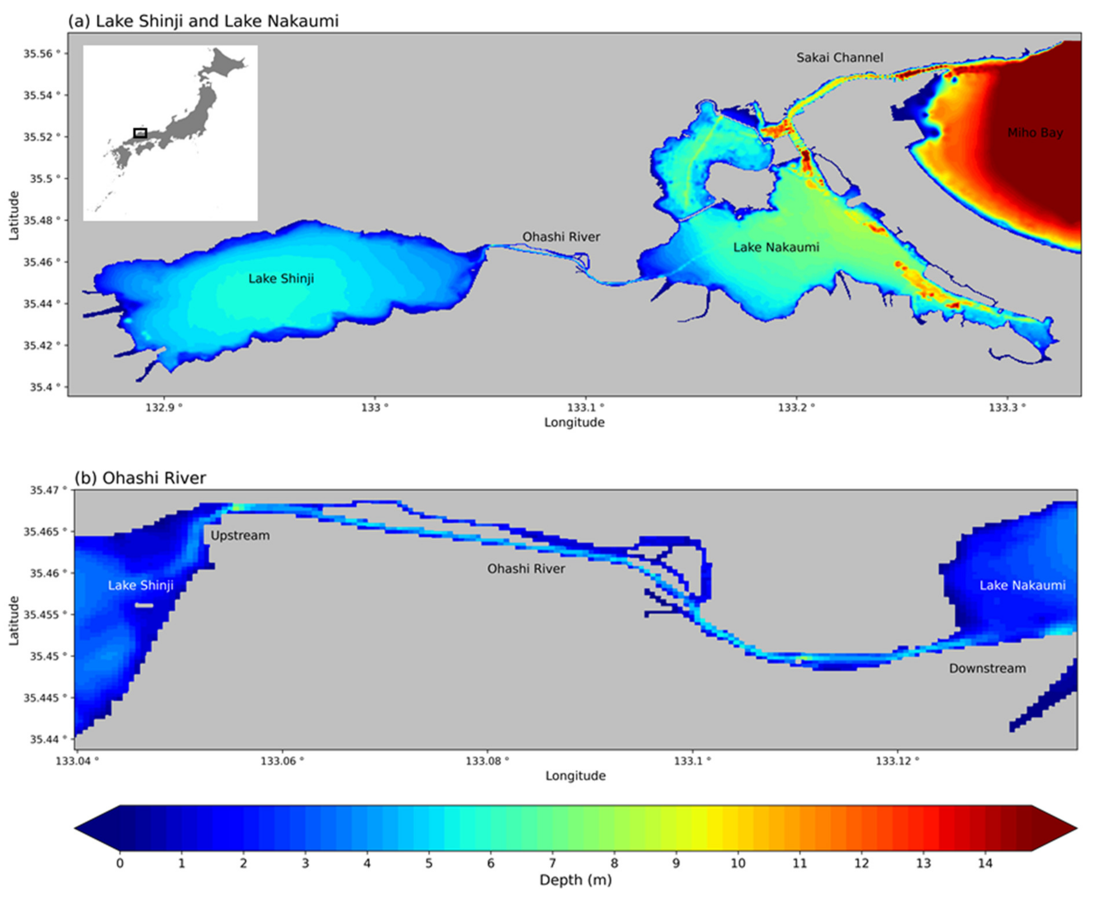
2.1. Study Area

The Ohashi River is a narrow channel that connects two brackish lakes called Lake Shinji (Area: 79.1 km², Average water depth: 4.5 m) and Lake Nakaumi (Area: 86.2 km², Average water depth: 5.4 m) (see Figure 1a). This coupled brackish lake system is a rich fishery resource and a home to filter-feeding bivalves. The area of each lake is ranked seventh and fifth in Japan, but the combined area of the two lakes connected by the Ohashi River, which is about 7 km in length, is the largest brackish lake system in Japan. The salinity of Lake Shinji is relatively low, about one-tenth of the seawater, while Lake Nakaumi has a higher salinity of about one-half of the seawater, and each lake has its unique environment. Lake Shinji has a mesohaline environment, while Lake Nakaumi has a stable two-layered stratified environment with a clear distinction between the surface- and bottom-water salinity. The Ohashi River plays an important role in the circulation process between both lakes and serves as a conveyer belt of both the fresh and saline water. The Ohashi River has a complex shape with meandering and splitting branches of different water depths (see Figure 1b), which makes it very challenging to reproduce the water exchange. The major quantity of freshwater drained into Lake Shinji from the Mount Sentsu watershed (Area: 2070 km²) through the Hii River eventually reaches Lake Nakaumi after passing from Lake Shinji and the Ohashi River. This is the reason the average water transport from upstream of the Ohashi River is approximately equal to the freshwater inflow of the Hii River, while on the other hand, the saline water which intrudes intermittently from the Sea of Japan into Lake Nakaumi through the Sakai Channel intrudes into Lake Shinji along the bottom of Lake Nakaumi and the Ohashi River. As compared to the Pacific side of the Japanese coast, the tidal stirring is the least effective on the Sea of Japan side due to the meager tidal amplitude where the wind and gravity-driven currents are considered the potential mechanism of water exchange.

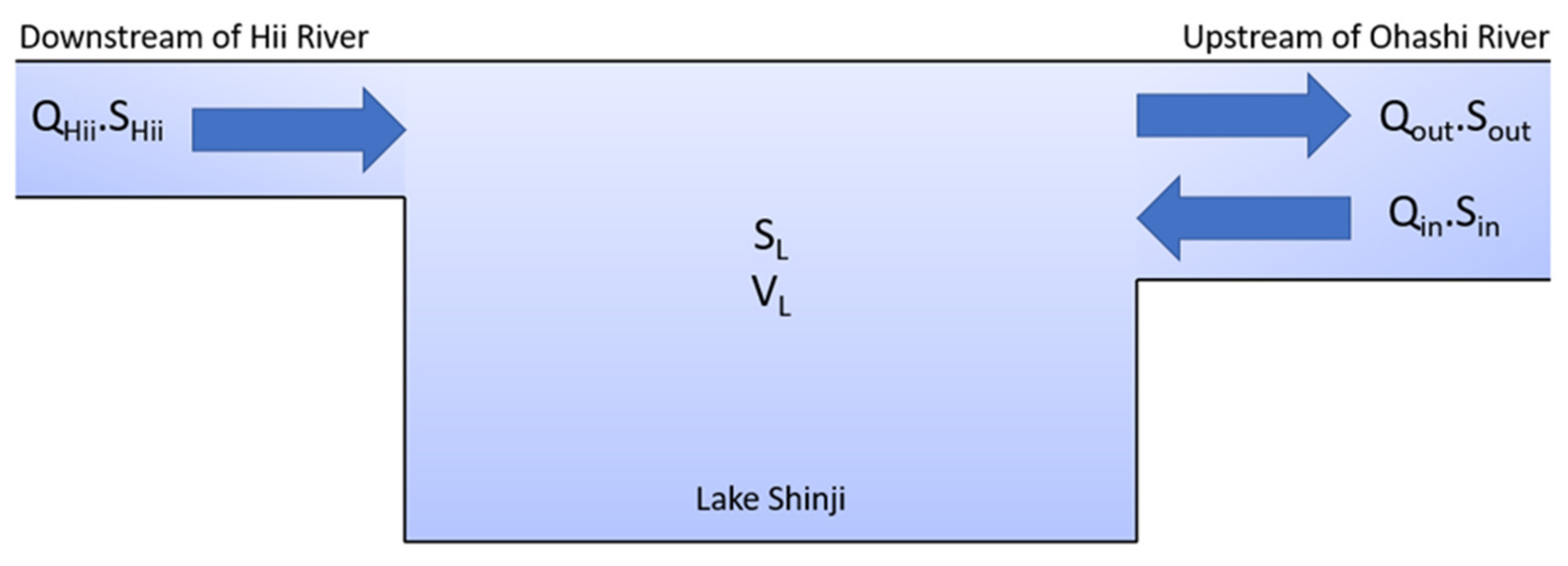
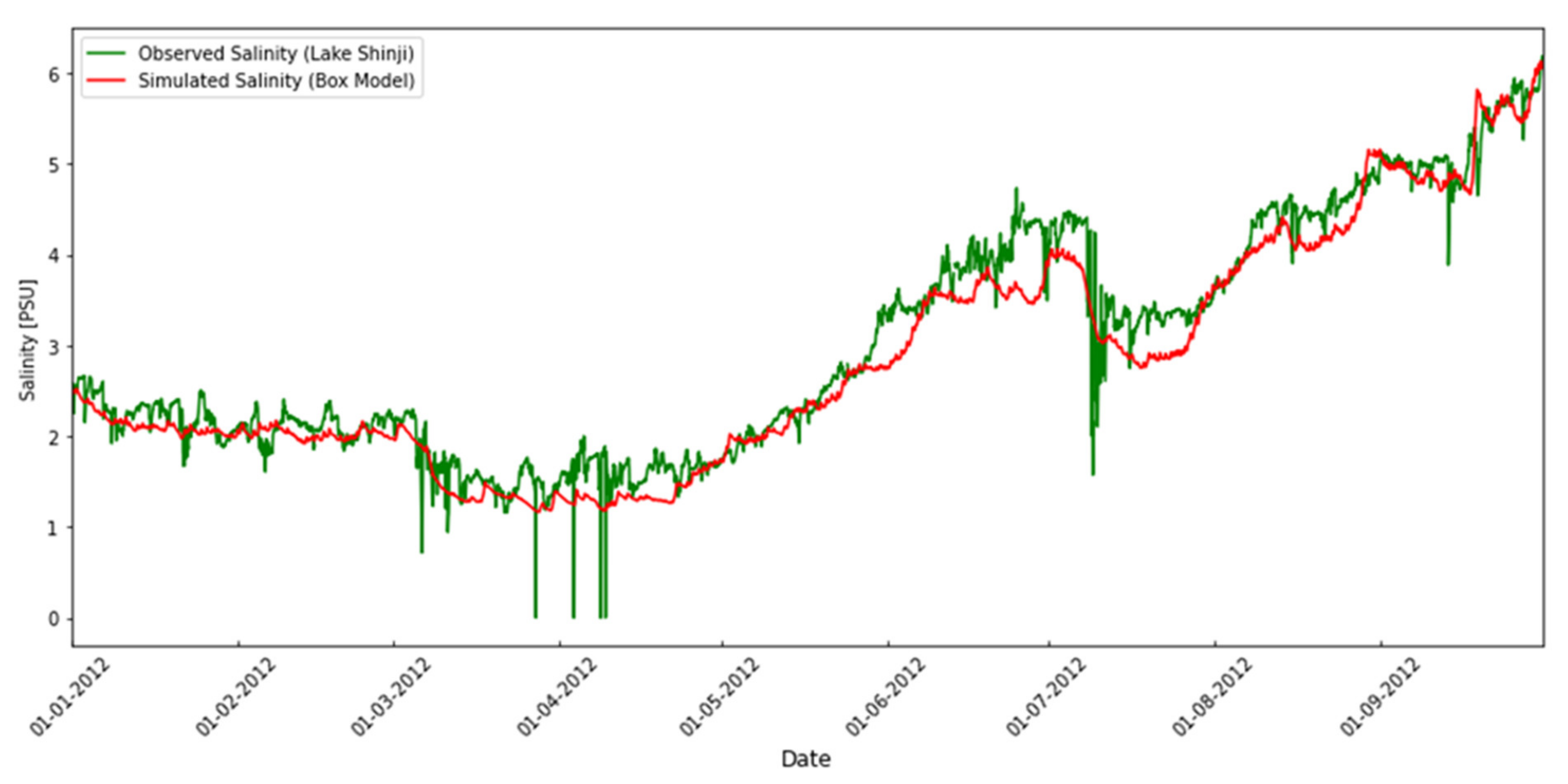
2.2. Reliability of Observed Flowrate of Ohashi River and Its Control Over Salinity Variation of Lake Shinji

The accurate simulation of the flowrate of the Ohashi River was not only important to understand the flow characteristics of the river itself, but it was rudimentary to determine the control of saline water intrusion over the salinity variation of Lake Shinji. To validate the observed flowrates, an indirect approach was adopted, and a box model of the salt budget was developed (see Equations (1) and (2)) for Lake Shinji, which is situated at the upstream end of the Ohashi River. A box model technique is quite common for simulating the average state of the system by considering the mass balance and roughly taking into account the system heterogeneities [11]. As the Ohashi River is the only source of saline water intrusion in Lake Shinji, the overall salinity in Lake Shinji must be controlled by the salt balance at the upstream side of the Ohashi River. If the observed flowrate values, which are the prime inputs of the box model, are reliable it will eventually reproduce the salinity variation in Lake Shinji. The following, in Figure 2, shows all the input parameters utilized in the box model.

Figure 2. Box model for the salt budget of Lake Shinji observed over nine months from the beginning of January 2012 to the end of September 2012.

Figure 2. Box model for the salt budget of Lake Shinji observed over nine months from the beginning of January 2012 to the end of September 2012.

$$\frac{\partial S_L}{\partial t}\times V_L=Q_{Hii}\times S_{Hii}+Q_{in}\times S_{in}-Q_{out}\times S_{out}$$

(1)

$$S_L=S_{LO}+\left(\frac{Q_{Hii}\times S_{Hii}.\Delta t+Q_{in}\times S_{in}\times \Delta t-Q_{out}\times S_{out}\times \Delta t}{V_L}\right)$$

(2)

where

• S_L = Salinity of Lake Shinji.
• S_LO = Initial condition of salinity in Lake Shinji; it was taken from observed data.
• S_Hii = Salinity of Hii River water draining into Lake Shinji; it was assumed as zero.
• S_in = Salinity of saline intruded water from upstream of Ohashi River.
• S_out = Salinity of relatively freshwater going out of Lake Shinji through Ohashi River.
• V_L = Volume of Lake Shinji (m³).
• Q_Hii = Flowrate of Hii River.
• Q_in = Depth integrated flowrate of freshwater going out of Lake Shinji.
• Q_out = Depth integrated flowrate of saline water intruding along the bottom of Ohashi River.
• ∆t = Time Interval between observations (s).

All salinity values are observed in PSU unit while flowrates are measured in cumecs (m³/s).

As observed, the flowrates at the upstream of the Ohashi River were given in the depth-integrated form, while the salinity values were given in layered format. Therefore, to determine the surface and bottom salinities associated with the inflow and outflow, a depth-averaged methodology was adopted.

2.3. Description and Configuration of Hydrodynamic Model

To simulate the hydrodynamics of the Ohashi River, a 3-D non-hydrostatic model called the Ise Bay simulator was used [12]. The model is capable of simulating hydrodynamics as well as ecosystem conditions [13,14,15]. However, for this study, the ecosystem sub-model was switched off and only the hydrodynamics were calculated in a hindcast mode. The hydrodynamic model consists of the sea state equation (Equation (3)), the basic continuity equation (Equation (4)), and the equation of motion (Equations (5)–(7)). To calculate the scalar quantities, such as water temperature and salinity, the model also includes the scalar transport equation (Equations (8) and (9)). The large eddy simulation (LES) model was used to calculate turbulent kinematic viscosity and eddy diffusivity in the horizontal direction [16], while for the vertical direction an improved turbulent diffusion approach analytical model was used, originally developed by Henderson-Sellers [17] and later improved by Nakamura et al., in 1991 [18].

The model domain covers the Ohashi River with both ends as an open boundary, as shown in Figure 3 and Figure 4. The Asakumigawa river was used as the riverine input. The modeling domain is approximately 6.2 km × 3 km in the east–west and north–south directions, respectively. The mesh system has 465 surface water cells for a coarser grid, with a grid size of 200 m, and 22 vertical layers, with a grid size of 50 cm, while for the finer mesh surface the water cells are 6096 in number, with a grid size of 50 m, and the same configuration was adopted for the vertical layers as a coarser grid. The time step diverges from 5 s to 25 s for the coarse resolution. However, the timestep varies from 1 s to 5 s for the fine resolution. Lastly, the water levels and vertical profiles of the water temperature and salinity were provided at both ends of the domains, i.e., upstream and downstream of the Ohashi River (See

Table 1. Configuration of the hydrodynamic model.

Model	Ise Bay Simulator
Simulation Period	Initial Simulation: 1 July 2012 to 31 July 2012 Final Simulation: 1 July 2012 to 30 September 2012
Meshing	Coarser Mesh: Horizontal: 200 m × 200 m (31 × 15 grid points) Vertical: 22 layers (−8.0 m to 1.0 m) Finer Mesh: Horizontal: 50 m × 50 m (127 × 48 grid points) Vertical: 22 layers (−8.0 m to 1.0 m)
Turbulence Model (Horizontal)	Sub grid-scale model (SGS)
Turbulence Model (Vertical)	Nakamura Model (Improved Henderson-Sellers Model)
Input data	Water Level: Hourly Tides at both ends of Ohashi River. Open Boundary Conditions: Hourly water quality profile observed at upstream and downstream of Ohashi River. River Discharge: Observed RD of Asakumigawa. Weather Data: Air Temperature, Solar Radiation, Wind Velocity, Wind Direction, and Precipitation (Observed at Matsue weather station).
Land Water Interface Conditions	Coefficient of Friction (River Bed): 0.0026 Coefficient of Friction (Vertical River Wall): 0.00

and

Table 2. Model input conditions with corresponding parameters and sources responsible for its provision.

Model Input Conditions	Parameters	Source
Initial Conditions	Water Temperature, Salinity, Elevation	Arbitrary Value
Surface Conditions	Air Temperature, Solar Radiation, Wind Components, Rainfall, Surface Pressure, Vapor Pressure	JMA
Open Boundary Conditions	Water Temperature, Salinity	MLIT
Riverine Conditions	River Discharge, Water Temperature, Salinity	MLIT

).

$$\rho =\rho \left(T,S\right)$$

(3)

$$\frac{\partial u}{\partial x}+\frac{\partial v}{\partial y}+\frac{\partial w}{\partial z}=0$$

(4)

$$\begin{array}{l}\frac{\partial u}{\partial t}=-\frac{\partial uu}{\partial x}-\frac{\partial vu}{\partial y}-\frac{\partial wu}{\partial z}+f_{0}v-\frac{1}{{\rho }_0}\frac{\partial p}{\partial x}-g\frac{\partial \eta }{\partial x}-\frac{1}{{\rho }_0}\frac{\partial }{\partial x}\left(p_a+{{\displaystyle \int }}_z^{\eta }{\rho }^{\prime }gdz\right)\\ \hspace{1em}\hspace{1em}\hspace{1em}\hspace{1em}\hspace{1em}\hspace{1em}+\frac{\partial }{\partial x}\left(2{\nu }_h\frac{\partial u}{\partial x}\right)+\frac{\partial }{\partial y}\left\{{\nu }_h\left(\frac{\partial u}{\partial y}+\frac{\partial v}{\partial x}\right)\right\}+\frac{\partial }{\partial z}\left\{{\nu }_v\left(\frac{\partial u}{\partial z}+\frac{\partial w}{\partial x}\right)\right\}\end{array}$$

(5)

$$\begin{array}{l}\frac{\partial v}{\partial t}=-\frac{\partial uv}{\partial x}-\frac{\partial vv}{\partial y}-\frac{\partial wv}{\partial z}-f_{0}u-\frac{1}{{\rho }_0}\frac{\partial p}{\partial y}-g\frac{\partial \eta }{\partial y}-\frac{1}{{\rho }_0}\frac{\partial }{\partial y}\left(p_a+{{\displaystyle \int }}_z^{\eta }{\rho }^{\prime }gdz\right)\\ \hspace{1em}\hspace{1em}\hspace{1em}\hspace{1em}\hspace{1em}\hspace{1em}+\frac{\partial }{\partial x}\left\{{\nu }_h\left(\frac{\partial v}{\partial x}+\frac{\partial u}{\partial y}\right)\right\}+\frac{\partial }{\partial y}\left(2{\nu }_h\frac{\partial v}{\partial y}\right)+\frac{\partial }{\partial z}\left\{{\nu }_v\left(\frac{\partial v}{\partial z}+\frac{\partial w}{\partial y}\right)\right\}\end{array}$$

(6)

$$\begin{array}{l}\frac{\partial w}{\partial t}=-\frac{\partial uw}{\partial x}-\frac{\partial vw}{\partial y}-\frac{\partial ww}{\partial z}-\frac{1}{{\rho }_0}\frac{\partial p}{\partial z}-\frac{{\rho }^{\prime }}{{\rho }_0}g+\frac{\partial }{\partial x}\left\{{\nu }_h\left(\frac{\partial w}{\partial x}+\frac{\partial u}{\partial z}\right)\right\}\\ \hspace{1em}\hspace{1em}\hspace{1em}\hspace{1em}\hspace{1em}\hspace{1em}+\frac{\partial }{\partial y}\left\{{\nu }_h\left(\frac{\partial w}{\partial y}+\frac{\partial v}{\partial z}\right)\right\}+\frac{\partial }{\partial z}\left(2{\nu }_v\frac{\partial w}{\partial z}\right)\end{array}$$

(7)

$$\frac{\partial T}{\partial t}=-\frac{\partial uT}{\partial x}-\frac{\partial vT}{\partial y}-\frac{\partial wT}{\partial z}+\frac{\partial }{\partial x}\left(K_h\frac{\partial T}{\partial x}\right)+\frac{\partial }{\partial y}\left(K_h\frac{\partial T}{\partial y}\right)+\frac{\partial }{\partial z}\left(K_v\frac{\partial T}{\partial z}\right)+\frac{1}{\rho c_p}\frac{\partial Q_s}{\partial z}$$

(8)

$$\frac{\partial C}{\partial t}=-\frac{\partial uC}{\partial x}-\frac{\partial vC}{\partial y}-\frac{\partial wC}{\partial z}+\frac{\partial }{\partial x}\left(K_h\frac{\partial C}{\partial x}\right)+\frac{\partial }{\partial y}\left(K_h\frac{\partial C}{\partial y}\right)+\frac{\partial }{\partial z}\left(K_v\frac{\partial C}{\partial z}\right)+S_C$$

(9)

where $u$, $v$, and $w$. are the velocity components; $\eta$ is the free water surface elevation; $p_d=p$ and $p_a$ are dynamic and atmospheric pressures; $\rho$ and ${\rho }_0$ are in situ and standard densities, while density deviation is expressed as ${\rho }^{\prime }=\rho -{\rho }_0$; $g$ is gravitational acceleration; $f_0$ is the Coriolis parameter; ${\nu }_h$ and ${\nu }_v$ are the horizontal and vertical kinematic turbulent viscosities; $K_h$ and $K_v$ are the horizontal and vertical eddy diffusivities; $c_p$ represents the specific heat capacity of water; $Q_s$ is the solar radiation; $C$ is the water quality scalar quantity (salinity); and $S_C$ is the external generation rate.

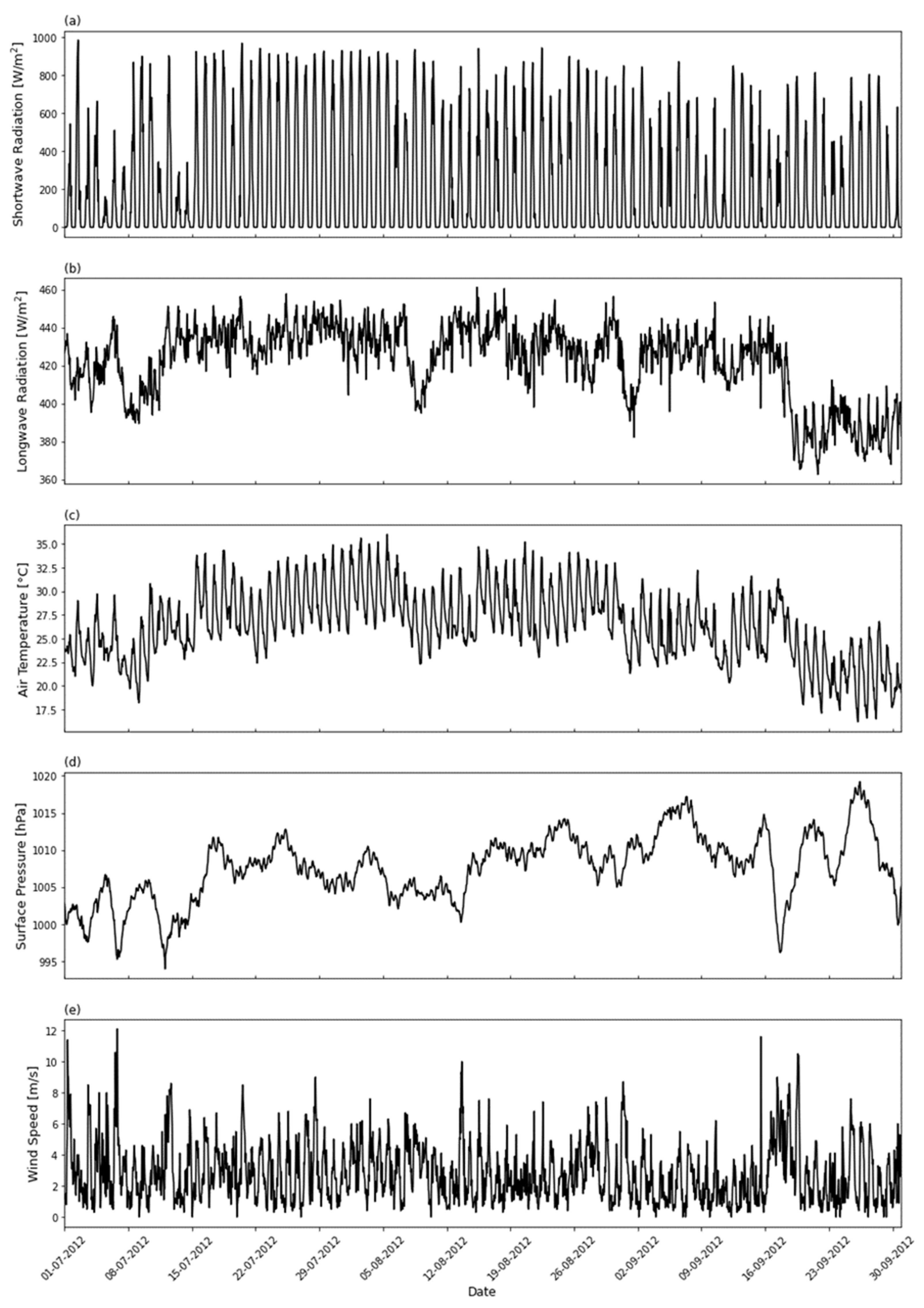
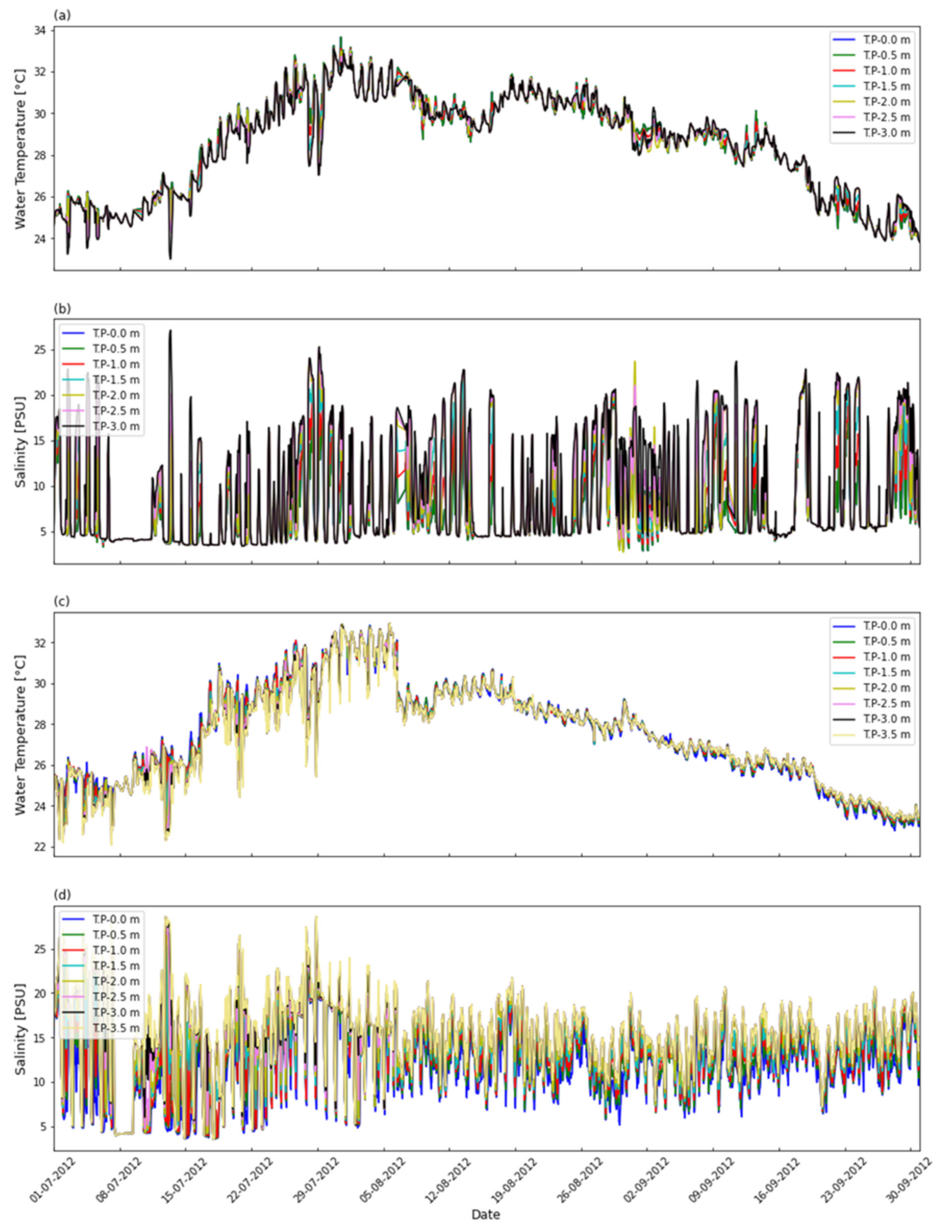
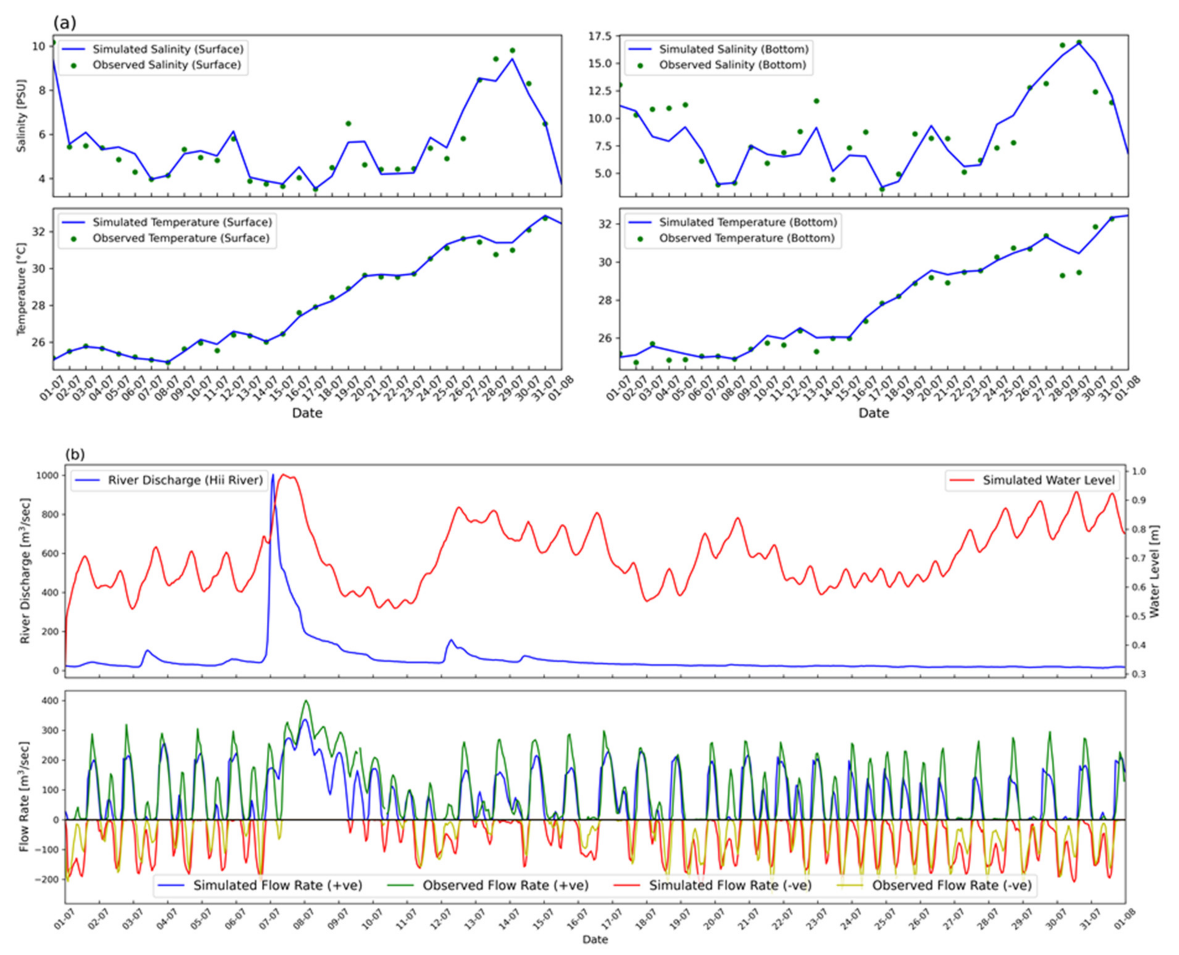
2.4. Initial and Boundary Conditions for Hydrodynamic Simulations

The hydrodynamic model requires several input parameters as the initial and boundary conditions to initiate the simulation. For the initial conditions, the model input parameters are water temperature, salinity, and water elevation, i.e., usually an arbitrary value taken from the observed data. Furthermore, for the riverine input, the model takes the actual river discharge with the corresponding river water temperature and salinity. Air temperature, solar radiation, wind components, rainfall, atmospheric pressure, and vapor pressure are the surface-input weather conditions. The following Figure 5, shows the time series of the observed weather conditions at the Matsue weather station, taken from the Japan Meteorological Agency (JMA). For the usual open boundary conditions, the model takes several input parameters for the entire water column, including the hydrodynamic and ecosystem parameters. However, for the subject study, the water temperature and salinity profile were the only parameters utilized as the input open-boundary conditions at both ends of Ohashi River and were taken from the observed data. The Ministry of Land, Infrastructure, Transport, and Tourism (MLIT) records these observations on an hourly basis. The following Figure 6 shows the time series (2012-07-01 to 2012-09-30) of the water temperature and salinity for different water depths starting from the surface (T.P −0.0 m) to the bottom (T.P −3.0 m) and (T.P −3.5 m). The aforementioned Table 2 summarizes the input parameters required to execute the hydrodynamic simulations with the corresponding sources.

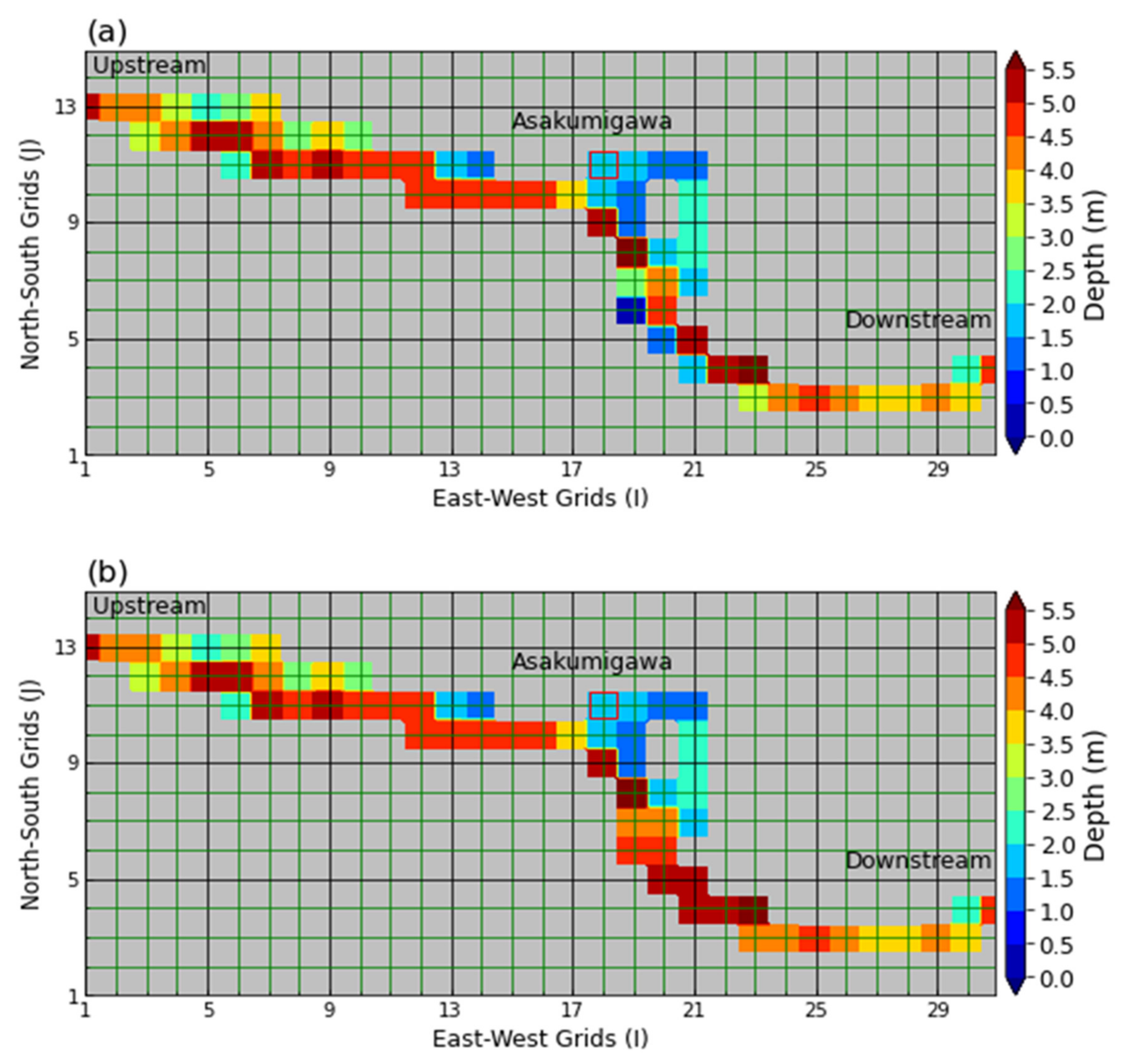
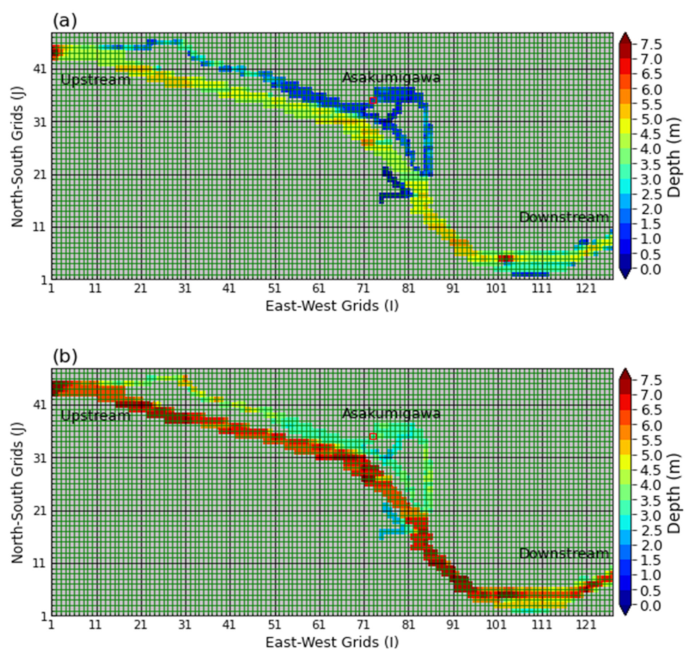
2.5. Experiments Design

Table 3. Experimental cases of hydrodynamic simulations for coarser and finer mesh grid bathymetric maps.

Case	Meshing		Average Water Depth (m)	Area (m2)	Volume (m3)
	I, J, K (#)	Size (dx, dy, dz) (m)
1	31, 15, 22	200, 200, 0.50	3.46	2,520,000	8,726,000
2	31, 15, 22	200, 200, 0.50	3.69	2,520,000	9,301,200
3	127, 48, 22	50, 50, 0.50	3.33	1,570,000	5,236,925
4	127, 48, 22	50, 50, 0.50	5.32	1,570,000	8,348,975

summarizes the cases tested to obtain the most appropriate mesh configuration to reproduce the flow conditions. The first column of Table 3 shows the number of cases tested while the second column presents the number of grids in the X, Y, and Z directions. The 3rd column shows the grid size in all three directions, while the 4th and 5th columns are showing the actual river area and river volume taking part in the hydrodynamic simulation. For case 1 (hereafter the default case for the coarser meshing), the coarse-resolution 200 m × 200 m mesh was used with a river area of 2,520,000 m² and a volume of 8,726,000 m³. In case 2, the depth modifications were made to the grid numbers (19, 6), (19, 7), (20, 5), (21, 4), and (23, 3). The idea of the depth modification was pretty simple as those depths were altered which were shallower than the adjacent depths and seemed to be hindering the flowrate. The depth of grid numbers (19, 6) and (19, 7) was very shallow, and it was in the range of 0.0–3.0 m, and after modifications, the modified grids were in the depth range of 4.0–5.0 m. The depth of grid numbers (20, 5) and (21, 4) was in the range of 1.0–2.0 m, and after modifications, the modified grids were in the depth range of 5.0–5.5 m. The depth modifications in the 2nd case increased the overall river volume, with reference to the default river volume, by 6.59%. The following Figure 3 graphically represents the difference in two cases of coarser mesh configuration. The upper panel (a) is the default case while panel (b) is the 2nd case. There was no widening of river width considered for the coarser mesh, and the width was kept on a relatively representative side. In the subsequent cases, a more detailed meshing was used. Numerous simulations were conducted with the default fine-resolution mesh having a river area of 1,410,000 m² and a volume of 3,785,125 m³. The default fine-resolution mesh and the alteration to its width and depth were inadequate to reproduce the flowrates. Therefore, the default fine-resolution mesh was altered, and a relatively wider and deeper default fine-mesh resolution was created. In the case of the new default finer mesh, the river widening was carried out and additional grids were added to increase the width of the river. The altered default fine-resolution mesh was utilized in case 3, and it was referred to as the default case for the fine-resolution mesh. For case 3 (hereafter the default case for the finer meshing), the fine-resolution 50 m × 50 m mesh was used with a river area of 1,570,000 m² and a volume of 5,236,925 m³. For the detailed mesh cases, the Ohashi River was split into two branches in the middle of the domain. The first branch was referred to as the northern branch and it was shallower in depth, while the second branch, i.e., the relatively deeper one, was referred to as the southern branch. In case 4, the depth modifications were made to the entire river area by adding 2.0 m to all depths. The depth modifications in the 4th and last case increased the overall river volume by 59.43%, with reference to the fine-mesh default river volume, which made its volume closer to the default coarse case. The following Figure 4 graphically represents the difference in the two cases of finer mesh configuration. The upper panel (a) is the default case while panel (b) is the fourth and last case.

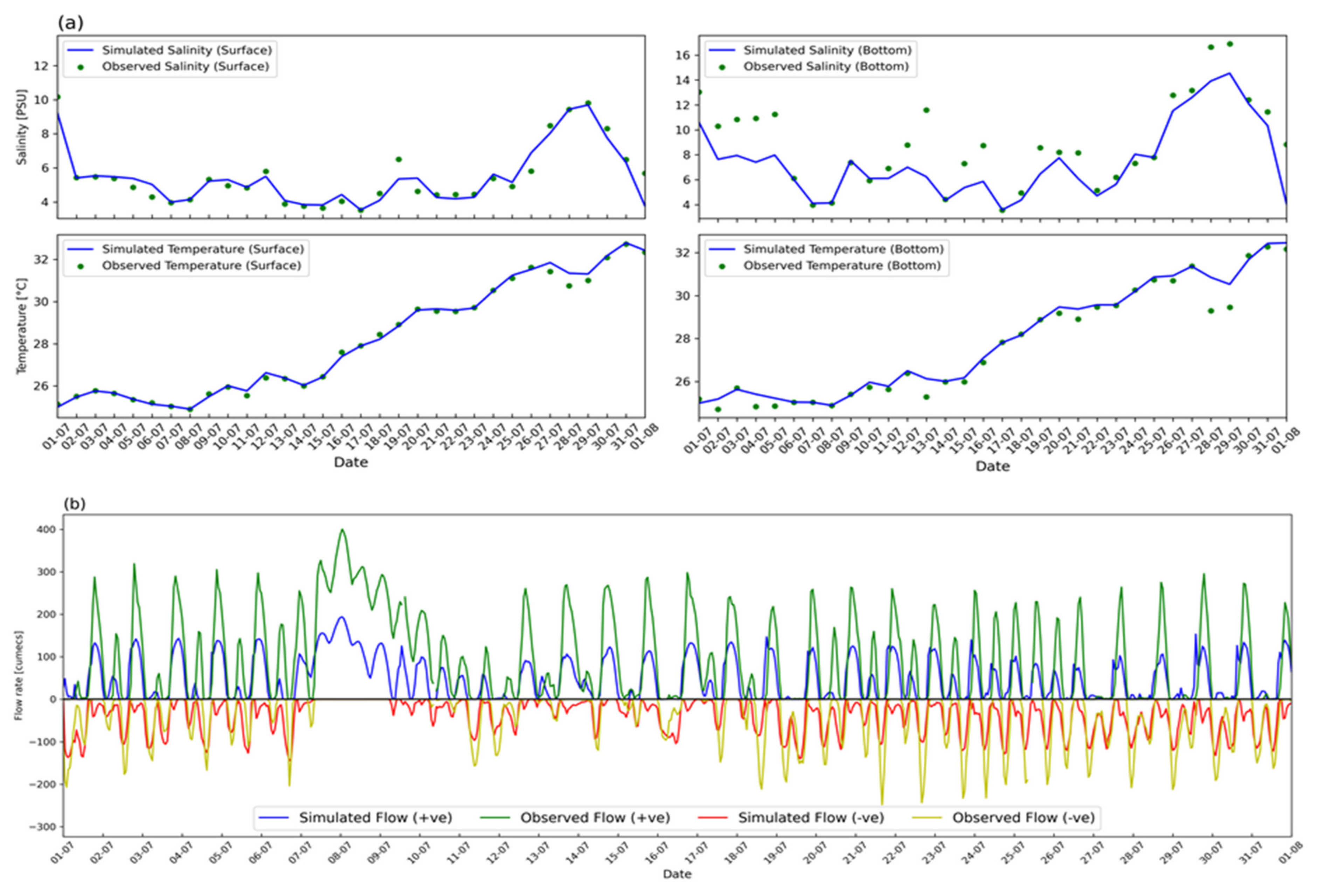
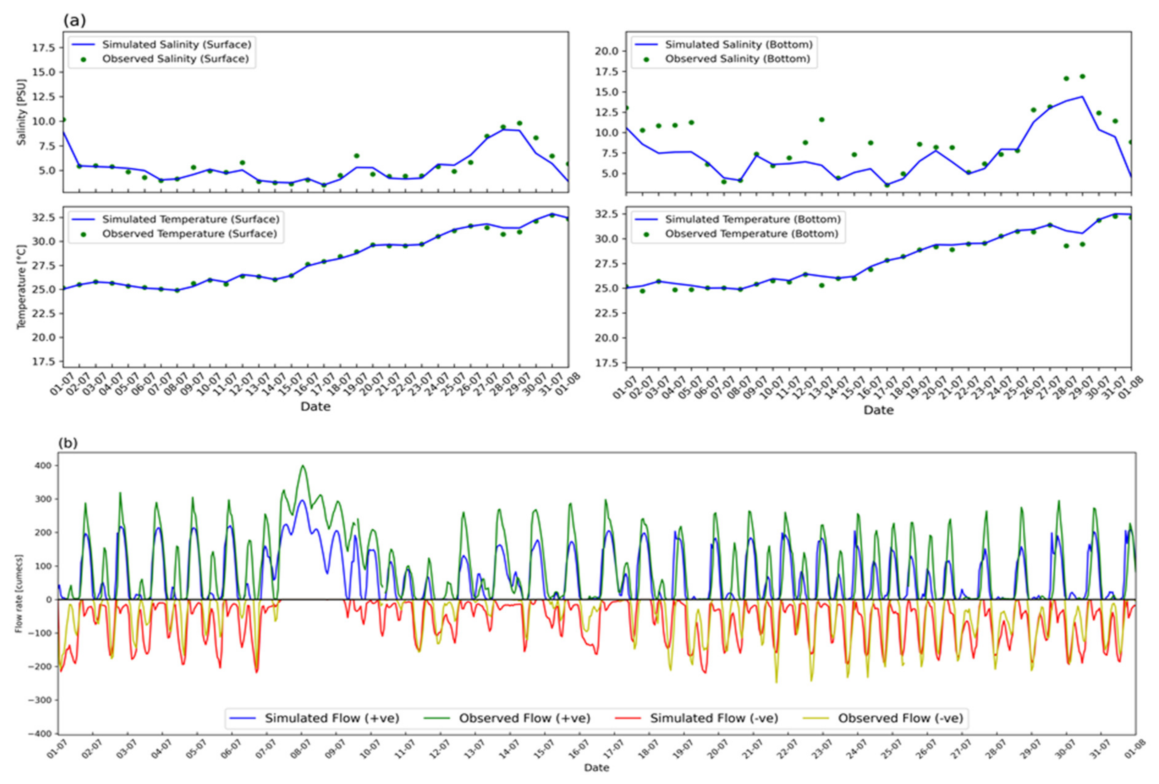
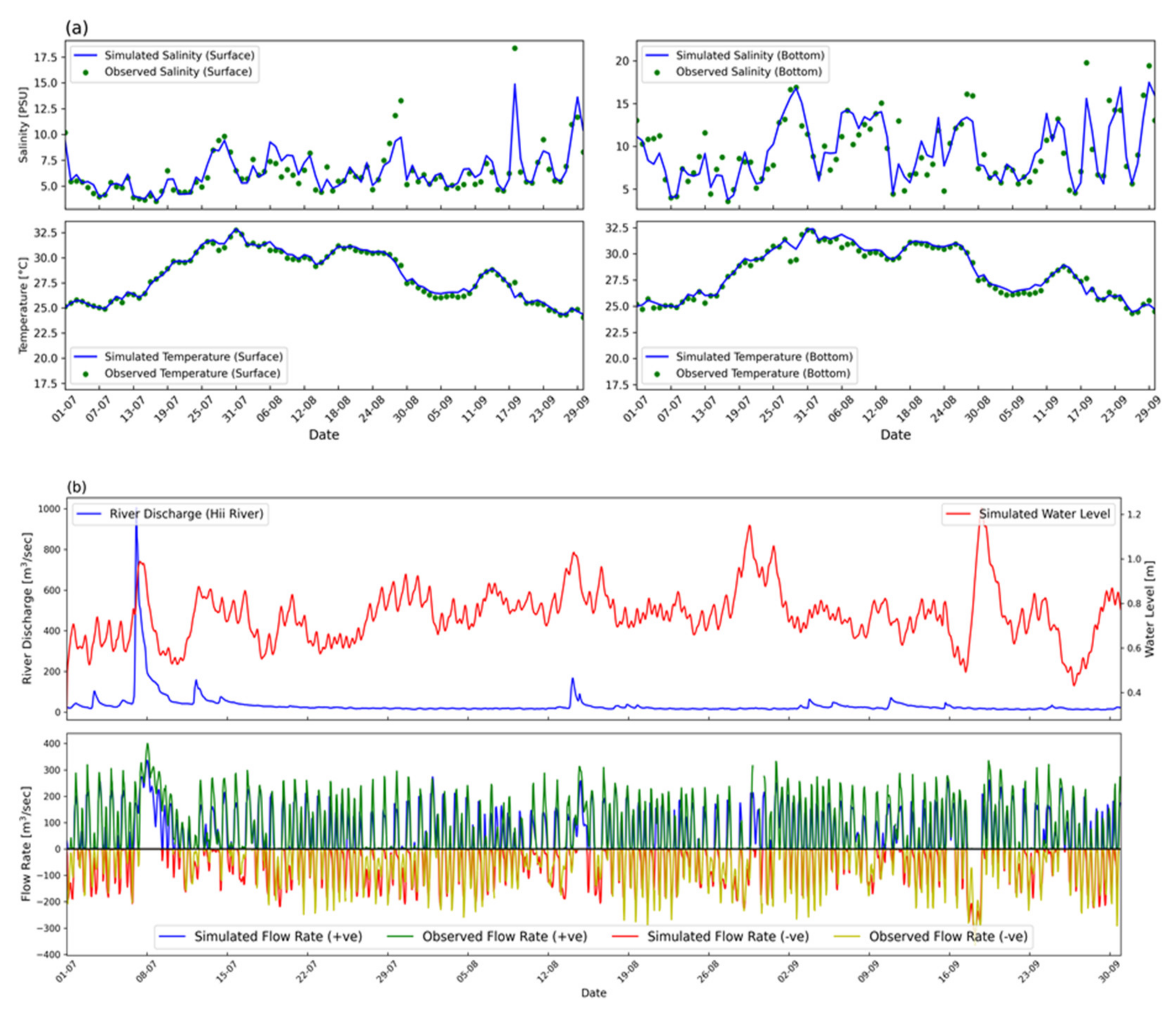
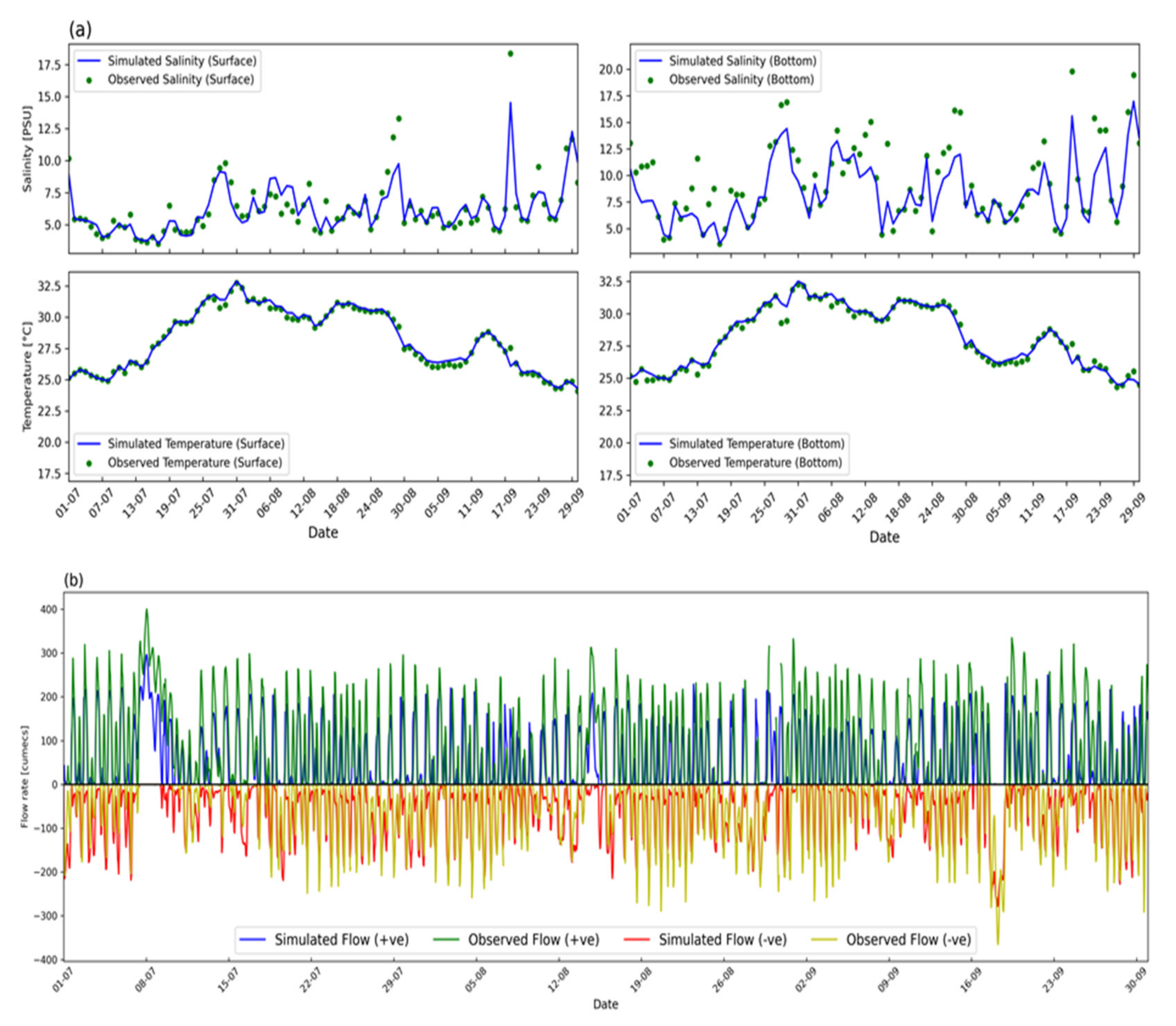
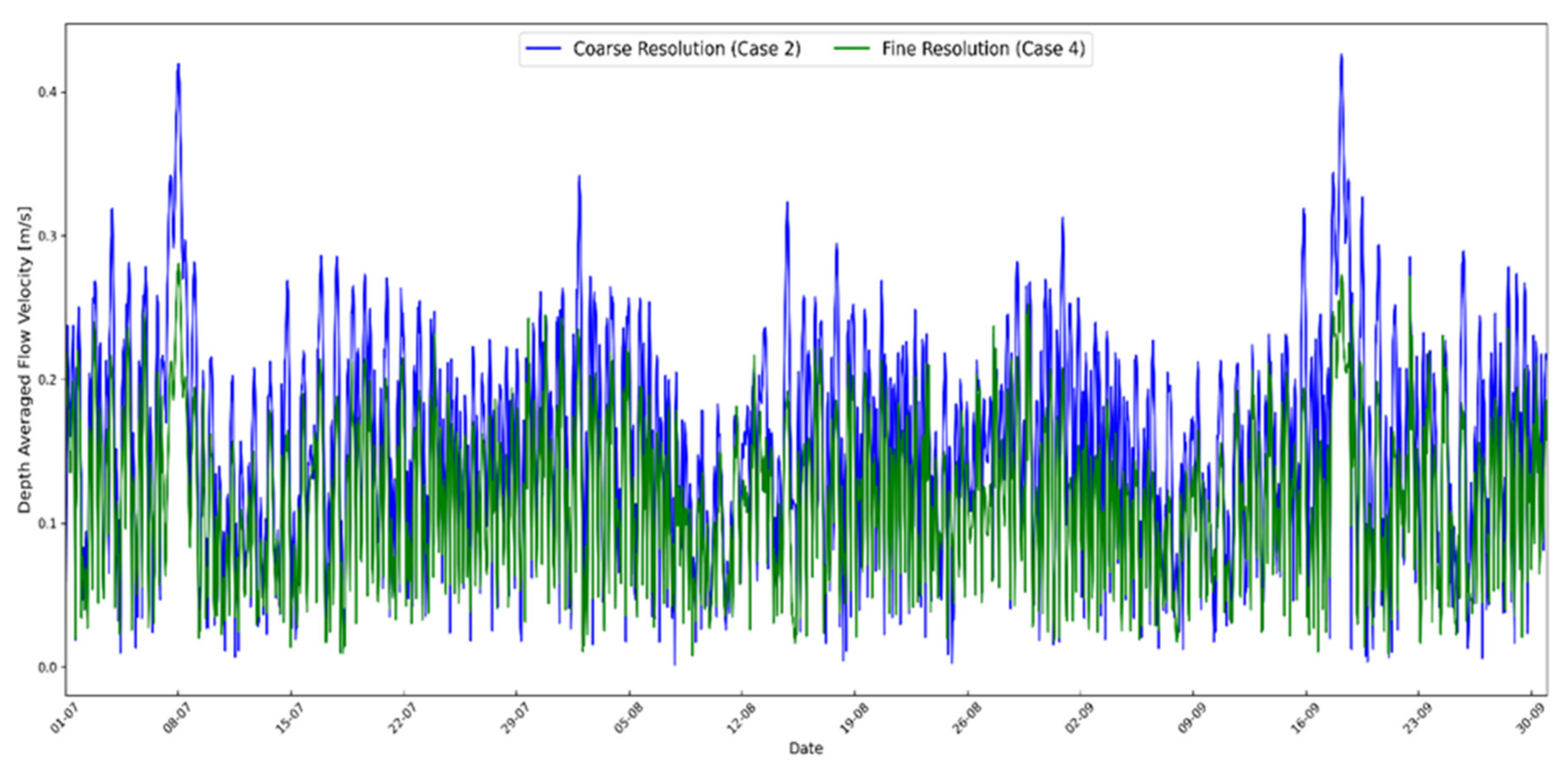
3. Results and Discussions

3.1. Reliability of Observed Flowrate

As described earlier, the box model was formulated to assess the accuracy of the observed flowrates. For the first trial, the topmost-layer salinity was assumed as the surface salinity (S_out) while the bottom-layer salinity was considered as S_in. Similarly, for the subsequent trials, the average of the different layers was computed to obtain the surface- and bottom-water salinity. The most accurate trial was the one in which the surface salinity was calculated by taking an average of the three surface layers (S_0m, S_0.5m, and S_1m), while the bottom salinity was taken by the average of the bottom three layers (S_2m, S_2.5m and S_3m), while the depth difference in each layer was only 50 cm. The following Figure 7 graphically represents the range of the surface- and bottom-water salinity. The following Figure 8 demonstrate the time-series comparison of the observed salinity of Lake Shinji and the simulated salinity variation of Lake Shinji by the box model. Overall, the box model performed pretty well and reproduced the lake salinity variation and indirectly gave evidence of highly reliable, observed flowrates.

3.2. Numerical Simulations

The unique geographical and bathymetric conditions of the Ohashi River play an important role in the water-exchange process of the coupled Lake Shinji and Lake Nakaumi lagoon system. The core emphasis of this study was given to the reproducibility of the water-exchange characteristics of the Ohashi River. The top panel in Figure 9 shows the comparison of the salinity and water temperature at the upstream surface and bottom layers of the Ohashi River. The simulation results of the coarser mesh configuration revealed a fair reproducibility of the salinity and water temperature under all the cases, as shown in Figure 9 and Figure 10. However, the underestimation of the water transport was encountered in the default case 1, which was further improved in case 2 by altering the mesh files. Depth modifications to the mesh files did not make any significant difference to the salinity and water-temperature time series; however, it did make a significant improvement to the flowrate. There was no river widening in the case of the coarse-mesh simulation; that is why increasing the depth of a few grids removed the hindrance of flow by removing the bottom sills. In the past, Nakata et al., 2000, also calculated the flowrate of the Ohashi River to explain the water-exchange mechanism between both lakes; however, the simulation results were not compared with the observed values [19]. The authors somehow indicated the underestimation of the saline water intrusion from Lake Nakaumi to Lake Shinji by comparing the salinity result of Lake Shinji as the model simulation showed lower salinity values as compared to the observed values. In comparison with the previous study by Nakata et al., 2000, where the flowrate varied between a range of 50 m³/s to 200 m³/s in July 1995, the present study indicated a relatively higher flowrate range of 200 m³/s to 400 m³/s in July 2012.

The following

Table 4. Performance evaluation of flowrate simulations under different bathymetric conditions. A regression comparison was made for the initial simulation period covering July 2012.

Case	R2		RMSE
	Westward Flow	Eastward Flow	Westward Flow	Eastward Flow
1	0.65	0.58	75.31	36.49
2	0.72	0.61	56.40	43.43
3	0.61	0.55	96.64	40.16
4	0.64	0.59	78.03	39.63

summarises the performance evaluation by two performance indicators, the coefficient of determination (R²) and the root mean square error (RMSE). The following Equations (10) and (11) were used to calculate the performance indicators. The regression comparison was made for all the initial cases conducted for one month. Case 1 resulted in a higher RMSE value for the positive flow direction (eastward) and underestimated the flow from Lake Shinji to Lake Nakaumi. In case 2, not only the R² but also the RMSE improved for the positive flow direction; however, the RMSE slightly worsened for the negative flowrate conditions (westward). As the focus of this study was to determine the flowrate characteristics, it was essential to give equal weightage to both flow directions. Because of this reason, case 2 was adopted as the best case for the coarse-resolution simulation; despite the slight deterioration of the negative flowrate, the positive flowrate significantly improved.

The default fine-resolution case 3 resulted in a worse performance; the R² was found to be the least among all the cases, while the RMSE for the positive flowrate was found to be the highest amongst all the cases. The depth modifications in case 4 significantly improved the performance of both simulations with reference to the default case; however, in comparison with the coarse-resolution best case, the performance of the fine resolution was still bad. Some additional trials were also conducted in the fine-resolution cases by reducing the bottom friction coefficient to zero to increase the flowrate by reducing the flow resistance; however, it did not make any improvement and turned out to be the same.

$$R^2=\frac{\sum {\left(\widehat{y}-\overline{y}\right)}^2}{\sum {\left(y_i-\overline{y}\right)}^2}$$

(10)

where $\widehat{y}$ are predicted values while $y_i$ are observed values and $\overline{y}$ is the mean of observation.

$$RMSE=\sqrt{\frac{1}{N}{\displaystyle \sum }_{i=1}^N{\left(\widehat{y}-y_i\right)}^2}$$

(11)

where $\widehat{y}$ are predicted values while $y_i$ are observed values and N is the sample size.

It was interesting to see the overall good performance of both mesh configurations in simulating the water temperature and salinity. Despite the bad performance of the fine-mesh files in the flowrate simulations, the water temperature and salinity in the surface and bottom layers were in good agreement with the observations, as shown in subplot (a) of Figure 11 and Figure 12. As the Ohashi River connects two brackish lakes and serves as a conveyer belt of fresh and saline water, it was thus essential to only achieve a certain accuracy for the water temperature and salinity but also for the quantity of transferred water as well. In this study, the coarse-mesh configuration showed its superiority over the fine-mesh grid in terms of all the simulated parameters. The coarse-mesh configuration was also found to be less computationally expensive, and the simulations were pretty fast as compared to the fine-mesh configuration.

The performance evaluation was conducted for the optimum bathymetric conditions achieved through the initial simulation trials (case 1 to case 4). A regression comparison was made for the final optimum simulations (case 2 and case 4) from the beginning of July to the end of September 2012. The simulation duration was extended from one month to three months in order to validate the simulations.

Table 5. Performance evaluation of flowrate simulations under optimum bathymetric conditions achieved through initial simulation trials. A regression comparison was made for the final optimum simulation from the beginning of July to the end of September 2012.

Case	R2		RMSE
	Westward Flow	Eastward Flow	Westward Flow	Eastward Flow
2	0.66	0.66	56.73	42.05
4	0.50	0.60	78.86	43.09

summarises the performance indicators, and once again the coarse-mesh configuration outperformed the fine-mesh configuration. An R² of 0.66 was achieved in case 2 for both the positive and the negative flow directions, while an R² of 0.51 and 0.56 was obtained for both the flow directions of case 4, respectively. Even though case 2 performed better than case 4 for both flow directions, the RMSE for the negative flow direction was not so different in both cases. In case 4, the RMSE of the positive flow direction was much higher as compared to that of case 2. A time-series comparison was also made for both of the extended duration cases, as shown in Figure 13 and Figure 14.

To understand the difference in the coarse- and fine-resolution simulations, a square root correlation between the simulated flow velocity and the difference between the end water levels was determined. It was revealed that the coarse-resolution simulations were able to produce higher water flux coefficients as compared to the fine-resolution simulations, as shown in Table 6. This square root correlation was derived from the hydraulic theory and it demonstrates the commonly occurring phenomenon in straits where hydraulic currents in the straits are primarily controlled by pressure difference due to differential tidal movements at the end of the straits [20]. In the past, this square root correlation was effectively used to predict the flow through the Cape Cod Canal [21], and for the subject study area in this research, i.e., the Ohashi River [8]. The following Equation (12) mathematically represents the square root correlation between the two parameters.

$$u^2=K^2 \left(│\Delta h\pm c│\right)$$

(12)

where

• u = Westward flow velocity (m/s)
• K = Water flux coefficient (m^1/2/sec⁻¹).
• ∆h = Water level difference between the upstream and downstream of Ohashi River (m).
• c = Regression equation constant.

Previously, Ishitobi et al., 1999 [8], conducted the field observations for both the flow velocity and the water level and calculated the square root calculation based on observed values. The values for the water flux coefficient (K) were in the range of 1.21 to 1.72 m^1/2/s⁻¹; it was higher than the present study for both the fine- and the coarse-resolution simulations, as shown in Table 6. The underlying reasons were the different bathymetric conditions, the cross-sectional areas, and the flow velocity. As in the previous study, a relatively smaller cross-sectional area (A = 470.8 m²) was used as compared to the present study’s cross-sectional area for both the coarse- and the fine-resolution simulations (A = 826 m² and A = 924 m²). However, the combination of the water flux coefficient and the cross-sectional area (K.A) was not so different. As for the previous study, it was in the range of 569.66 to 809.77. The present study’s final accurate coarse-resolution case 2 value also gave the comparable value of 636.02 for the K.A combination. The present study’s results were also compared with another previous study in which the authors determined the square root correlation of the Ohashi River through numerical simulation and calculated the water flux coefficient value of 0.90 m^1/2/s⁻¹ [22]; that value is relatively comparable to the present study.

Table 6. Relationship between simulated upstream flow velocity and the difference between simulated water level at the ends of Ohashi River.

Case	Regression Equation	K.A
1	u2 = 0.532(∆h + c)	437.25
2	u2 = 0.772(∆h + c)	636.02
3	u2 = 0.372(∆h + c)	341.88
4	u2 = 0.492(∆h + c)	452.76

Table 6. Relationship between simulated upstream flow velocity and the difference between simulated water level at the ends of Ohashi River.

Case	Regression Equation	K.A
1	u2 = 0.532(∆h + c)	437.25
2	u2 = 0.772(∆h + c)	636.02
3	u2 = 0.372(∆h + c)	341.88
4	u2 = 0.492(∆h + c)	452.76

Furthermore, the disparity between the case 2 and case 4 simulations was also found and the depth average flow velocity was calculated and further compared. It was found that the overall depth-averaged flow velocity was higher in case 2 as compared to case 4 (see Figure 15). The lower velocity range, which is related to saline water intrusion, is somehow consistent in both simulation cases; however, the peaks of the velocities that are coincident with the positive flow direction are underestimated in case 4. This might be the main reason why a much lower positive flowrate was yielded in case 4 as compared to case 2. In a numerical simulation using the structural grid system, which is espoused in this study, the following two approaches are generally adopted when long and narrow topography, such as a river and a channel, are under consideration. Firstly, if the shape of the water body does not match the set direction of the structural grid, such as if the river channel crosses the grid system diagonally, the channel will be represented as a jagged shape causing structural resistance. In addition, the flow path distance becomes longer than it actually is, and the water surface gradient becomes milder. As a result, the flow velocity is underestimated. If the reproduction of flow velocity is the priority, adjusting the shape resistance and water surface gradient by changing the grid arrangement or reducing the number of grids to reduce the degree of sinuosity are usually considered. However, this has the disadvantage that the topography represented by the grid will be visually different from the actual topography. Initially, a few simulations were conducted using a straightened river map with a relatively lesser meander stretch, and it was found that the flow velocity increased two-fold. The straightened-mesh water flux coefficient was also calculated, and it was found to be higher than in previous studies as well as being the best case 2 of the present study. As the prime importance was given to flowrate simulation in this study, the second approach was found to be more appropriate, in which the change of water depth and the cross-sectional area was adopted to compensate for the underestimation of the flow velocity. All four cases presented in this study represent the second approach of bathymetric modifications. The second approach underestimated the flow velocity and, according to Ishitobi et al., 1999, a typical maximum velocity for the Ohashi River at ebb tide was around 0.6 m/s, but it was around 0.3 m/s in the present study. This difference causes up to a 3-h time lag for water mass to pass through the Ohashi River, which in principle should affect the temporal variations of the water temperature and salinity. Fortunately, as the typical time scale for water temperature and salinity fluctuations in the Ohashi River is a few days (e.g., Figure 13), a 3-h time lag did not cause any problems. As our priority was reproducing flowrate, not flow velocity, the authors considered that choosing the coarse-mesh system was a reasonable option to conduct a numerical calculation of the Ohashi River. In general, the riverbed has a more complex topography than the seabed or lake bottom. Therefore, when the topography is gridded at the same time as that of seas and lakes, the complex topography of the riverbed often cannot be adequately represented due to the limitation of spatial resolution. Therefore, to obtain optimal calculation results for the flowrate, it is inadequate to spatially interpolate the measured bathymetry, but it is required to appropriately adjust the gridded bathymetry and vertical cross-sectional area of each grid.

4. Conclusions

Accurate bathymetric conditions are vital to reproduce the hydrodynamic conditions. However, most of the time accurate and detailed bathymetric data are not readily available because of difficult observations on a larger scale. In such cases, a few observations were interpolated and extrapolated to generate detailed bathymetric maps. In this study, a comparison was made between such conditions; at first, a simplified bathymetric map was used to determine the flow characteristics of a river, and later a detailed bathymetric map was utilized to simulate the same parameters. The result of this study suggests two approaches to control the hydrodynamics of complexed morphological rivers.

First, re-construction of the jagged grid arrangement and modification of the grid number in the downstream direction straightened the river by reducing the degree of sinuosity to accurately reproduce the flow velocity. In this case, the spatial arrangement of the grids was artificial and visually different from the actual river morphology, but the reproducibility of items that depend on the flow velocity, such as the response of the scalar quantity, was improved, and it resulted in higher flow velocity and water flux coefficient.

Second was the acceptance of the jagged shape and the extending of the flow distance to maintain the spatial arrangement of each grid visually. This resulted in an underestimation of the flow velocity due to increased shape resistance and a reduced water-surface gradient. A possible solution to properly reproduce the flowrate was to adjust the water depth and cross-sectional area of some of the critical grids in coarse mesh while making modifications to all the grids in fine mesh accordingly. In such a case, as the flow velocity was still not adjusted, there may be a time lag in the response of the scalar quantity due to the movement of the water mass. As the time lag was within the acceptable range for the scale of the Ohashi River, this option was employed with a few modifications of the water depth. The hydrodynamic results based on both simulations of course and fine mesh show that the water temperature and salinity were well reproduced in both the surface and the bottom layers. However, some disparities were found in the flowrates. Furthermore, root square correlation analysis also revealed higher water flux coefficients for simplified bathymetric conditions as compared to the detailed bathymetric conditions. Overall, the simplified bathymetric map performed better than the detailed bathymetric map, and it was rather convenient to alter the simplified bathymetric conditions to improve the flowrate accuracy, while on the other hand, a detailed bathymetric map required rigorous alterations not only to the depth but the width of the river at the initial default case to improve the flowrate accuracy.

As the prime importance was given to flowrate simulation in this study, the second approach was found to be more appropriate, in which the change of water depth and cross-sectional area was adopted to compensate for the underestimation of the flowrate.

References

1. Muchebve, E.; Nakamura, Y.; Suzuki, T.; Kamiya, H. Analysis of the dynamic characteristics of seawater intrusion using partial wavelet coherence: A case study at Nakaura Watergate, Japan. Stoch. Environ. Res. Risk Assess. 2016, 30, 2143–2154. [Google Scholar] [CrossRef] [Green Version]
2. Fukuoka, S.; Yamamoya, A.; Okamura, S.; Mizoyama, I. Estimation of salinity flux and variation of salinity in Lake Shinji. Annu. J. Hydraul. Eng. JSCE 2005, 49, 1249–1254. [Google Scholar] [CrossRef] [Green Version]
3. Sugai, R.; Mutaguchi, S.; Matsumoto, M. Studies on formations and changes of micro-stratification in blackish water Lake Shinji. Jpn. J. Limnol. 1989, 47, 315–324. [Google Scholar] [CrossRef]
4. Sugai, R.; Sugahara, S.; Seike, Y. Salinity fluctuation factor in the brackish Lake Shinji. Laguna 2017, 24, 19–25. [Google Scholar]
5. Inoue, T.; Sugahara, S.; Seike, Y.; Kamiya, H.; Nakamura, Y. Short-term variation in benthic phosphorus transfer due to discontinuous aeration/oxygenation operation. Limnology 2017, 18, 195–207. [Google Scholar] [CrossRef] [Green Version]
6. Ishitobi, Y.; Kamiya, H.; Hayashi, K.; Gomyoda, M. The tidal exchange in Lake Shinji under low discharge conditions. Jpn. J. Limnol. 1989, 50, 105–113. [Google Scholar] [CrossRef]
7. Masuki, S.; Toshima, K.; Bessyo, H.; Wada, Y.; Sugahara, S. Changes in water quality during Blue Tide formation in Jyushiken River on the west side Lake Shinji. J. Japan Soc. Water Environ. 2013, 36, 143–148. [Google Scholar] [CrossRef] [Green Version]
8. Ishitobi, Y.; Kamiya, H.; Yokoyama, K.; Kumagai, M.; Okuda, S. Physical conditions of saline water intrusion into a coastal lagoon, Lake Shinji, Japan. Jpn. J. Limnol. 1999, 60, 439–452. [Google Scholar] [CrossRef] [Green Version]
9. Fukuoka, S.; Matsushita, T.; Okamura, S.; Imai, S.; Funabashi, S. Behavior and characteristics of saline water advancing into a brackish lake. Annu. J. Hydraul. Eng. JSCE 2004, 48, 1405–1410. [Google Scholar] [CrossRef]
10. Uye, S.; Shimazu, T.; Yamamuro, M.; Ishitobe, Y.; Kamiya, H. Geographical and seasonal variations in mesozooplankton abundance and biomass in relation to environmental parameters in Lake Shinji–Ohashi River–Lake Nakaumi brackish-water system, Japan. J. Mar. Syst. 2000, 26, 193–207. [Google Scholar] [CrossRef]
11. Li, N.; Kinzelbach, W.; Li, W.P.; Dong, X.G. Box model and 1D longitudinal model of flow and transport in Bosten lake, China. J. Hydrol. 2015, 524, 62–71. [Google Scholar] [CrossRef] [Green Version]
12. Tanaka, Y.; Suzuki, K. Development of Non-Hydrostatic Numerical Model for Stratified Flow and Upwelling in Estuary and Coastal Areas; Technical Report; Port and Airport Research Institute: Yokosuka, Japan, 2010. (In Japanese) [Google Scholar]
13. Tanaka, Y.; Nakamura, Y.; Suzuki, K.; Inoue, T.; Nishimura, Y. Development on the Pelagic Ecosystem Model Considering the microbial Loop for Estuary and Coastal Areas; Technical Report; Port and Airport Research Institute: Yokosuka, Japan, 2011. (In Japanese) [Google Scholar]
14. Hafeez, M.A.; Nakamura, Y.; Suzuki, T.; Inoue, T.; Matsuzaki, Y.; Wang, K.; Moiz, A. Integration of Weather Research and Forecasting (WRF) model with regional coastal ecosystem model to simulate the hypoxic conditions. Sci. Total Environ. 2021, 771, 145290. [Google Scholar] [CrossRef] [PubMed]
15. Tanaka, Y.; Kanno, A.; Shinohara, R. Effects of global brightening on primary production and hypoxia in Ise Bay, Japan. Estuar. Coast. Shelf Sci. 2014, 148, 97–108. [Google Scholar] [CrossRef]
16. Smagorinksy, J. General circulation experiments with primitive equations. Mon. Weather Rev. 1963, 91, 99–164. [Google Scholar] [CrossRef]
17. Henderson-Sellers, B. New formulation of eddy diffusion thermocline models. Appl. Math. Model. 1985, 9, 441–446. [Google Scholar] [CrossRef]
18. Nakamura, Y.; Hayakawa, N. Modelling of thermal stratification in lakes and coastal seas. In Proceedings of the 20th General Assembly of the International Union of Geodesy and Geophysics, Vienna, Austria, 11–24 August 1991; pp. 227–236. [Google Scholar]
19. Nakata, K.; Horiguchi, F.; Yamamuro, M. Model study of Lakes Shinji and Nakaumi—A coupled coastal lagoon system. J. Mar. Syst. 2000, 26, 145–169. [Google Scholar] [CrossRef]
20. Pugh, D.T. Tides, Surges and Mean Sea-Level, A Handbook for Engineers and Scientists; John Wiley & Sons Ltd.: Hoboken, NJ, USA, 1987. [Google Scholar]
21. Wilcox, B. Tidal movement in the Cape Cod canal, Massachusetts. J. Hydraul. Div. 1958, 84, 1–9. [Google Scholar] [CrossRef]
22. Fujii, T.; Naganawa, S. Approximate solution of water level change in brackish lakes. Jpn. J. Limnol. 1995, 56, 303–307. [Google Scholar] [CrossRef] [Green Version]
Figure 1. Study Area Map: (a) Coupled brackish lake system and (b) Ohashi river.
Water 13 03076 g001
Figure 3. Simplified bathymetric map used in simulation with 200 m mesh grid size: (a) default, (b) depth modifications to grid numbers (19, 6), (19, 7), (20, 5), (21, 4), and (23, 3).
Water 13 03076 g003
Figure 4. Detailed bathymetric map used in simulation with 50 m mesh grid size: (a) default, (b) depth modifications to all the grids by increasing depth with the addition of 2.0 m.
Water 13 03076 g004
Figure 5. Time series of observed meteorological parameters utilized as uniform atmospheric forcing over the domain of the hydrodynamic model. (a) shortwave radiation; (b) longwave radiation; (c) air temperature; (d) surface pressure; (e) wind speed.
Water 13 03076 g005
Figure 6. Time series of open boundary conditions at various depths: (a,b) observed water temperature and salinity at upstream of Ohashi River; (c,d) observed water temperature and salinity at downstream of Ohashi River, respectively.
Water 13 03076 g006
Figure 7. Time-averaged vertical profile of salinity at the upstream of Ohashi River covering the simulation period of three months. The dashed red horizontal line is the pivotal point that bifurcates the surface and bottom layers.
Water 13 03076 g007
Figure 8. Time series comparison of observed salinity of Lake Shinji and the simulated salinity variation by box model from the beginning of January to the end of September 2012.
Water 13 03076 g008
Figure 9. Comparison between simulation and observation for default case 1: (a) Time series of observed and simulated salinity and water temperature at upstream of Ohashi River for July 2012; time series of observed river discharge, simulated water level and flowrates: (b) upper panel shows the time series of observed river discharge of Hii River and simulated water level while lower panel shows the comparison of observed and simulated flowrates.
Water 13 03076 g009
Figure 10. Comparison between simulation and observation for case 2: (a) Temporal comparison of observed and simulated salinity and water temperature at upstream of Ohashi River for July 2012; time series of observed river discharge, simulated water level, and flowrates: (b) upper panel shows the time series of observed hourly river discharge of Hii River and simulated water level while lower panel shows the comparison of the flowrate of Ohashi River.
Water 13 03076 g010
Figure 11. Comparison between simulation and observation for case 3: (a) Time series of observed and simulated salinity and water temperature upstream of Ohashi River for July 2012; (b) time series comparison of the flowrates.
Water 13 03076 g011
Figure 12. Comparison between simulation and observation for case 4: (a) Time series comparison of simulated salinity and water temperature upstream of Ohashi River for July 2012; (b) time series comparison of the flowrate of Ohashi River.
Water 13 03076 g012
Figure 13. Comparison between simulation and observation for case 2: (a) Time series comparison of simulated salinity and water temperature at upstream of Ohashi River from the beginning of July to the end of September 2012; (b) upper panel shows the time series of observed hourly river discharge of Hii River and simulated water level while lower panel shows the comparison of the flowrate of Ohashi River.
Water 13 03076 g013
Figure 14. Comparison between simulation and observation for case 6: (a) Time-series comparison of simulated salinity and water temperature at the upstream of Ohashi River from the beginning of July to the end of September 2012; (b) time-series comparison of the flowrate of Ohashi River.
Water 13 03076 g014
Figure 15. Comparison between depth-averaged simulated flow velocity under both final case 2 and case 4.
Water 13 03076 g015