Addressing Climate Internal Variability on Future Intensity-Duration-Frequency Curves at Fine Scales across South Korea

Abstract

Designing water infrastructure requires information about the magnitude and frequency of upcoming rainfall. A limited range of data offers just one of many realizations that occurred in the past or will occur in the future; thus, it cannot sufficiently explain climate internal variability (CIV). In this study, future relationships among rainfall intensity (RI), duration, and frequency (called the IDF curve) are established by addressing the CIV and tail characteristics with respect to frequency. Specifically, 100 ensembles of 30-year time series data were created to quantify that uncertainty. Then, the tail characteristics of future extreme rainfall events were investigated to determine whether they will remain similar to those in the present. From the RIs computed for control and future periods under two emission scenarios, following are the key results. Firstly, future RI will increase significantly for most locations, especially near the end of this century. Secondly, the spatial distributions and patterns indicate higher RI in coastal areas and lower RI for the central inland areas of South Korea, and those distributions are similar to those of the climatological mean (CM) and CIV. Thirdly, a straightforward way to reveal whether the tail characteristics of future extreme rainfall events are the same as those in the present is to inspect the slope value for the factor of change (FOC), $m_{FOC}$. Fourthly, regionalizing with nearby values is very risky when investigating future changes in precipitation frequency estimates. Fifthly, the magnitude of uncertainty is large when the data length is short and gradually decreases as the data length increases for all return periods, but the uncertainty range becomes much greater as the return period becomes large. Lastly, inferring future changes in RI from the CM is feasible only for small return periods and at locations where $m_{FOC}$is close to zero.

1. Introduction

Designing water infrastructure to ensure its safety and longevity while attaining its intended purpose requires information about the magnitude and frequency of upcoming rainfall and floods. The relationships among rainfall intensity, duration, and frequency (called the IDF curve) have been generally established and are reflected in the designs for water infrastructure. However, the IDF curves currently applied in practice were mostly developed under the assumption that the statistics of extreme rainfall events would remain unchanged over time [1,2,3,4,5]. In the context of climate change, an analysis with such a stationary assumption can significantly overestimate or underestimate the magnitude and frequency of extreme events [2,6], which will affect water infrastructure designed based on stationary IDF curves. Therefore, the IDF curve should be modified to accommodate possible climate change effects and, thereby, reduce the risk inherent in water infrastructure design.

The essential information needed to construct a future IDF curve is future precipitation, which is usually provided by a global climate model on a daily basis; curves for a smaller time scale must go through a downscale process. Usually, IDF curves at smaller scales are derived indirectly by searching for scaling factors in the relationships of IDF curves at larger and smaller scales and assuming that they will not change in the future [7,8,9]. Another option is to calculate the IDF curve directly after creating a small-scale time series using methods, such as random multiplication cascades [10], the fragment method [11,12], and K-nearest neighbor [13]. That process is now important because short durations of extreme rainfall could increase more significantly than longer durations of extreme rainfall [14,15,16], and the degree of annual fluctuation in the former is greater than that in the latter [17]. Therefore, better understanding future changes in rainfall intensity on a scale of less than a day will play a crucial role in predicting the magnitude and frequency of future floods and designing hydrologic structures accordingly [18,19,20].

The construction of an IDF curve generally involves determining which probability distribution is suitable for the annual maximum precipitation time series and then calculating the magnitude of extreme precipitation that corresponds to the frequency of occurrence at the upper part of that cumulative distribution function. Therefore, to investigate how the IDF curve characteristics are likely to change in the future, it is necessary to study the tail characteristics (i.e., light/thin tail or heavy/thick tail) of the fitted distribution [21]. Those tail characteristics are related to the values of the scale and the shape parameters of the fitted distribution, and many previous studies have made inferences about future changes to them [22,23,24,25]. However, no one has investigated whether tail changes in a large return period correspond directly to those in smaller return periods. It is necessary to look carefully at whether the current and future tail characteristics stay the same as the return period varies.

One source of uncertainty associated with the development of future IDF curves is climate internal variability (CIV) [26,27,28,29,30,31,32,33]. Many regions do not have rainfall data for a long enough period to reflect CIV while maintaining stationarity. In general, data collected across a 30-year period can easily represent the climatological mean (CM), but it is challenging to estimate which of the extreme properties in such data are caused by CIV. Therefore, it is obligatory to quantify the uncertainty in the CIV when only a short range of data is available by comparing similarly calculated precipitation frequency estimates made using sufficiently long data collection periods. Those long data collection periods can be generated from many ensembles that identically reproduce the probabilistic-statistical characteristics of currently held data [17,31,33,34,35,36], allowing the CIV related to stochasticity and its uncertainty to be estimated.

The CM, often calculated as a 30-year average, is a common indicator in climate studies [17,37,38,39,40,41]. Even if data are available for less than 30 years, the CM can provide a stable convergence value. However, an indicator of the degree of variability across a 30-year period cannot represent the magnitude of the actual variability and is highly challenging to estimate. Therefore, being able to infer future changes in variability with high uncertainty (i.e., precipitation frequency estimates) using only information about future changes to the stable CM will be of great help in understanding future IDF curves.

In this study, daily-scale future precipitation data were obtained from eighteen global climate models (see Table S1), and then 30-year hourly rainfall ensembles were generated using a stochastic weather generator. Each ensemble was reconstructed with specific durations for the control and three future periods under two emission scenarios: the representative concentration pathway (RCP) 4.5 and 8.5, and then a frequency analysis of annual maximum precipitation was performed for forty locations across South Korea. We focus on: (1) estimating future changes in precipitation frequency estimates for each location; (2) comparing the tail characteristics of precipitation extremes in future periods with those in the control period in terms of the return period; (3) investigating how CIV affects precipitation frequency estimates; and (4) investigating the relationship between future changes in precipitation frequency estimates and future changes in the CM.

2. Methodology

To generate hourly ensemble time series that reflect CIV and assess precipitation frequency estimates for the present and future, we used the Advanced Weather Generator (AWE-GEN) [42,43]. We used four time windows, one for the present (1981–2010) and three for the future (2011–2040, 2041–2070, and 2071–2100) in this study. The method we used to generate the hourly ensemble members for the precipitation time series for the present and future periods and our method for making frequency estimates for various durations and return periods are briefly described in the following paragraphs.

• The first task was to estimate the AWE-GEN parameters for the observed period, 1981 to 2010 (hereinafter referred to as OBS) using hourly rainfall in South Korea. The hourly time series data were collected from 40 gauge stations with an hourly record of climate variables for at least 30 years, and potential errors were examined carefully [34]. Those data are available from the Automated Surface Observing System operated by the Korea Meteorological Administration (https://data.kma.go.kr/data/grnd/selectAsosList.do?pgmNo=36, accessed on 12 December 2020). The hourly data were then used to estimate the 76 parameters of the Neyman-Scott Rectangular Pulse model in AWE-GEN. More detailed information about the Neyman-Scott Rectangular Pulse structure and parameters can be found in Fatichi, Ivanov, and Caporali [43] and Kim, Ivanov, and Fatichi [33].
• The next step was to estimate the AWE-GEN parameters for the future periods using two RCP scenarios for each of the stations used in step 1. Using daily rainfall data simulated by eighteen global climate models (see Table S1) from the fifth phase of the Coupled Model Inter-comparison Project for the future periods, the rainfall statistics of mean, variance, skewness, and frequency of non-precipitation (for a total of 158 statistics, refer to Kim, Ivanov, and Fatichi [33]) were computed and compared. The eighteen global climate models were specifically selected because they consistently provide daily rainfall data for all periods and maintain mutual independence from one another. We then attained 158 probability density functions for the resulting factors of change (FOCs) by using a Bayesian weighted averaging analysis [44]. We used that approach to account for the uncertainties among the global climate models caused by differences in their spatial resolutions and understandings of the physics of climate change. The output statistics, identified at 24-, 48-, 72-, and 96-h aggregation intervals, were then downscaled using a theoretical derivation and linearity assumption to the finer scales of 1-, 6-, 24-, and 72-h [43], respectively, required for the Neyman-Scott Rectangular Pulse process. Thus, a new set of precipitation parameters was generated across the three future periods for the two RCP scenarios.
• The new parameter set obtained in that way was applied to AWE-GEN, generating 100-member ensembles of 30-year hourly time series (hereinafter called control period (CTL) for 1981–2010; early future period (ERY) for 2011–2040; middle future period (MID) for 2041–2070; and end future period (END) for 2071–2100). Each AWE-GEN ensemble member is one of the repetitions that represent the stochasticity of precipitation and exhibits CIV [17,33,34], under the assumption of stationary climate conditions for its given period of interest. Using 100 stochastic simulations is appropriate because a larger number of model runs does not significantly increase the degree of uncertainty [33,45]. Note that each set of 100 simulations was derived from a population with the same climate information (i.e., the same AWE-GEN parameters), indicating that external forcing conditions were controlled equally [17,33,34].
• Given the 30-year hourly time series for precipitation, the next step was to reconstruct those hourly time series into series with durations of 2, 3, 6, 12, 24, 48, and 72 h by computing rainfall depths that accumulate during those durations and moving the interval window by 1 h over time [46,47]. In that way, another collection of 30-year time series was built for each duration interval chosen.
• Two common approaches are used to obtain extreme value series by sampling the maximum precipitation values required for a frequency analysis. The first is the annual maximum precipitation method, which extracts the maximum value for each year, and the second is the peak over threshold method, which selects only the largest portion of the maximum values after their ascent. Because annual maximum precipitation method is preferred over peak over threshold method for constructing IDF curves [3], we used annual maximum precipitation method in this study. For each of the 8 given durations, 100 ensemble members, and 40 locations, we extracted 30 annual extreme values.
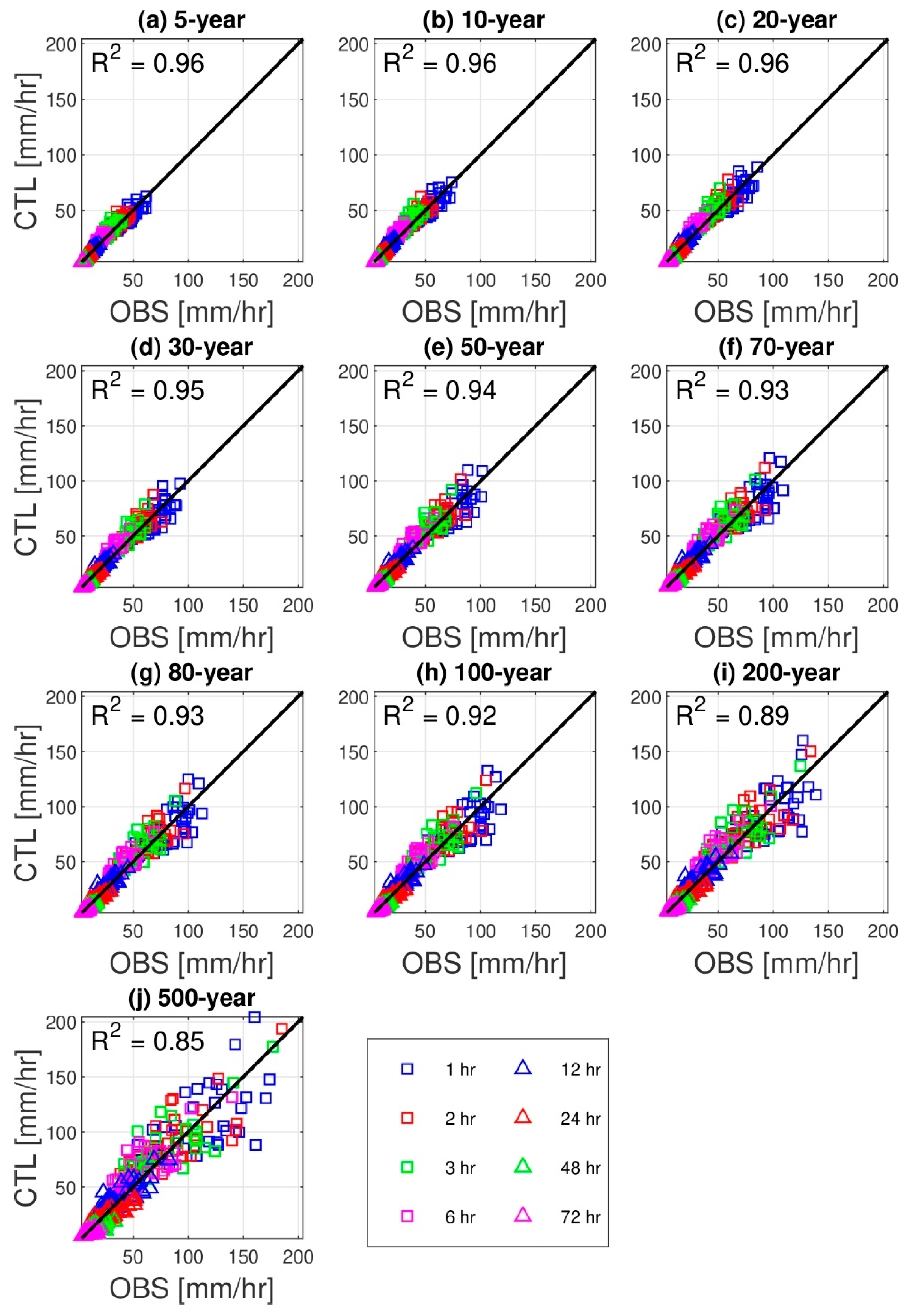
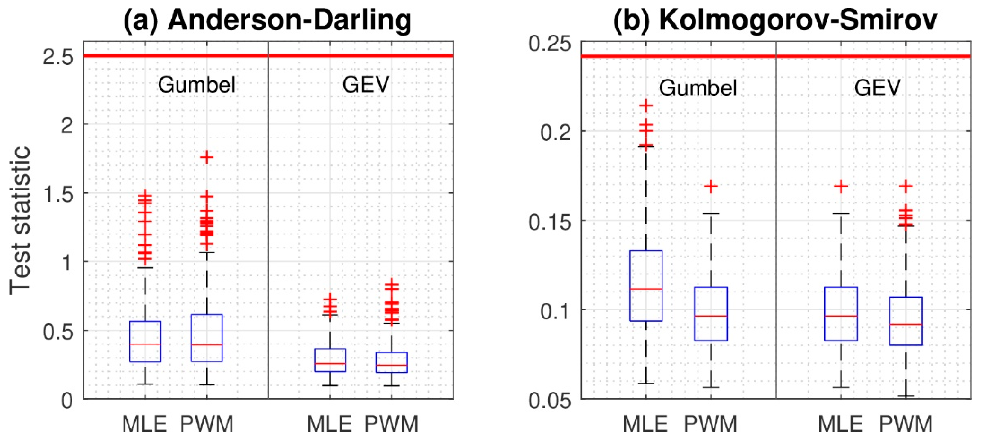
• After obtaining the annual maximum precipitation time series, we selected a probability distribution appropriate for the data and estimated its parameters. Among the common probability distributions applied to frequency analyses of extreme precipitation, such as the lognormal, log-Pearson III, generalized extreme value (GEV), and Gumbel distributions, the GEV distribution is the most popular [6,7,48,49,50]. For South Korea, both the Gumbel [51] and GEV [7] distributions have been recommended. Therefore, we chose the Gumbel and GEV distributions as appropriate to our purposes and then used maximum likelihood estimation and probabilistic weighted moment for parameter estimation. Two goodness-of-fit tests, the Anderson-Darling test [52] and Kolmogorov-Smirnov test [53], were applied to the 2 by 2 combinations to determine whether a given sample came from the hypothesized distribution. Those tests were performed for 1280 cases (2 distributions × 2 parameter estimation methods × 8 durations × 40 locations).
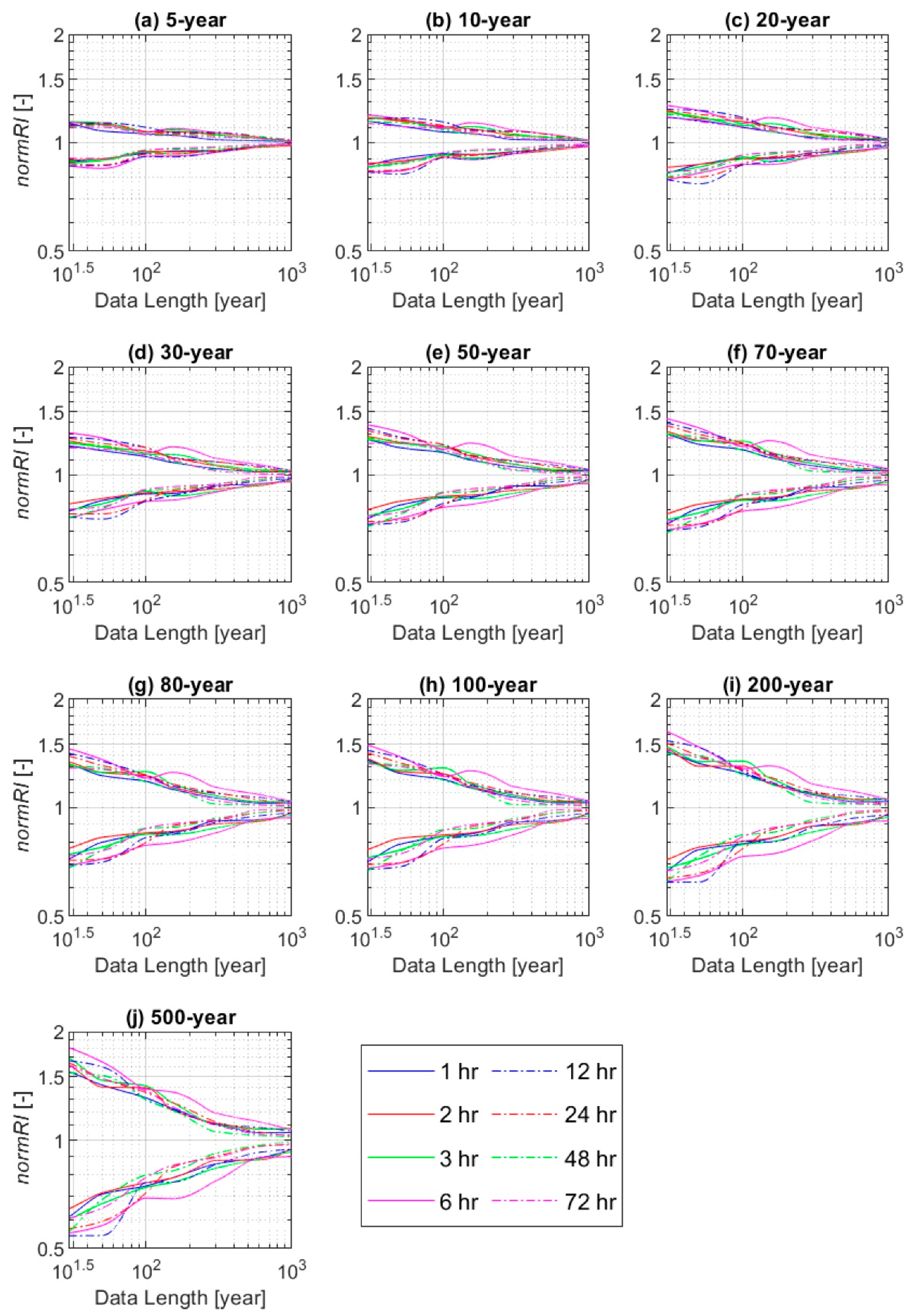
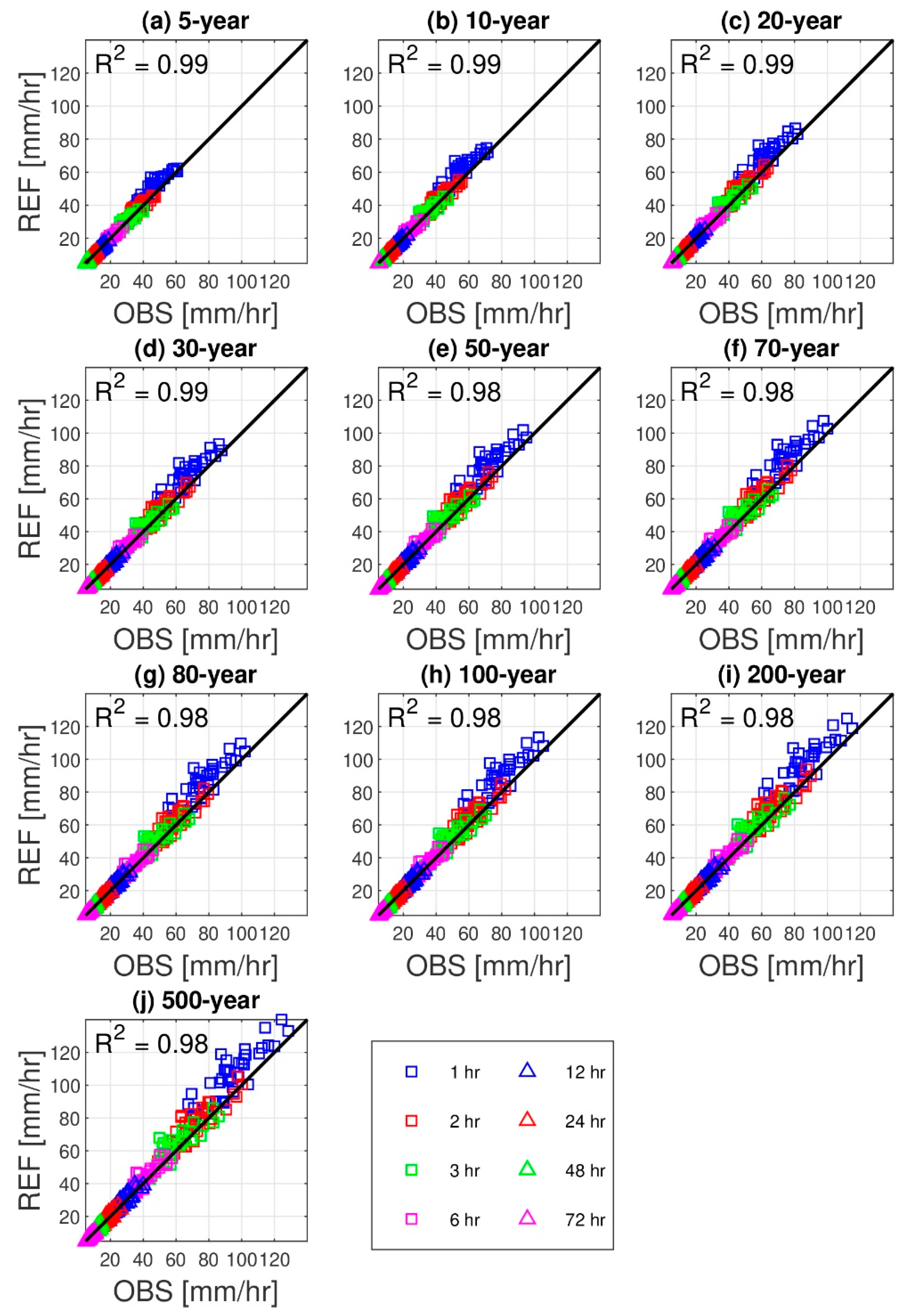
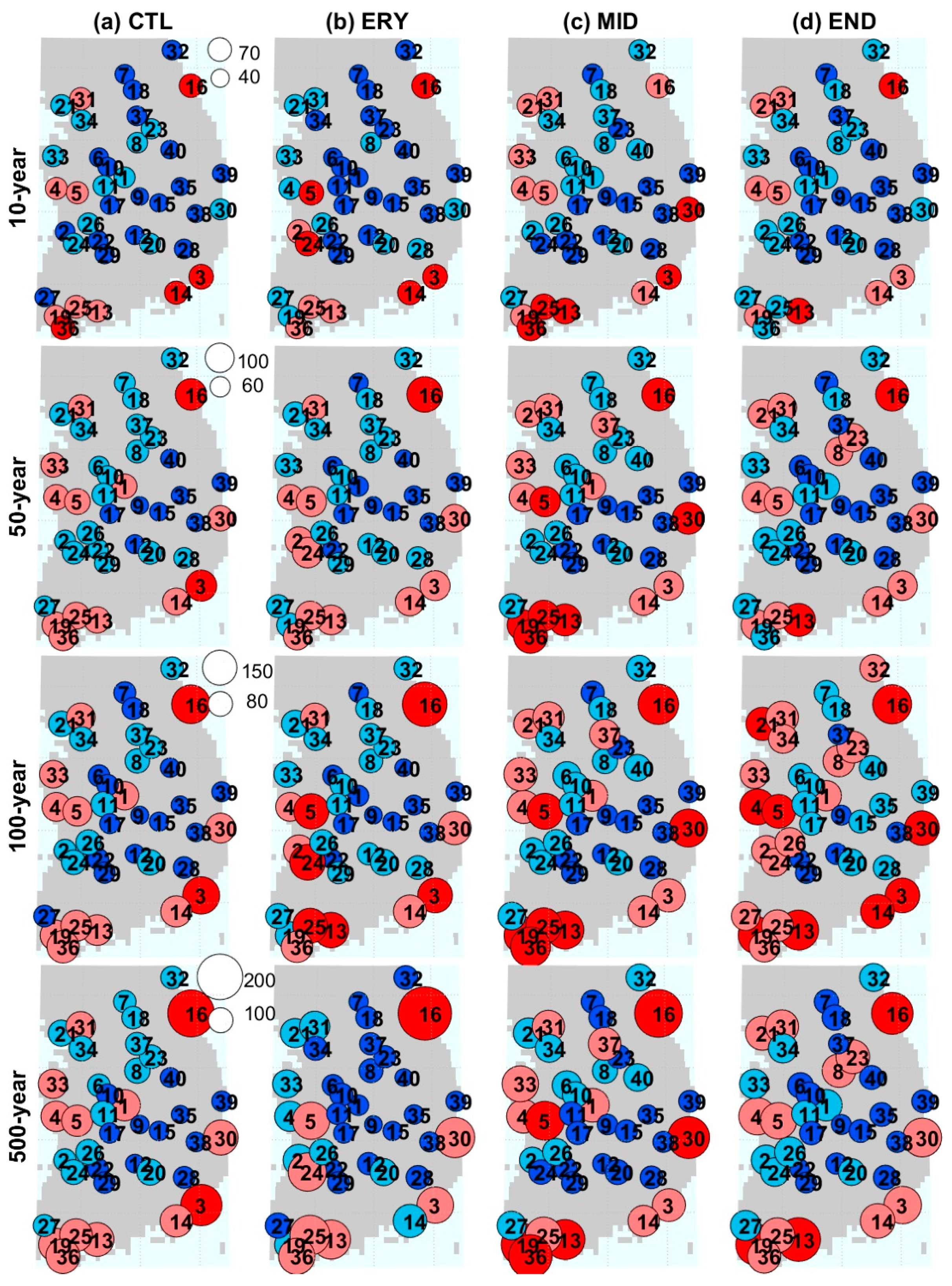
• The precipitation frequency estimates for various durations and return periods were computed from the cumulative distribution function using the estimated parameters of GEV and Gumbel distributions. In this study, 10 return periods (or recurrence intervals) of 5, 10, 20, 30, 50, 70, 80, 100, 200, and 500 years were considered. In total, the precipitation estimates were calculated for 10 return periods × 8 durations × 100 ensemble members × 40 locations.
• We then repeated Steps 3 to 7 for the control (CTL) and 3 future periods (ERY, MID, and END) and 2 RCP scenarios (RCP 4.5 and RCP 8.5) to assess our changing precipitation frequency estimates for the future. The total number of precipitation frequency estimates calculated was 10 return periods × 8 durations × 700 ensemble members × 40 locations.
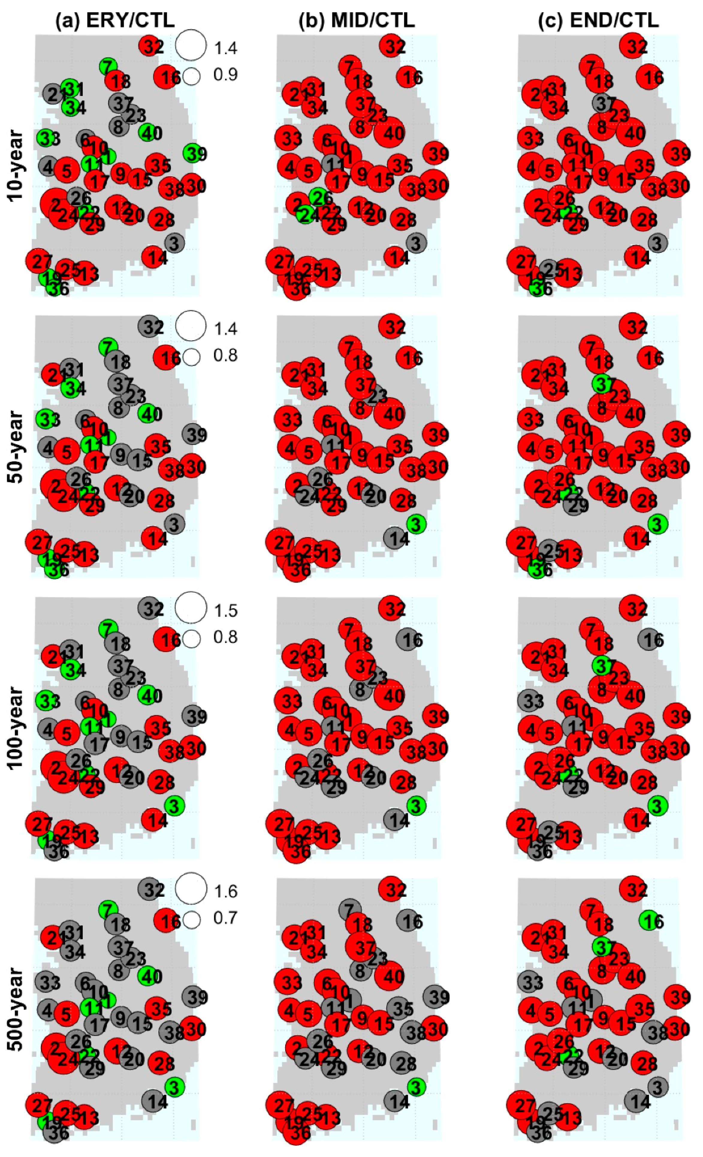
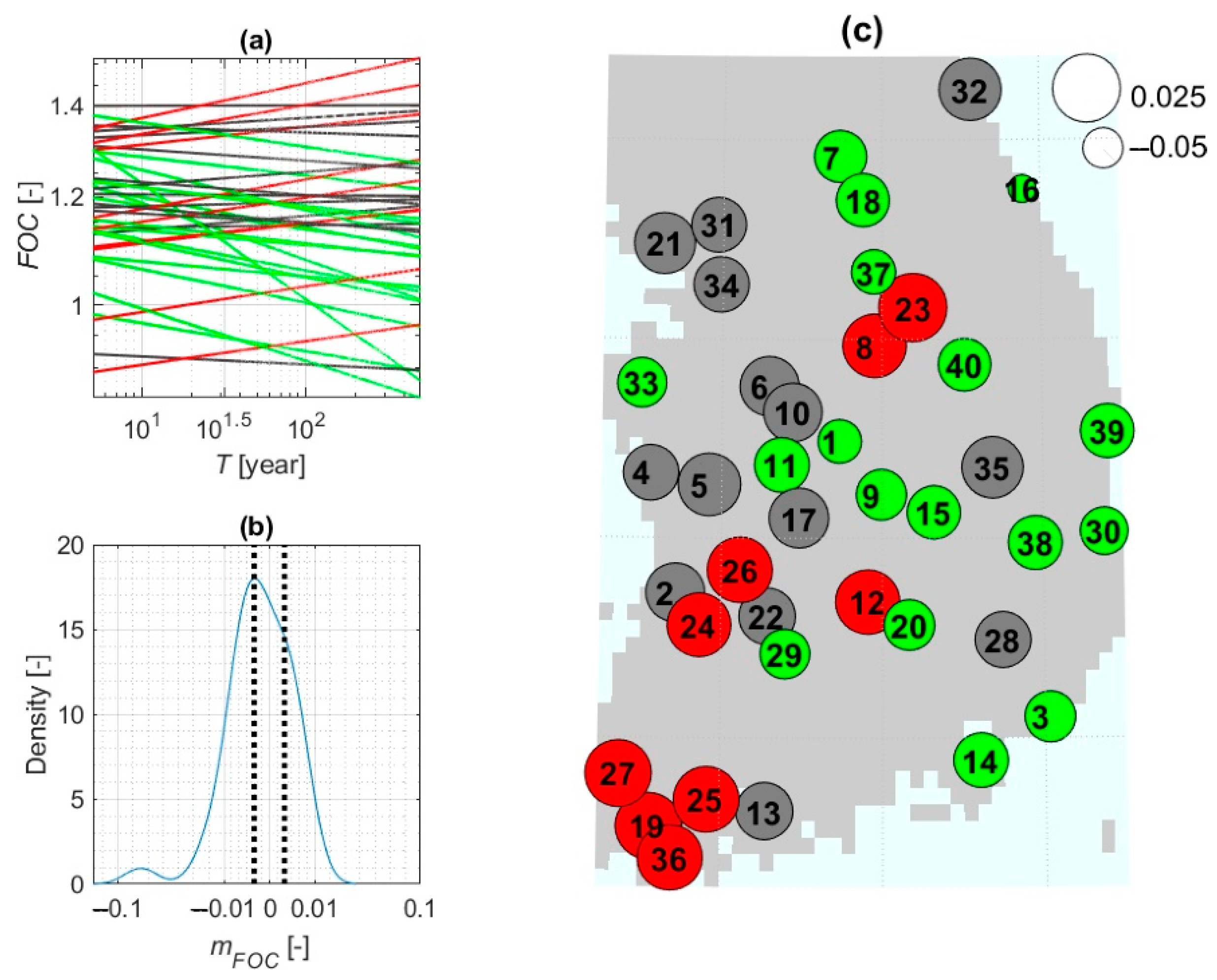
• To assess changes in the rainfall frequency estimates between the control and future periods for a given duration and return period, the FOC was introduced as the ratio of future rainfall intensity to the control intensity using the average value of 100 ensembles. Thus, the FOC represents how much the rainfall frequency estimate for a specific duration and return period increases or decreases in future periods. The total number of FOCs is 6 comparing pairs × 10 return periods × 8 durations × 40 locations.
• We were able to perform tests of significance for the mean differences between pairs of distributions because the rainfall estimates for each specific duration and return period consisted of 100 values that formed a distribution. That is, we were able to examine the distributions corresponding to the control and each future period to see how they differed from each other. A t-test can be used to test the mean difference between two independent samples with a significance level of 0.05 [54]. The null hypothesis was that the mean of the distributions would not change, and the alternative hypothesis was that they would differ significantly.

3. Results

3.1. Precipitation Frequency Estimates and Their Validation

Choosing an appropriate distribution that fits the data is challenging in a frequency analysis. The GEV and Gumbel distributions were selected because they had been suggested by previous studies in South Korea [7,51]. We estimated their parameters using the maximum likelihood estimation and probabilistic weighted moment methods. Figure 1 shows the statistical results of two goodness-of-fit tests (Anderson-Darling and Kolmogorov-Smirnov), which are compared to the critical values of 2.49 (Anderson-Darling test) [55] and 0.24 (Anderson-Darling test) [56] for 30 samples, with a significance level of 0.05. Because all the test statistics are less than the critical values, all combinations of distributions and parameter estimation methods are appropriate. Nonetheless, in this study, we used the GEV distribution and probabilistic weighted moment method because that combination produced the best results.

To examine the reliability of our results, we compared them with data officially published by the Korean government (hereinafter referred to as REF) [57]. Because the REF results were estimated using maximum likelihood estimation with the Gumbel distribution, we recalculated our results using those methods for this comparison, which is shown in Figure 2. The two sets of results differ very little (the coefficients of determination, R², were 0.98 to 0.99). The reason for the slight discrepancy is that the period and length of data used for the estimations are different. That is, this study consistently uses 30-year data from 1981 to 2010 for all locations (OBS), whereas the REF data length varies from 30 to 79 years. Nonetheless, the high R² value confirms that the rainfall frequency estimates obtained in this study are stable and reliable.

The total precipitation per year varies significantly from one year to another. That variability causes extreme values and increases the uncertainty in the frequency analysis. To quantify that uncertainty when investigating differences between estimates from a short period of observed data (OBS) and those from a long generation period (CTL), we created an ensemble time series using the AWE-GEN stochastic weather generator. As shown in Figure 3, the compared results have R² values in the range of 0.85 to 0.96, indicating a trend that R² decreases as the return period increases. The rainfall frequency estimates close to the median (i.e., smaller return periods) have values that converge, regardless of the sample period, and the uncertainty in the estimate increases as it approaches the extreme percentiles (i.e., larger return periods), which we discuss further in the next section.

3.2. Ensemble Precipitation Frequency Estimates for Control and Future Periods

In this study, precipitation frequency estimates (or rainfall intensities) have been computed for a range of return periods and durations for each location in the control and future periods. Overall, the precipitation estimate increases in the future for most locations—their kernel distributions for future periods are shifted on the right, compared with the control period (Figure S1). First, we want to know the spatial distribution and pattern of the calculated precipitation frequency estimates. Figure 4 and Table S2 show the relative sizes of the estimates at all 40 locations, which were classified into distinctive regions by applying the k-means cluster algorithm. The number of clusters, k = 4, was chosen according to the Elbow method [34]. The results in Figure 4 show that the stations with high precipitation frequency estimates (light red and red circles) are mostly in coastal areas, and those with low estimates are in the central inland areas of South Korea. Therefore, the IDF curves of the coastal and central inland regions (e.g., Gangneung (No. 16) and Chupungnyeong (No. 9), respectively; Figure S2) are quite different. Note that these IDF curves are proportional to the return periods and inversely proportional to the durations—which is consistent with typical IDF results. These spatial patterns are consistent for all return periods, durations, and future periods, and they were also observed with the RCP 4.5 scenario (Figure S3).

We further found that the spatial distribution of the precipitation frequency estimates was similar to that of the CM and CIV. In particular, for the indices of maximum daily (maxDa) and hourly (maxHr) precipitation, which are related to extremes (see Figure 3 and Figure 5 in Van Doi and Kim [17]), regions with high CM and CIV values are in the coastal areas of South Korea, and the central inland areas have lower CM and CIV values. Therefore, locations with high CM and CIV values also have high precipitation estimates.

It is important to understand the effects of the anthropogenic factors accelerating climate change (e.g., the amount of greenhouse gas emissions or the extent of future economic growth). In this study, precipitation frequency estimates were calculated for two emissions scenarios (RCP 4.5 and RCP 8.5). How the RCP 8.5 estimates differ from the RCP 4.5 estimates was evaluated by applying the t-test. The results indicate that the effects of RCP tend to be complex; its effects can be great (red circles) or small (green circles), or it can have no effect (grey circles in Figure S4), depending on the future time and location.

3.3. Factors of Change for Precipitation Frequency Estimates

To present a quantitative value for future changes in precipitation frequency estimates, we calculated product type FOCs and spatially represented their relative magnitudes using the size of each circle in Figure 5. The values of factor of change (FOC) for each location can be also found in Table S3. Additionally, we conducted t-testing to confirm that the computed FOCs differ significantly from the present one, and those results are indicated by the color of the circles in Figure 5. Clearly, the future estimates can significantly increase (red circles), decrease (green circles), or remain unchanged (grey circles), but, at most locations (especially for the END period), the future estimates increase significantly from current observations. This phenomenon was also observed for other durations (not shown) and the RCP 4.5 scenario (Figure S5).

Some clustered locations currently have similar precipitation frequency estimates, but their future changes could vary significantly. For example, the CTL estimates in Hongcheon (No. 18) and Wonju (No. 37), which are only ~50 km apart, had similar values of 47.41 mm/h and 47.57 mm/h, respectively, for a 1-h duration and a 10-year return period. However, in the END period, those values decrease slightly in Wonju (FOC = 0.985) and increase significantly in Hongcheon (FOC = 1.216). Thus, it is risky to estimate future changes in precipitation frequency for a location by using a nearby station with a similar present precipitation frequency estimate. In other words, when investigating future changes in precipitation frequency estimates, data should not be regionalized.

4. Discussion

4.1. Do the Tail Characteristics of Future Extreme Rainfall Distribution Change?

One interesting question is whether the tail characteristics of future extreme rainfall distributions will remain the same as those found now. Looking at a typical IDF equation, such as Equation (1), rainfall intensity, RI (precipitation frequency estimate), is proportional to frequency, T (return period), and inversely proportional to duration, D [58]. It is well known that the intensity increases exponentially (the exponent, m is always positive) as the frequency increases, but it is also important to note that the degree to which it increases varies from region to region.

$$RI=\frac{a{T}^m}{{\left(b+D\right)}^n},$$

(1)

where a, b, m, and n are location-dependent coefficients. For a fixed duration, this equation is simply expressed as:

$$RI=c{T}^m,$$

(2)

where c is a coefficient. The coefficient m, the slope of the linear regression relationship on the logarithmic scale, represents the degree to which the precipitation frequency estimates increase over the return period. A steeper slope in Figure 6a infers that the right tail of the extreme rainfall distribution is longer. That slope value varies by region and ranges from 0.123 to 0.224 in South Korea (Figure 6b). An interesting result was observed: the spatial distribution of the slope values is similar to that of the precipitation frequency estimates (Figure 4d and Figure 6c). In other words, if the 10-year frequency estimate in a region is relatively high, the upward pattern of the estimate for increasing frequency is also high. For example, Gangneung (No. 16), which belongs to a relatively high estimate zone, has a high slope (m = 0.194), whereas Chupungnyeong (No. 9), which belongs to a lower estimate zone, has a small slope (m = 0.144). That phenomenon was also observed for other durations and future periods (Figure S6).

A straightforward way to reveal whether the tail characteristics of future extreme rainfall estimates are the same as those for the present estimates is to inspect the slope value of the FOC. Given a fixed duration, the rainfall intensities for the control and future periods are:

$$R{I}_{CTL}=c_{CTL}{T}^{m_{CTL}},$$

(3)

$$R{I}_{FUT}=c_{FUT}{T}^{m_{FUT}},$$

(4)

where $c_{CTL}$ and $c_{FUT}$ are the coefficients, and $m_{CTL}$ and $m_{FUT}$ are the slopes of the control and future periods on the logarithmic scale, respectively. The FOC of the precipitation frequency estimates is computed as:

$$FOC=\frac{R{I}_{FUT}}{R{I}_{CTL}}=c_{FOC}{T}^{m_{FOC}},$$

(5)

where $c_{FOC}$ is a coefficient computed as $c_{FOC}=c_{FUT}/c_{CTL}$, and $m_{FOC}$ represents a slope on the logarithmic scale computed as $m_{FOC}=m_{FUT}-m_{CTL}$. The mathematical form of this equation is the same as Equation (2), but the physical meaning is dissimilar. Unlike in Equation (2), the slope in Equation (5) is not always positive; it can also be negative or close to zero depending on the magnitude of the control and future slope values (Figure 7a,b). If the value of $m_{FOC}$ is far from zero, the tail characteristics for the present and future are quite different. On the other hand, if $m_{FOC}$ is close to zero, the values of $m_{FUT}$ and $m_{CTL}$ are similar. The latter indicates that those tail characteristics are comparable, and the FOC value can remain constant for any duration, regardless of frequency.

In the context of climate change, FOC values are commonly used to express how much the annual maximum precipitation in the future will differ from that in the present. Can those same FOC values be used to compute estimates that correspond to the median and the tails? Put another way, can the FOCs for small return periods be identical to those for larger return periods? The answer can be yes (if $m_{FOC}$ is close to zero) or no (if $m_{FOC}$ is far from zero), depending on the region. In South Korea, some locations, such as Imsil (No. 22), have values of $m_{FOC}$ that are approximately equal to zero (−0.0058), whereas others, such as Namwon (No. 29) and Jeonju (No. 26), have values of −0.0248 and 0.0177 (Figure 7c for 1-h duration and END period, Figure S7 for other cases). Note that those three locations are all close together. Therefore, it is important to mind the tail characteristics when designing water infrastructure to determine whether they change in the future.

4.2. Do Short-Range Data Provide Reliable Precipitation Frequency Estimates?

Predictions inevitably carry uncertainties, but a good understanding and quantification of those uncertainties can reduce risk when making decisions and proposing mitigation measures. One uncertainty that can arise when calculating precipitation frequency estimates is the amount of data used. If the data collection period is long enough, making predictions for longer return periods will be straightforward. However, many areas have limited records, so it is unfeasible to collect sufficient data. Therefore, it is necessary to identify how much uncertainty is included in rainfall intensity estimates derived from a limited range of data.

In this study, we used the AWE-GEN stochastic weather generator to create 100 ensembles of 30-year time series that reflect CIV corresponding to 3000 years to quantify the uncertainty when a shorter period of data was used. Figure 8 shows the magnitude of the uncertainty when using short-term data by using rainfall intensities normalized by their ensemble averages (normRI) to facilitate the comparison of rainfall estimates for 8 durations and 10 return periods. Their uncertainty ranges are displayed from the normRI of ensembles 100, 60, 30, 20, 10, 5, and 3 for data lengths of 30, 50, 100, 150, 300, 600, and 1000 years, respectively. As expected, the range of uncertainty is large when the data length is short and gradually decreases as the data length increases, eventually converging to a single point. This tendency is the same for all return periods, but the uncertainty range becomes much greater when estimating RI for a large return period (Figure 9a); for example, depending on the location, the range with a data length of 30 years is 0.18 to 0.30 for a 5-year return period and 0.70 to 1.60 for a 500-year return period. Thus, the uncertainty range is proportional to the return period, but the degree of its increase over the return period depends on the location (Figure 9b,c). As the frequency (T) increases, some locations have a large increase in the range of uncertainty, whereas others have smaller increases. That phenomenon is also valid for other durations and future periods (Figure S8).

Short-range data cannot provide reliable rainfall estimates, especially for very rare events. If only a short range of data is available, the uncertainty by which the estimates deviate from the converging average can be quantified by generating an ensemble that embraces natural stochasticity.

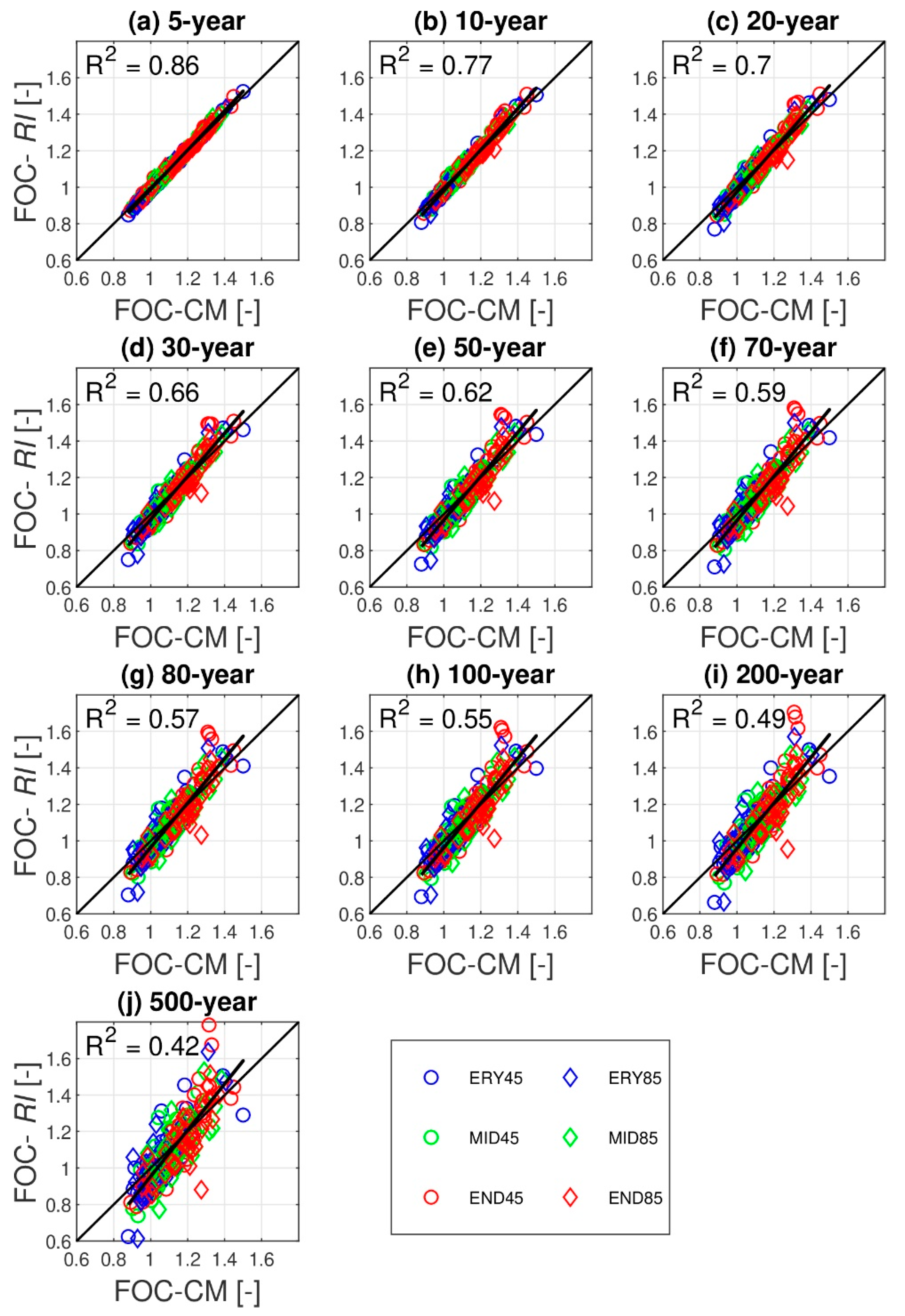
4.3. Is It Feasible to Infer Future Changes in RI from Those of Climatological Mean?

In climate studies, the CM, often calculated as a 30-year average, is a common climate indicator [17,37,38,39,40,41]. Predicting the FOC of the CM is easier than predicting that of extreme percentiles (RI) because even short periods of data can provide a reasonably stable convergence value for the CM. Therefore, it is important to investigate whether it is possible to infer the FOC of RI using only the FOC for the CM and (if so) how much uncertainty the inference will contain.

We already confirmed that the FOC can be frequency-independent in several locations (grey circles in Figure 7). At those locations, the FOCs of the CM and RI are the same ($m_{FOC}$is close to zero); thus, the FOC of RI can be sufficiently inferred from the FOC of the CM. However, in locations with non-zero $m_{FOC}$values, the FOCs of the CM and RI can differ significantly. Figure 10 shows 1:1 relationships for all locations and all future periods. As expected, for smaller return periods, the FOC of RI correlates highly with the FOC of the CM (R² = 0.86 for the 5-year return period); on the other hand, R² falls to 0.42 for rare rainfall events (e.g., a 500-year return period). This reduction in R² values at longer return periods is because the cumulative distribution function for the annual maximum precipitation does not shift in parallel in some scenarios and locations. That is, the rainfall characteristics of the tail part of the cumulative distribution can vary with greater uncertainty than its body part. If the FOC of RI must be estimated using the FOC of the CM, a longer return period correlates with greater uncertainty in the FOC of RI. For example, when the FOC of the CM is 1.2, the FOC of RI is 1.18 to 1.22 for a 5-year return period but 1.0 to 1.5 for a 500-year return period, which is a much greater range of uncertainty.

Similar to Figure 10, which shows the results for a 1-h duration, the same conclusion can be made for events with a 24-h duration (Figure S9). However, in the latter case, the predictive power of inferring the FOC of RI from the FOC of the CM is stronger (R² = 0.56 to 0.98).

5. Conclusions

To address CIV and tail characteristics with respect to the return period when developing future IDF curves, this study used the AWE-GEN stochastic weather generator to produce ensembles of 30-year hourly precipitation time series for control and future periods using two different emission scenarios across 40 locations in South Korea. To calculate the ensembles, the GEV distribution and probabilistic weighted moment method were chosen based on the statistical results from the goodness-of-fit tests. Precipitation frequency estimates were calculated for 10 return periods × 8 durations × 700 ensemble members × 40 locations. We examined our estimates by comparing them with those officially published by the Korean government. R² values ranging from 0.98 to 0.99 confirm that our rainfall frequency estimates are stable and reliable.

We computed precipitation frequency estimates for each location for a range of durations and return periods in the control and future periods and found that (1) the future precipitation frequency estimates increase significantly for most locations (especially during the END period); (2) the spatial distributions and patterns of the precipitation frequency estimates indicate that stations in coastal areas have high estimates, whereas those in the central inland areas of South Korea have low estimates; (3) the spatial distributions and patterns of the precipitation frequency estimates are also similar to those of the CM and CIV, allowing the pattern of precipitation estimates to be inferred from the mean and variability patterns of rainfall distribution; and (4) different emission scenarios will have large, small, or no effects, depending on location and time into the future.

It is interesting to investigate whether the tail characteristics of future extreme rainfall events will remain the same as those in the present. Using a typical IDF equation, we focused on the coefficient m, the slope of the linear regression relationship on the logarithmic scale, which represents the degree to which the precipitation frequency estimates increase across return periods given a fixed duration. That is, having a steep slope in Figure 6a implies that the right tail of the extreme rainfall distribution is long. That slope value varies by region and ranges from 0.123–0.224 in South Korea. A more straightforward way to reveal whether the tail characteristics for future extreme rainfall events are the same as they are at present is to inspect the slope value for the FOC. Conclusively, the tail characteristics in the present and future differ when the $m_{FOC}$ value is far from zero, and they are similar when the $m_{FOC}$ value is close to zero. Therefore, the $m_{FOC}$ value is an important key to determining whether the same FOC values can be used for small and large return periods.

An important thing to note is that future changes in precipitation frequency estimates should not be regionalized to values of nearby stations. In this regard, we report two interesting findings. Some nearby locations currently have similar precipitation frequency estimates but quite different future changes (FOCs). Furthermore, some locations are clustered together, but their tail characteristics with respect to the return period ($m_{FOC}$) are dissimilar. Therefore, regionalizing with nearby values is very risky when investigating future changes in precipitation frequency estimates.

A limited range of data is one source of uncertainty when computing precipitation frequency estimates. That type of uncertainty needs to be quantified when only short-range data are available. A short range of data (e.g., 30 years) offers just one of many realizations that occurred in the past or will occur in the future; thus, it cannot sufficiently explain CIV. Using an ensemble that corresponds to very long data lengths is a good way to predict the uncertainty inherent in CIV. In this study, 100 ensembles were created for a 30-year time series to quantify that uncertainty. As expected, the magnitude of uncertainty was large when the data length was short, and it gradually decreased as the data length increased. That tendency was the same for all return periods, but the uncertainty range became much greater for large return periods, for example, depending on the location, the range with a data length of 30 years was 0.18 to 0.30 for a 5-year return period and 0.70 to 1.60 for a 500-year return period (Figure 9a).

Predicting the FOC of the CM is easier than predicting that of extreme percentiles (RI) because even short periods of data provide a reasonably stable convergence value for the CM. Thus, the question becomes whether it is possible to infer the FOC of RI using only the FOC of the CM and (if so) how much uncertainty the inference will contain. We found that inferring future changes in RI from those in the CM is feasible for small return periods and at locations where $m_{FOC}$is close to zero. However, it is a risky strategy for large return periods or at locations with non-zero $m_{FOC}$values because the uncertainty is greater in those circumstances.

It is important to quantify and assess future changes in precipitation frequency estimates and their uncertainty. The findings of this study will complement the assessment of future changes in precipitation frequency estimates in the context of climate change, and they provide useful information at a fine temporal scale for designing water infrastructure.

References

1. Milly, P.C.D.; Betancourt, J.; Falkenmark, M.; Hirsch, R.M.; Kundzewicz, Z.W.; Lettenmaier, D.P.; Stouffer, R.J. Climate change. Stationarity is dead: Whither water management? Science 2008, 319, 573–574. [Google Scholar] [CrossRef]
2. Cheng, L.; AghaKouchak, A.; Gilleland, E.; Katz, R. Non-stationary extreme value analysis in a changing climate. Clim. Chang. 2014, 127, 353–369. [Google Scholar] [CrossRef]
3. Yilmaz, A.G.; Perera, B.J.C. Extreme Rainfall Nonstationarity Investigation and Intensity–Frequency–Duration Relationship. J. Hydrol. Eng. 2014, 19, 1160–1172. [Google Scholar] [CrossRef] [Green Version]
4. DeGaetano, A.T.; Castellano, C.M. Future projections of extreme precipitation intensity-duration-frequency curves for climate adaptation planning in New York State. Clim. Serv. 2017, 5, 23–35. [Google Scholar] [CrossRef]
5. Cheng, L.; AghaKouchak, A. Nonstationary Precipitation Intensity-Duration-Frequency Curves for Infrastructure Design in a Changing Climate. Sci. Rep. 2014, 4, 7093. [Google Scholar] [CrossRef] [PubMed] [Green Version]
6. Sarhadi, A.; Soulis, E.D. Time-varying extreme rainfall intensity-duration-frequency curves in a changing climate. Geophys. Res. Lett. 2017, 44, 2454–2463. [Google Scholar] [CrossRef]
7. Lima, C.H.; Kwon, H.-H.; Kim, Y.-T. A local-regional scaling-invariant Bayesian GEV model for estimating rainfall IDF curves in a future climate. J. Hydrol. 2018, 566, 73–88. [Google Scholar] [CrossRef]
8. Güçlü, Y.S. Multiple Şen-innovative trend analyses and partial Mann-Kendall test. J. Hydrol. 2018, 566, 685–704. [Google Scholar] [CrossRef]
9. Vu, M.T.; Raghavan, V.S.; Liong, S.-Y. Deriving short-duration rainfall IDF curves from a regional climate model. Nat. Hazards 2016, 85, 1877–1891. [Google Scholar] [CrossRef]
10. Müller, H.; Haberlandt, U. Temporal rainfall disaggregation using a multiplicative cascade model for spatial application in urban hydrology. J. Hydrol. 2018, 556, 847–864. [Google Scholar] [CrossRef]
11. Fadhel, S.; Rico-Ramirez, M.A.; Han, D. Uncertainty of Intensity–Duration–Frequency (IDF) curves due to varied climate baseline periods. J. Hydrol. 2017, 547, 600–612. [Google Scholar] [CrossRef] [Green Version]
12. Li, J.; Johnson, F.; Evans, J.; Sharma, A. A comparison of methods to estimate future sub-daily design rainfall. Adv. Water Resour. 2017, 110, 215–227. [Google Scholar] [CrossRef]
13. Shahabul Alam, M.; Elshorbagy, A. Quantification of the climate change-induced variations in Intensity–Duration–Frequency curves in the Canadian Prairies. J. Hydrol. 2015, 527, 990–1005. [Google Scholar] [CrossRef]
14. Westra, S.; Evans, J.; Mehrotra, R.; Sharma, A. A conditional disaggregation algorithm for generating fine time-scale rainfall data in a warmer climate. J. Hydrol. 2013, 479, 86–99. [Google Scholar] [CrossRef] [Green Version]
15. Pendergrass, A.G.; Knutti, R.; Lehner, F.; Deser, C.; Sanderson, B. Precipitation variability increases in a warmer climate. Sci. Rep. 2017, 7, 1–9. [Google Scholar] [CrossRef] [Green Version]
16. Prein, A.F.; Rasmussen, R.M.; Ikeda, K.; Liu, C.; Clark, M.P.; Holland, G.J. The future intensification of hourly precipitation extremes. Nat. Clim. Chang. 2016, 7, 48–52. [Google Scholar] [CrossRef]
17. Van Doi, M.; Kim, J. Projections on climate internal variability and climatological mean at fine scales over South Korea. Stoch. Environ. Res. Risk Assess. 2020, 34, 1037–1058. [Google Scholar] [CrossRef]
18. Westra, S.J.; Fowler, H.; Evans, J.; Alexander, L.; Berg, P.; Johnson, F.; Kendon, E.J.; Lenderink, G.; Roberts, N.M. Future changes to the intensity and frequency of short-duration extreme rainfall. Rev. Geophys. 2014, 52, 522–555. [Google Scholar] [CrossRef]
19. Tran, V.N.; Dwelle, M.C.; Sargsyan, K.; Ivanov, V.Y.; Kim, J. A Novel Modeling Framework for Computationally Efficient and Accurate Real-Time Ensemble Flood Forecasting With Uncertainty Quantification. Water Resour. Res. 2020, 56, 1–31. [Google Scholar] [CrossRef]
20. Kim, J.; Ivanov, V.Y.; Fatichi, S. Environmental stochasticity controls soil erosion variability. Sci. Rep. 2016, 6, 22065. [Google Scholar] [CrossRef] [Green Version]
21. Kim, J.; Ivanov, V.Y.; Fatichi, S. Soil erosion assessment-Mind the gap. Geophys. Res. Lett. 2016, 43, 12446–12456. [Google Scholar] [CrossRef]
22. Cannon, A.J.; Innocenti, S. Projected intensification of sub-daily and daily rainfall extremes in convection-permitting climate model simulations over North America: Implications for future intensity–duration–frequency curves. Nat. Hazards Earth Syst. Sci. 2019, 19, 421–440. [Google Scholar] [CrossRef] [Green Version]
23. Moustakis, Y.; Papalexiou, S.M.; Onof, C.J.; Paschalis, A. Seasonality, Intensity, and Duration of Rainfall Extremes Change in a Warmer Climate. Earth’s Futur. 2021, 9, 1–15. [Google Scholar] [CrossRef]
24. Nerantzaki, S.D.; Papalexiou, S.M. Tails of extremes: Advancing a graphical method and harnessing big data to assess precipitation extremes. Adv. Water Resour. 2019, 134, 103448. [Google Scholar] [CrossRef]
25. Papalexiou, S.M.; AghaKouchak, A.; Foufoula-Georgiou, E. A Diagnostic Framework for Understanding Climatology of Tails of Hourly Precipitation Extremes in the United States. Water Resour. Res. 2018, 54, 6725–6738. [Google Scholar] [CrossRef]
26. Hawkins, E.; Sutton, R. The potential to narrow uncertainty in projections of regional precipitation change. Clim. Dyn. 2010, 37, 407–418. [Google Scholar] [CrossRef]
27. Deser, C.; Phillips, A.; Bourdette, V.; Teng, H. Uncertainty in climate change projections: The role of internal variability. Clim. Dyn. 2010, 38, 527–546. [Google Scholar] [CrossRef] [Green Version]
28. Deser, C.; Phillips, A.S.; Alexander, M.; Smoliak, B. Projecting North American Climate over the Next 50 Years: Uncertainty due to Internal Variability. J. Clim. 2014, 27, 2271–2296. [Google Scholar] [CrossRef] [Green Version]
29. Fischer, E.M.; Sedlacek, J.; Hawkins, E.; Knutti, R. Models agree on forced response pattern of precipiation and temperature extremes. Geophys. Res. Lett. 2014, 41, 8554–8562. [Google Scholar] [CrossRef] [Green Version]
30. Hingray, B.; Saïd, M. Partitioning Internal Variability and Model Uncertainty Components in a Multimember Multimodel Ensemble of Climate Projections. J. Clim. 2014, 27, 6779–6798. [Google Scholar] [CrossRef]
31. Martel, J.-L.; Mailhot, A.; Brissette, F.; Caya, D. Role of Natural Climate Variability in the Detection of Anthropogenic Climate Change Signal for Mean and Extreme Precipitation at Local and Regional Scales. J. Clim. 2018, 31, 4241–4263. [Google Scholar] [CrossRef]
32. Kim, J.; Ivanov, V.Y. A holistic, multi-scale dynamic downscaling framework for climate impact assessments and challenges of addressing finer-scale watershed dynamics. J. Hydrol. 2015, 522, 645–660. [Google Scholar] [CrossRef] [Green Version]
33. Kim, J.; Ivanov, V.Y.; Fatichi, S. Climate change and uncertainty assessment over a hydroclimatic transect of Michigan. Stoch. Environ. Res. Risk Assess. 2015, 30, 923–944. [Google Scholar] [CrossRef]
34. Kim, J.; Tanveer, M.E.; Bae, D.-H. Quantifying climate internal variability using an hourly ensemble generator over South Korea. Stoch. Environ. Res. Risk Assess. 2018, 32, 3037–3051. [Google Scholar] [CrossRef]
35. Deser, C.; Hurrell, J.W.; Phillips, A.S. The role of the North Atlantic Oscillation in European climate projections. Clim. Dyn. 2016, 49, 3141–3157. [Google Scholar] [CrossRef]
36. Wang, J.; Bessac, J.; Kotamarthi, R.; Constantinescu, E.; Drewniak, B. Internal variability of a dynamically downscaled climate over North America. Clim. Dyn. 2017, 50, 4539–4559. [Google Scholar] [CrossRef]
37. Kang, I.-S.; Shukla, J. Dynamic seasonal prediction and predictability of the monsoon. In The Asian Monsoon; Wang, B., Ed.; Springer: Berlin/Heidelberg, Germany, 2006; pp. 585–612. [Google Scholar] [CrossRef]
38. Peleg, N.; Molnar, P.; Burlando, P.; Fatichi, S. Exploring stochastic climate uncertainty in space and time using a gridded hourly weather generator. J. Hydrol. 2019, 571, 627–641. [Google Scholar] [CrossRef]
39. Fatichi, S.; Ivanov, V.Y.; Paschalis, A.; Peleg, N.; Molnar, P.; Rimkus, S.; Kim, J.; Burlando, P.; Caporali, E. Uncertainty partition challenges the predictability of vital details of climate change. Earth’s Futur. 2016, 4, 240–251. [Google Scholar] [CrossRef]
40. Fischer, E.; Beyerle, U.; Knutti, R. Robust spatially aggregated projections of climate extremes. Nat. Clim. Chang. 2013, 3, 1033–1038. [Google Scholar] [CrossRef]
41. Giorgi, F.; Mearns, L.O. Calculation of average, uncertainty range, and reliability of regional climate changes from AOGCM simulations via the “reliability ensemble averaging” (REA) method. J. Clim. 2002, 15, 1141–1158. [Google Scholar] [CrossRef]
42. Ivanov, V.Y.; Bras, R.L.; Curtis, D.C. A weather generator for hydrological, ecological, and agricultural applications. Water Resour. Res. 2007, 43, 1–21. [Google Scholar] [CrossRef] [Green Version]
43. Fatichi, S.; Ivanov, V.Y.; Caporali, E. Simulation of future climate scenarios with a weather generator. Adv. Water Resour. 2011, 34, 448–467. [Google Scholar] [CrossRef]
44. Tebaldi, C.; Smith, R.L.; Nychka, D.; Mearns, L.O. Quantifying Uncertainty in Projections of Regional Climate Change: A Bayesian Approach to the Analysis of Multimodel Ensembles. J. Clim. 2005, 18, 1524–1540. [Google Scholar] [CrossRef] [Green Version]
45. Tran, V.; Kim, J. Quantification of predictive uncertainty with a metamodel: Toward more efficient hydrologic simulations. Stoch. Environ. Res. Risk Assess. 2019, 33, 1453–1476. [Google Scholar] [CrossRef]
46. Zhu, J.; Stone, M.C.; Forsee, W. Analysis of potential impacts of climate change on intensity–duration–frequency (IDF) relationships for six regions in the United States. J. Water Clim. Chang. 2012, 3, 185–196. [Google Scholar] [CrossRef]
47. Kim, J.; Lee, J.; Kim, D.; Kang, B. The role of rainfall spatial variability in estimating areal reduction factors. J. Hydrol. 2018, 568, 416–426. [Google Scholar] [CrossRef]
48. Ombadi, M.; Nguyen, P.; Sorooshian, S.; Hsu, K. Developing Intensity-Duration-Frequency (IDF) Curves From Satellite-Based Precipitation: Methodology and Evaluation. Water Resour. Res. 2018, 54, 7752–7766. [Google Scholar] [CrossRef]
49. Ragno, E.; AghaKouchak, A.; Love, C.A.; Cheng, L.; Vahedifard, F.; Lima, C.H.R. Quantifying Changes in Future Intensity-Duration-Frequency Curves Using Multimodel Ensemble Simulations. Water Resour. Res. 2018, 54, 1751–1764. [Google Scholar] [CrossRef]
50. Bairwa, A.K.; Khosa, R.; Maheswaran, R. Developing intensity duration frequency curves based on scaling theory using linear probability weighted moments: A case study from India. J. Hydrol. 2016, 542, 850–859. [Google Scholar] [CrossRef]
51. So, B.-J.; Kim, J.-Y.; Kwon, H.-H.; Lima, C.H. Stochastic extreme downscaling model for an assessment of changes in rainfall intensity-duration-frequency curves over South Korea using multiple regional climate models. J. Hydrol. 2017, 553, 321–337. [Google Scholar] [CrossRef]
52. Anderson, T.W. Anderson–Darling Tests of Goodness-of-Fit. In International Encyclopedia of Statistical Science; Lovric, M., Ed.; Springer: Berlin/Heidelberg, Germany, 2011; pp. 52–54. [Google Scholar]
53. Massey, F.J. The Kolmogorov-Smirnov Test for Goodness of Fit. J. Am. Stat. Assoc. 1951, 46, 68. [Google Scholar] [CrossRef]
54. Lund, R.B.; Von Storch, H.; Zwiers, F.W. Statistical Analysis in Climate Research. J. Am. Stat. Assoc. 2000, 95, 1375. [Google Scholar] [CrossRef] [Green Version]
55. Stephens, M.A. Goodness of Fit for the Extreme Value Distribution. Biometrika 1997, 64, 583–588. [Google Scholar] [CrossRef]
56. Mielke, P.W.; Benjamin, J.R.; Cornell, C.A. Probability, Statistics and Decision for Civil Engineers. J. Am. Stat. Assoc. 1971, 66, 923. [Google Scholar] [CrossRef]
57. MLIT. A Study on the Improvement and Supplement of the Rainfall Probability; Ministry of Land, Infrastructure and Transport: Seoul, Korea, 2011.
58. Chow, V.T.; Maidment, D.R.; Mays, L.W. Applied Hydrology; McGraw-Hill Series in Water Resources and Environmental Engineering; McGraw-Hill: New York, NY, USA, 1988. [Google Scholar]
Figure 1. Goodness of fit tests, (a) Anderson-Darling test and (b) Kolmogorov-Smirnov test for Gumbel and Generalized Extreme Value (GEV) distributions with parameter estimations by the Maximum Likelihood Estimation (MLE) and Probability Weighted Moment (PWM) methods. The number of the boxplot samples for each test is 320 (40 locations × 8 durations). The red line represents the critical value of Anderson-Darling and Anderson-Darling tests (2.49 and 0.24, respectively). On each boxplot, the central mark indicates the median, and the bottom and the top edges of the box indicate the 25th and 75th percentiles, respectively. The ‘+’ symbol represents the outliers, and the whiskers extend to the most extreme data points, not considers outliers.
Water 13 02828 g001
Figure 2. Comparisons of rainfall frequency estimates computed from observation (OBS), from 1981 to 2010 with the reference estimates published by Korean government in the Korea Precipitation Frequency Data Server (REF) for 8 durations and 10 return periods. The number of data points in each subplot is 320 (40 locations × 8 durations). Gumbel distribution and maximum likelihood estimation method are used for both results.
Water 13 02828 g002
Figure 3. Comparisons of rainfall frequency estimates computed from observation (OBS) from 1981 to 2010 with the values averaged for 100 rainfall frequency estimates (CTL) for 8 durations and 10 return periods. The latter estimates are, respectively, computed from 100 AWE-GEN realizations for the same period. The number of data points in each subplot is 320 (40 locations × 8 durations). Generalized Extreme Value distribution and probability weighted moment method are used for both results.
Water 13 02828 g003
Figure 4. Spatial distribution of rainfall frequency estimates over South Korea for the control (CTL) and 3 future periods (ERY, MID, END) with the RCP 8.5 for the 10-, 50-, 100-, and 500-year return periods and 1-h duration. Four clusters from blue (as the smallest cluster), light blue, light red to red (as the largest) are identified after applying the k-means algorithm. The number near white circles is the legend to show the relative magnitude of rainfall estimates.
Water 13 02828 g004
Figure 5. Spatial map of FOC of rainfall frequency estimates at 1-h duration over South Korea for RCP 8.5. The circle size of each location represents the magnitude of FOC. The number near the white circles are used as legends to indicate the relative magnitudes of circles size. A test of significance, t-test is applied to 2 distributions of rainfall frequency estimates in the future and control periods for each location. The dark grey color means that there is no difference between 2 distributions, while red color refers that those increase, and green color refers that those decrease in the future.
Water 13 02828 g005
Figure 6. Varying degree of increase of rainfall frequency estimates (RI) over return periods (T) for 1-h duration for future END period of RCP 8.5. Subplot (a) illustrates the rainfall frequency estimates over return periods for 40 locations. Subplot (b) is a kernel distribution of the slopes (m) for 40 lines in subplot (a). The red (green) lines in subplot (a) refer to locations with their slopes greater (smaller) than mean value—the dark dash lines in subplot (b). Subplot (c) illustrates the spatial distribution of the slope, the colored circles correspond to the colored lines in subplot (a). The number near white circles is the legend to show the relative magnitude of slopes.
Water 13 02828 g006
Figure 7. Future change (FOC) of rainfall frequency estimates over return periods (T) for 1-h duration for future END period of RCP 8.5. Subplot (a) illustrates the FOC of rainfall frequency estimates over return periods for 40 locations. The grey lines have relatively smaller slope values that fall within half the standard deviation with respect to zero—the dark dash lines in subplot (b). The red (green) lines have greater (smaller) slopes than the half standard deviation. Subplot (b) represents a kernel distribution of the slopes of FOC ( m F O C ) for 40 locations in subplot (a). Subplot (c) illustrates the spatial distribution of the slope, the colored circles correspond to the colored lines in subplot (a). The number near white circles is the legend to show the relative magnitude of slopes.
Water 13 02828 g007
Figure 8. Rainfall frequency estimates normalized by their ensemble mean (normRI) for different record lengths of data over 8 durations and 10 return periods in CTL period at the location of Seoul. The below and above lines represent 5th and 95th percentiles of the normRI ensemble, respectively.
Water 13 02828 g008
Figure 9. Varying degree of increase of the uncertainty range (Range), i.e., the difference between 5th and 95th percentiles of the normRI ensemble over return periods (T) for 1-h duration for future END period of RCP 8.5. Subplot (a) illustrates the uncertainty range over return periods for 40 locations. Subplot (b) represents a kernel distribution of the slopes of Range ( m Range ) for 40 lines in subplot (a). The red (green) lines in subplot (a) refer to locations with their slopes greater (smaller) than mean value—the black dashed line in subplot (b). Subplot (c) illustrates the spatial distribution of the slope, the colored circles correspond to the colored lines in subplot (a). The number near white circles is the legend to show the relative magnitude of slopes.
Water 13 02828 g009
Figure 10. Comparisons between the factor of change of climatological mean (FOC-CM) of hourly maximum precipitation with the factor of change of rainfall frequency estimates (FOC-RI) for 1-h duration for 10 return periods. The number of data points is 240 for the subplot (40 locations × 6 comparing periods). The R2 values are computed for the 1:1 line. ERY45, MID45, and END45 are future periods (ERY, MID, and END) with RCP 4.5, respectively. The similarity is for RCP 8.5.
Water 13 02828 g010
Publisher’s Note: MDPI stays neutral with regard to jurisdictional claims in published maps and institutional affiliations.