
Research on Water Quality Simulation and Water Environmental Capacity in Lushui River Based on WASP Model


Abstract
:1. Introduction
2. Materials and Methods
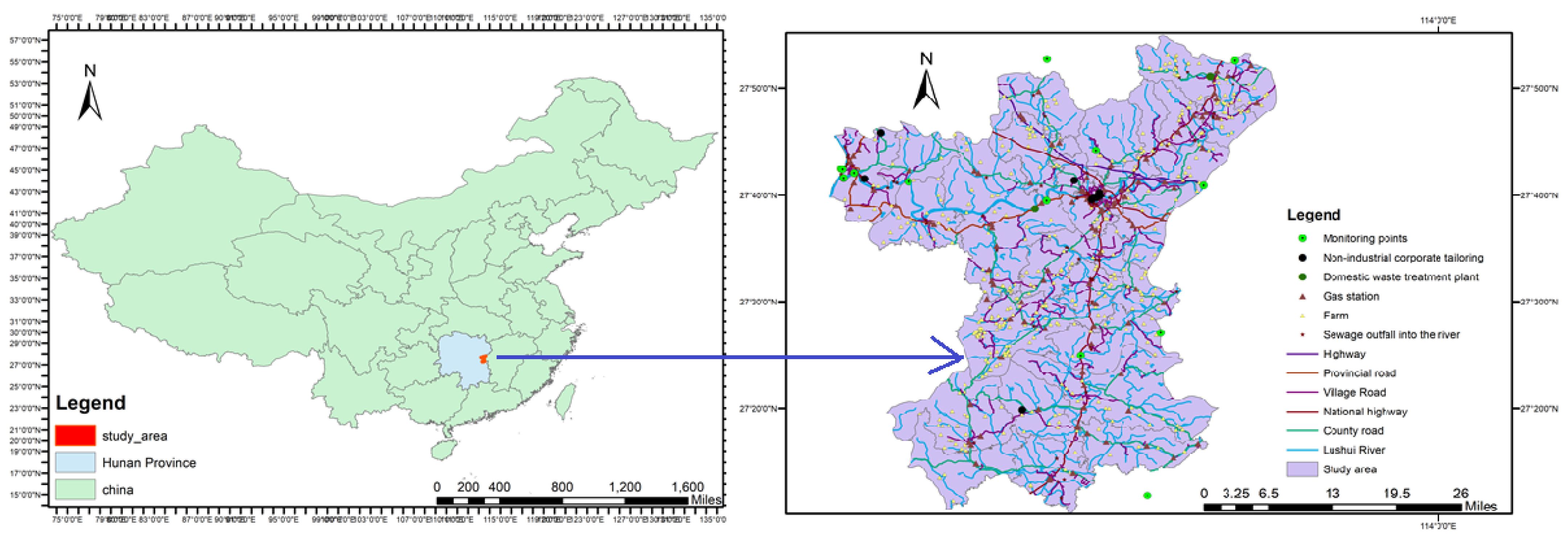
2.1. Case Study
2.2. Determination of the COD, AN and TP
2.3. Model Description and Application
2.4. Model Input
2.4.1. Basic Information
2.4.2. Segmentation and Division of Control Units in the Study Area
- Collection of primary information data of natural geographical features in the Lushui area, including digital elevation (DEM), topographic maps, tributaries, small watershed boundaries, county and city administrative boundaries, environmental function areas, urban built-up areas, companies, drinking water sources, etc.;
- Processing of geographic information data based on ArcGIS, and the above primary geographic information data were overlaid and analyzed. Afterward, a preliminary sketch of the control unit was obtained;
- Division of the control units: after understanding and processing the collected information, the preliminary control unit sketch was fine-tuned according to the control unit’s principles of watershed division and clean boundary. Extraction and confirmation were performed upon the boundaries of different water catchment units and control units on different environmental functions in the same administrative region, to achieve a one-to-one correspondence between pollution source water quality and strong operability;
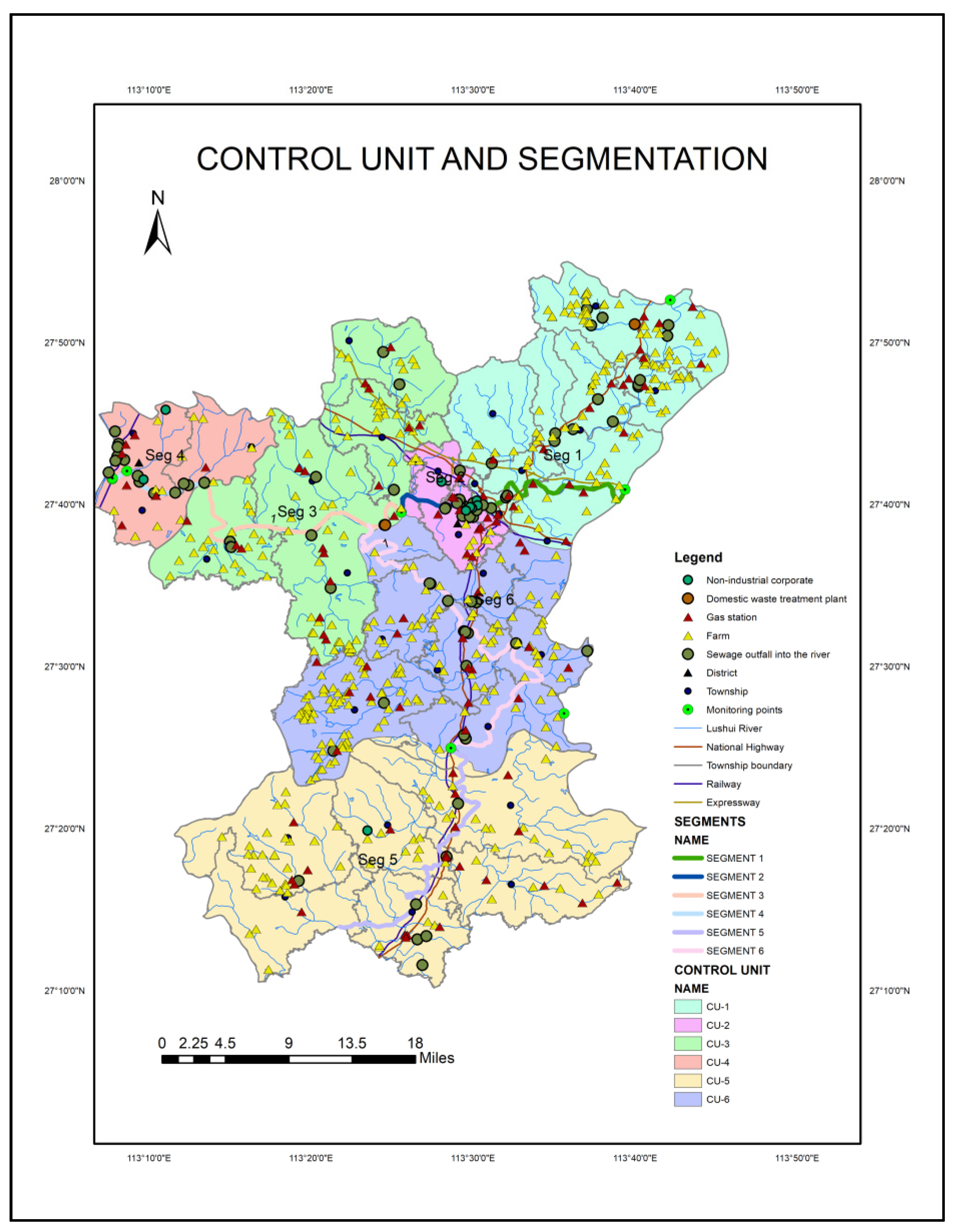
- Naming of the control units: in the absence of nationally unified naming standards and norms, naming was undertaken as a process of trying to understand and conform to the actual situation of each control unit. Therefore, the Lushui River was discretized into six control unit bodies. Each control unit body was given detailed geometric attributes. Some data were obtained from monitoring points during segmentation and generalization. In addition, other geometry parameters were obtained by the formula on WASP 8 User’s Guide. The measured river geometries and water velocities data were used to obtain the value of the exponent and coefficient of velocities and the depth of each segment, as shown in Equations (2), (3), (4), (5) and (6) [12]:B = Bmult × QbexpQm = Vm Dm BmVmult × dmult × bmult = 1where Vm is velocity [m/sec]; Bm is width in m; bmult, Vmult and dmult are empirical coefficients; bexp, vexp and dexp are empirical exponents; and Qm is flow. The flow functions in WASP require the relationships of some hydraulic parameters such as depth and velocity; and the coefficients of the width are obtained internally from Equations 5 and 6. However, in the flow function, the condition of the hydraulic depth exponent, along with width Bm and depth Dm under average flow function, are required. We used Manning’s equation to calculate velocity vm, and the average flow Qm, from width and depth. The segmentation and the division of the control unit in Lushui River are shown in Figure 2 and Table 1.vexp + dexp + bexp = 1
2.4.3. Pollution Load
2.4.4. Discrete Exchange
2.4.5. Initial and Boundary Conditions
2.5. Sensitivity Analysis and Calibration of Parameters
2.5.1. Sensitivity Analysis of Parameters
- Local sensitivity analysis:
- Determine the analysis method:
- 2.
- Determine the initial value of the parameter:
- 3.
- Determine the range of change (−50%, +50%):
- Sensitivity analysis based on orthogonal design method:
- Determination of the parameter level: according to the value range of each parameter, five parameter levels were set uniformly, namely 80%, 90%, 100%, 110% and 120% of the initial value of each parameter;
- Determination of the orthogonal design scheme: this orthogonal design was completed using the same level orthogonal table. The orthogonal table was the source of the orthogonal design method, which forms as follows:
- 3.
- Performance of range analysis: this orthogonal design used the L25(56) orthogonal table for design, so each indicator required a total of 25 tests; that is, COD, AN, and TP all need to run the model for 25 simulations. During the simulation, the following steps occurred: collection of the output concentration values of COD, AN, and TP, inputting of the corresponding positions into the orthogonal table, calculation of the range value of each parameter according to the range analysis method, and finally, obtaining the range analysis results of each parameter. The orthogonal design method is a qualitative analysis, which mainly determines the model’s critical parameters by comparing the relative magnitude of each parameter range, so the smaller range value does not affect the results of the analysis model. Therefore, the orthogonal design method was consistent with the local sensitivity analysis results. Results were determined with both analyses where the key parameters affecting the simulated output concentration were nitrification rate constant at 20 °C (K12), nitrification temperature coefficient (Θ12), dissolved organic phosphorus mineralization rate constant at 20 °C (K83), dissolved organic phosphorus mineralization temperature coefficient (Θ83), COD decay rate constant at 20 °C (Kd), and COD decay rate temperature correction coefficient (Θd).
- 4.
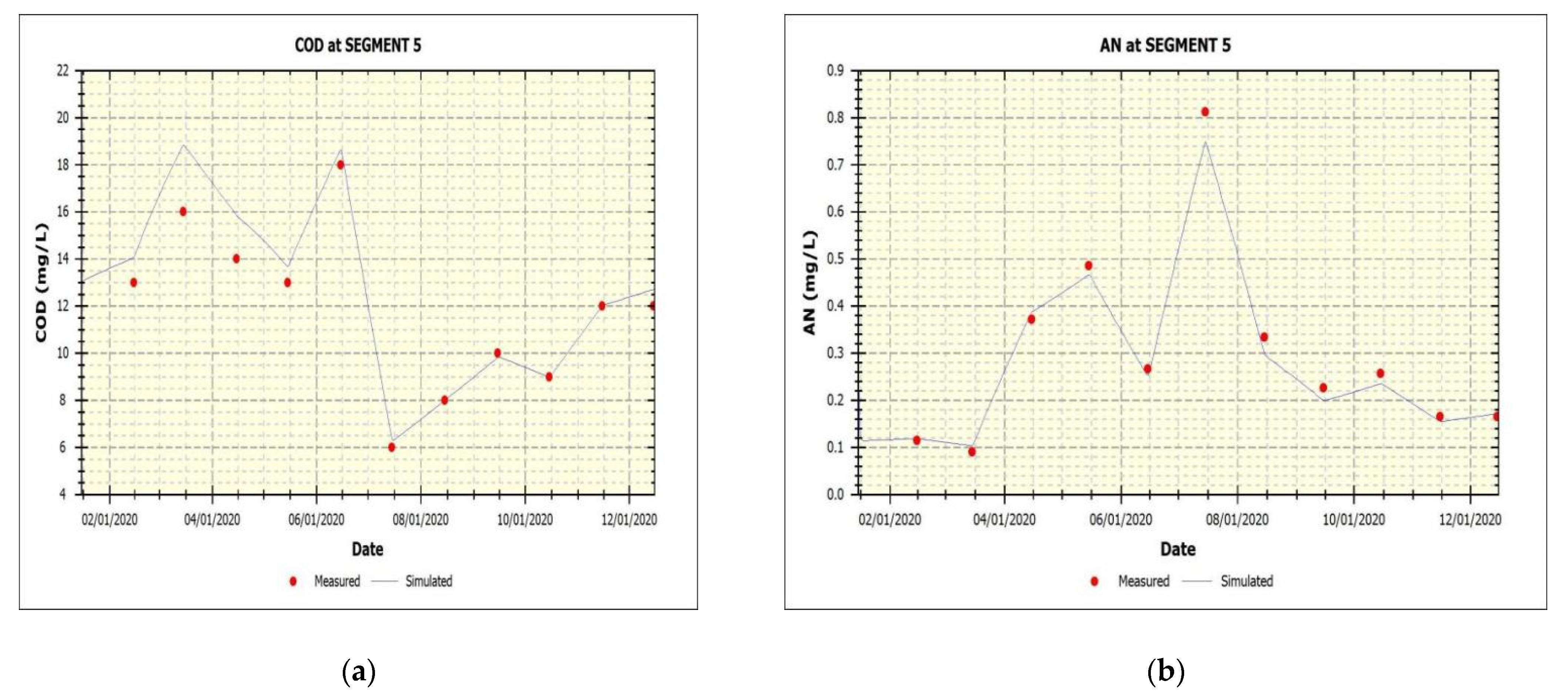
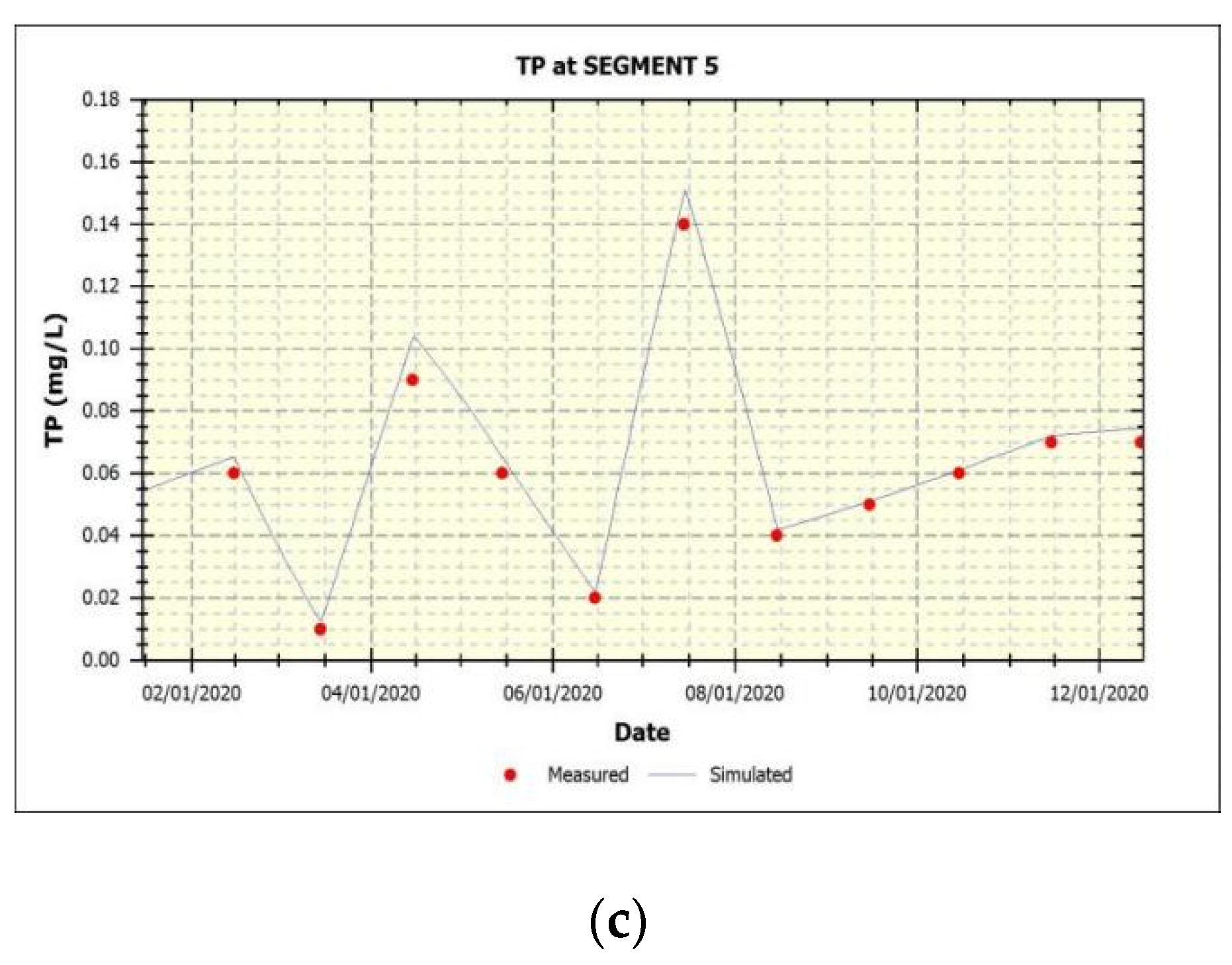
- The analysis of theoretical and optimal parameters: in parameter sensitivity analysis, each initial parameter value is not the fixed value of the parameter. Consequently, the primary purpose of the combined analysis is to find the parameter combination that is closest to the monitored value as the initial combination of parameter rate timing, by improving the efficiency of parameter calibration. For example, the annual average values of the monitoring concentrations of COD, AN, and TP in Segment 5 in 2019 were 13.33 mg/L, 0.18 mg/L, and 0.0525 mg/L, respectively. The concentrations were compared with the output simulated value, and the closer monitoring value was the corresponding parameter combination. At that point it was considered to be the theoretical optimal parameter combination. After comparison, the theoretical optimal combination of COD, AN, and TP was determined, as shown in Table 7.
2.5.2. Calibration of Parameters
2.5.3. Model Verification and Model Accuracy Evaluation
- Model verification:
- Model Accuracy Evaluation:
2.6. Water Environment Capacity
- Water quality aims were to determine the base level of the water environmental management conditions of the Lushui River. Due to the water environmental assessment conditions of Zhuzhou City, the goal of present environmental work in Zhuzhou to upgrade the water quality of the Lushui River to Grade II standard. Water quality standards [30,31] are shown in Table 9.
- To obtain various pollutant environmental capacities and simulate the pollution loads of Lushui River, we determined the water quality requirements for water quality control in the Lushui River basin as the aims of the simulation, and adjusted the input pollution loads of each indicator, such as COD, TP and AN.
- The water quality of the Lushui River was set to Grade II to obtain the water environmental capacity of the Lushui River, and we also considered the pollutants discharged into the Lushui River from both shores.
3. Results
3.1. Parameter Sensitivity Analysis
- For AN: only Θ12 was high sensitivity, K12 was medium sensitivity, and the sensitivity of the remaining parameters were small to negligible;
- For COD: Θd was high sensitivity, Kd was medium sensitivity, and the sensitivity of the remaining parameters were small to negligible;
- For TP: Θ12 was very high sensitivity, Θ83 was high sensitivity, K83 was medium sensitivity, and the sensitivity of the other parameters was small to negligible.
3.2. Model Calibration
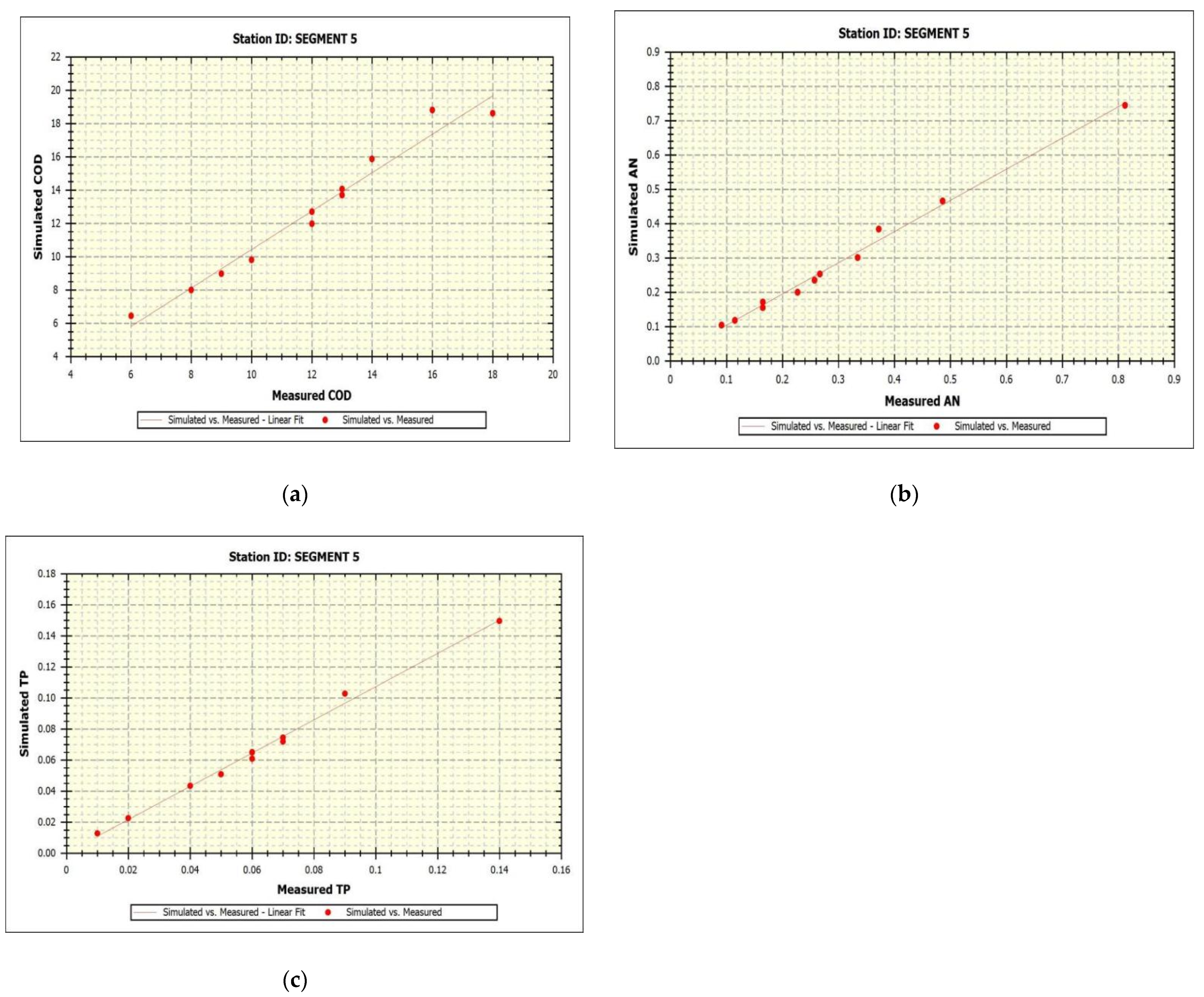
3.3. Simulation Results
3.4. Water Environment Capacity
4. Discussion
4.1. Generalization and Polltion Load
4.2. Parameter Sensitivity Analysis
4.3. Simulation Results and Model Verification
4.4. Model Verification and Model Accuracy Evaluation
4.5. Water Environmental Capacity
5. Conclusions
Author Contributions
Funding
Institutional Review Board Statement
Informed Consent Statement
Data Availability Statement
Acknowledgments
Conflicts of Interest
References
- Fonseca, B.M.; De Mendonça-Galvão, L.; Padovesi-Fonseca, C. Nutrient baselines of Cerrado low-order streams: Comparing natural and impacted sites in Central Brazil. Environ. Monit. Assess. 2014, 186, 19. [Google Scholar] [CrossRef]
- Brooks, B.W.; Riley, T.M.; Taylor, R.D. Water quality of effluent-dominated ecosystems: Ecotoxicological, hydrological, and management considerations. Hydrobiologia 2006, 556, 365–379. [Google Scholar] [CrossRef]
- Zhang, M.L.; Shen, Y.M.; Guo, Y. Development and application of an eutrophication water quality model for river networks. Hydrodynamics 2008, 20, 719–726. [Google Scholar] [CrossRef]
- Ellina, G.; Papaschinopoulos, G.; Papadopoulos, B.K. Research of fuzzy implications via fuzzy linear regression in data analysis for a fuzzy model. J. Comput. Methods Sci. Eng. 2020, 20, 879–888. [Google Scholar] [CrossRef]
- Hu, X. Research on Water Quality Management of Xiangtan Section of Yangtze River Based on WASP Model; Xiangtan University: Xiangtan, China, 2013. (In Chinese) [Google Scholar]
- Lin, J.; Huang, J.-L.; Du, P.-F.; Tu, Z.-S.; Li, Q.-S. Local sensitivity and stability analysis of parameters in urban rainfall runoff hydrological simulation. Environ. Sci. 2010, 31, 2023–2028. [Google Scholar]
- Moriasi, D.N.; Gitau, M.W.; Pai, N.; Daggupati, P. Hydrologic and Water Quality Models: Performance Measures and Evaluation Criteria. Trans. ASABE 2015, 58, 1763–1785. [Google Scholar]
- American Public Health Association; American Water Works Association. Standard Methods for the Examination of Water and Wastewater, 14th ed.; Method 508; American Public Health Association (APHA): Washington, DC, USA, 1975; p. 550. [Google Scholar]
- Ma, L.; Adornato, R.H.; Byrne, D. Yuan Determination of nanomolar levels of nutrients in seawater. Trends Anal. Chem. 2014, 60, 1–15. [Google Scholar] [CrossRef]
- Elser, J.J. Phosphorus: A limiting nutrient for humanity? Curr. Opin. Biotechnol. 2012, 23, 833–838. [Google Scholar] [CrossRef]
- H Šraj, L.O.; Almeida, M.I.G.S.; Swearer, S.E.; Kolev, S.D.; McKelvie, I.D. Analytical challenges and advantages of using flow-based methodologies for ammonia determination in estuarine and marine waters. Trends Anal. Chem. 2014, 59, 83–92. [Google Scholar] [CrossRef]
- Standard. Surface Water Environmental Quality Standard (GB3838-2002); Ministry of Environmental Protection of the People’s Republic of China: Beijing, China, 2002. (In Chinese)
- Seo, I.W.; Baek, K.O. Estimation of the Longitudinal Dispersion Coefficient Using the Velocity Profile in Natural Streams. J. Hydraul. Eng. 2004, 130, 227–236. [Google Scholar] [CrossRef]
- Wijaya, D.S.; Juwan, I. Identification and Calculation of Pollutant Load in Ciwaringin Watershed, Indonesia: Domestic Sector and Faculty of Civil Engineering and Planning; Insttitut Teknologi Nasional Bandung: West Java, Indonesia, 2017. [Google Scholar]
- Xiao, K.X.; Wei, Y.; Ke-feng, L. Estimation and discussion of non-point source pollution loads with new Flux method in Danjiangkou Reservoir area, China. 2016. Available online: https://www.researchgate.net/publication/317291492_Estimation_and_discussion_of_non-point_source_pollution_loads_with_new_Flux_method_in_Danjiangkou_Reservoir_area_China (accessed on 5 October 2021).
- Gu, L.; Hua, Z. Research progress in determining the longitudinal dispersion coefficient of natural rivers. Adv. Sci. Technol. Water Resour. Hydropower 2007, 27, 85–89. [Google Scholar]
- Fischer, H.B. Discussion of Simple Method for Predicting Dispersion in Streams. Keefer. J. Environ. Eng. Div. 1975, 101, 453–455. [Google Scholar] [CrossRef]
- Mcquivey, R.S.; Keefer, T.N. Simple method for predicting dispersion in streams. J. Environ. Eng. Div. 1974, 100, 997–1011. [Google Scholar] [CrossRef]
- Tufford, D.L.; McKellar, H.N. Spatial and temporal hydrodynamic and water quality Modelling analysis of a large reservoir on the South Carolina (USA) coastal plain. Ecol. Model. 1999, 114, 137–173. [Google Scholar] [CrossRef]
- Bae, S.; Seo, D. Analysis and modelling of algal blooms in the Nakdong River. Korea Ecol. Model 2018, 372, 53–63. [Google Scholar] [CrossRef]
- Lenhart, T.; Eckhardt, K.; Fohrer, N. Comparison of two different approaches of sensitivity analysis. Phys. Chem. Earth 2002, 27, 645–654. [Google Scholar] [CrossRef]
- Francos, A.; Elorza, F.J.; Bouraoui, F. Sensitivity analysis of distributed environmental simulation models: Understanding the model behaviour in hydrological studies at the catchment scale. Reliab. Eng. Syst. Saf. 2003, 79, 205–218. [Google Scholar] [CrossRef]
- Peng, S. Research on Uncertainty Water Quality Model Based on WASP Model; Tianjin University: Tianjin, China, 2010. (In Chinese) [Google Scholar]
- Allen, J.I.; Holt, J.T.; Blackford, J.; Proctor, R. Error quantification of a high-resolution coupled hydrodynamic-ecosystem coastal-ocean model: Part 2. Chlorophyll-a, nutrients and SPM. Mar. Syst. 2007, 68, 381–404. [Google Scholar]
- Guo, X.; Yan, S. Sensitivity analysis of rigid pile composite foundation model parameters based on orthogonal design method. J. Self -Sci. Xiangtan Univ. 2015, 37, 15–20. [Google Scholar]
- Cerny, V. Thermodynamical approach to the traveling salesman problem: An efficient simulation algorithm. Optimiz. Theory App. 1985, 45, 41–51. [Google Scholar] [CrossRef]
- Putnam, H. Trial and error predicates and the solution to a problem of Mostowski. Symb. Logic. 1965, 30, 49–57. [Google Scholar] [CrossRef]
- Refsgaard, J.C.; Knudsen, J. Operational validation and intercomparison of different types of hydrological models. Water Resour. Res. 1996, 32, 2189–2202. [Google Scholar] [CrossRef]
- Liu, X. The Heavy Metal Water Quality Target Management Research on Yangtze River Based on Human Health Risk; Central South University: Changsha, China, 2017. (In Chinese) [Google Scholar]
- Sin, G.; de Pauw, D.J.W.; Weijers, S.; Vanrolleghem, P.A. An efficient approach to automate the manual trial and error calibration of activated sludge models. Biotechnol. Bioeng. 2008, 100, 516–528. [Google Scholar] [CrossRef]
- Nash, J.E.; Sutcliffe, J.V. River flow forecasting through conceptual models part I—A discussion of principles. Hydrology 1970, 10, 282–290. [Google Scholar] [CrossRef]


| Segment | Volume | Velocity Mult | Depth Mult | Length | Width | Slope | Bottom Rough |
| 1 | 9.43 × 10⁵ | 1.05 | 1 | 2.21 × 10⁴ | 42.74 | 9.97 × 10⁴ | 0.03 |
| 2 | 9.94 × 10⁵ | 1.26 | 1.5 | 1.20 × 10⁴ | 55.42 | 8.36 × 10⁴ | 0.03 |
| 3 | 4.72 × 10⁶ | 0.89 | 2 | 3.18 × 14 | 74.17 | 2.82 × 10⁴ | 0.03 |
| 4 | 3.18 × 10⁶ | 1.55 | 3 | 1.20 × 10⁴ | 88.47 | 5.01 × 10⁴ | 0.03 |
| 5 | 1.51 × 10⁶ | 0.98 | 1 | 5.46 × 10⁴ | 27.61 | 8.60 × 10⁴ | 0.03 |
| 6 | 1.82 × 10⁶ | 1.04 | 1.3 | 3.79 × 10⁴ | 36.99 | 6.85 × 10⁴ | 0.03 |
| Segment | COD | AN | TP |
|---|---|---|---|
| Segment 1 | 26769.6 | 1031.616 | 277.416 |
| Segment 2 | 29318.4 | 1226.751 | 305.424 |
| Segment 3 | 22910.4 | 359.452 | 187.704 |
| Segment 4 | 210024 | 6440.76 | 2496.268 |
| Segment 5 | 28687.68 | 681.883 | 140.112 |
| Segment 6 | 26618.4 | 506.800 | 124.56 |
| Segments | COD | AN | TP |
|---|---|---|---|
| Segment 1 | 46656 | 747.468 | 226.8 |
| Segment 2 | 42026.4 | 706.176 | 153.216 |
| Segment 3 | 25934.4 | 301.176 | 261.432 |
| Segment 4 | 286387.2 | 4972.032 | 2865.384 |
| Segment 5 | 28296 | 427.104 | 110.664 |
| Segment 6 | 24429.6 | 361.44 | 78.192 |
| Segments | EX | Segments | EX |
|---|---|---|---|
| Segment 1 | 43.047 | Segment 4 | 405.725 |
| Segment 2 | 48.939 | Segment 5 | 62.246 |
| Segment 3 | 79.564 | Segment 6 | 53.134 |
| Boundary | COD (mg/L) | AN (mg/L) | TP (mg/L) |
|---|---|---|---|
| Segment 1 | 13.5 | 0.284 | 0.09 |
| Segment 4 | 10 | 0.12 | 0.1 |
| Segment 5 | 13 | 0.31 | 0.06 |
| Sensitivity Index | Grading Standard | Level |
|---|---|---|
| 0.00 ≤ SS ≤ 0.05 | Small to negligible | 1 |
| 0.05 ≤ SS ≤ 0.20 | Medium | 2 |
| 0.20 ≤ Ss ≤ 1.00 | High | 3 |
| Ss ≥ 1.00 | Very high | 4 |
| K12 | Θ12 | K83 | Θ83 | Kd | Θd |
|---|---|---|---|---|---|
| 0.0972 | 0.832 | 0.144 | 0.856 | 0.2772 | 0.8376 |
| Measure | Coefficient of Determination | Performance Rating |
|---|---|---|
| 0.00 ≤ R2 ≤0.40 | Unsatisfactory | |
| R2 | 0.40 ≤ R2 ≤ 0.60 | Satisfactory |
| 0.60 ≤ R2 ≤ 0.75 | Good | |
| 0.75 ≤ R2 ≤ 1 | Very Good |
| Indicators | I | II | III | IV |
| COD | 15 | 15 | 20 | 30 |
| AN | 0.15 | 0.5 | 1.0 | 1.5 |
| TP | 0.02 | 0.1 | 0.2 | 0.3 |
| Symbol | COD | AN | TP | |||||||||
|---|---|---|---|---|---|---|---|---|---|---|---|---|
| (−50%) | (+50%) | SS | Class | (−50%) | (+50%) | SS | Class | (−50%) | (+50%) | SS | Class | |
| K12 * | 0 | 0.000 | 0.000 | 1 | 0.025 * | 0.075 * | 0.05 * | 2 * | 0 | 0 | 0 | 1 |
| Θ12 * | 0 | 0.000 | 0.000 | 1 | 0.369 * | 0.387 * | 0.378 * | 3 * | 0 | 2.062 * | 1.031 * | 4 * |
| KNO3 | 0 | 0.000 | 0.000 | 1 | 0.001 | 0.003 | 0.002 | 1 | 0 | 0 | 0 | 1 |
| Tmin | 0 | 0.000 | 0.000 | 1 | 0 | 0 | 0 | 1 | 0 | 0 | 0 | 1 |
| K2D | 0 | 0.000 | 0.000 | 1 | 0 | 0 | 0 | 1 | 0 | 0 | 0 | 1 |
| Θ2D | 0 | 0.000 | 0.000 | 1 | 0 | 0 | 0 | 1 | 0 | 0 | 0 | 1 |
| KNO3 | 0.000 | 0.000 | 0.000 | 1 | 0 | 0 | 0 | 1 | 0 | 0 | 0 | 1 |
| K71 | 0.000 | 0.000 | 0.000 | 1 | 0 | 0 | 0 | 1 | 0 | 0 | 0 | 1 |
| K83 * | 0.000 | 0.000 | 0.000 | 1 | 0 | 0 | 0 | 1 | 0 | 0.111 * | 0.055 * | 2 * |
| Θ71 | 0.000 | 0.000 | 0.000 | 1 | 0 | 0 | 0 | 1 | 0 | 0 | 0 | 1 |
| Θ83 * | 0.000 | 0.000 | 0.000 | 1 | 0 | 0 | 0 | 1 | 0.44 * | 0.413 * | 0.427 * | 3 * |
| Kd * | 0.065 * | 0.196 * | 0.131 * | 2 * | 0 | 0 | 0 | 1 | 0 | 0 | 0 | 1 |
| Θd * | 0.319 * | 0.612 * | 0.465 * | 3 * | 0 | 0 | 0 | 1 | 0 | 0 | 0 | 1 |
| KCOD | 0.003 | 0.009 | 0.006 | 1 | 0 | 0 | 0 | 1 | 0 | 0 | 0 | 1 |
| fD5 | 0.000 | 0.000 | 0.000 | 1 | 0 | 0 | 0 | 1 | 0 | 0 | 0 | 1 |
| R | 0.000 | 0.000 | 0.000 | 1 | 0 | 0 | 0 | 1 | 0 | 0 | 0 | 1 |
| Parameter Name | Symbol | Value | Unit |
|---|---|---|---|
| Nitrification Rate Constant at 20 °C | K12 | 0.081 | d−1 |
| Nitrification Temperature Coefficient | Θ12 | 1.04 | |
| Half Saturation Constant for Nitrification Oxygen Limit | KNO3 | 0.5 | mgO2/L |
| Minimum Temperature for Nitrification Reaction | Tmin | 3 | °C |
| Denitrification Rate Constant at 20 °C | K2D | 0.045 | d−1 |
| Denitrification Temperature Coefficient | Θ2D | 1.04 | |
| Half Saturation Constant for Denitrification Oxygen Limit | KNO3 | 0.1 | mgO2/L |
| Dissolved Organic Nitrogen Mineralization Rate Constant at 20 °C | K71 | 0.075 | d−1 |
| Dissolved Organic Phosphorus Mineralization Rate Constant at 20 °C | K83 | 0.12 | d−1 |
| Dissolved Organic Nitrogen Mineralization Temperature Coefficient | Θ71 | 1.08 | |
| Dissolved Organic Phosphorus Mineralization Temperature Coefficient | Θ83 | 1.07 | |
| COD Decay Rate Constant at 20 °C | Kd | 0.231 | d−1 |
| COD Decay Rate Temperature Correction Coefficient | Θd | 1.047 | |
| COD Half Saturation Oxygen Limit | KCOD | 0.5 | mgO2/L |
| Fraction of Detritus Dissolution to COD | f D5 | 0.2 | |
| Fraction of COD Carbon Source for Denitrification | R | 0.2 |
| Segments | COD | AN | TP | ||||||
|---|---|---|---|---|---|---|---|---|---|
| Normal | Wet | Dry | Normal | Wet | Dry | Normal | Wet | Dry | |
| Segment 1 | 8.837 | 5.223 | 8.654 | 0.392 | 0.314 | 0.418 | 0.130 | 0.097 | 0.105 |
| Segment 2 | 19.140 | 9.468 | 13.320 | 0.731 | 0.469 | 0.795 | 0.191 | 0.160 | 0.195 |
| Segment 3 | 12.376 | 7.732 | 9.623 | 0.325 | 0.243 | 0.325 | 0.095 | 0.092 | 0.110 |
| Segment 4 | 38.393 | 44.830 | 38.922 | 1.355 | 1.258 | 0.844 | 0.425 | 0.645 | 0.290 |
| Segment 5 | 15.609 | 10.697 | 11.671 | 0.269 | 0.374 | 0.218 | 0.061 | 0.067 | 0.067 |
| Segment 6 | 16.141 | 10.712 | 10.229 | 0.263 | 0.373 | 0.157 | 0.071 | 0.068 | 0.063 |
| Segments | COD | AN | TP | ||||||
|---|---|---|---|---|---|---|---|---|---|
| Normal | Wet | Dry | Normal | Wet | Dry | Normal | Wet | Dry | |
| Segment 1 | 14,072.94 | 17,147.7 | 10,998.18 | 469.098 | 571.59 | 366.606 | 93.8196 | 114.318 | 73.3212 |
| Segment 2 | 21,286.8 | 19,512.9 | 17,975.52 | 709.56 | 650.43 | 599.184 | 141.912 | 130.086 | 119.8368 |
| Segment 3 | 13,481.64 | 14,427.72 | 11,944.26 | 449.388 | 480.924 | 398.142 | 89.8776 | 96.1848 | 79.6284 |
| Segment 4 | 135,525.96 | 185,195.16 | 85,738.5 | 4517.532 | 6173.17 | 2857.95 | 903.5064 | 1234.634 | 571.59 |
| Segment 5 | 15,846.84 | 12,417.3 | 10,288.62 | 528.228 | 413.91 | 342.954 | 105.6456 | 82.782 | 68.5908 |
| Segment 6 | 12,949.47 | 12,831.21 | 7686.9 | 431.649 | 427.707 | 256.23 | 86.3298 | 85.5414 | 51.246 |
| Total | 14,072.94 | 17,147.7 | 10,998.18 | 469.098 | 571.59 | 366.606 | 93.8196 | 114.318 | 73.3212 |
| Date (MM/DD/YY) | COD | AN | TP | ||||||
|---|---|---|---|---|---|---|---|---|---|
| Simulated | Observed | f | Simulated | Observed | f | Simulated | Observed | f | |
| 1/15/2020 | 13.000 | 12 | 8.33% | 0.115 | 0.107 | 7.04% | 0.055 | 0.05 | 9.79% |
| 2/15/2020 | 14.083 | 13 | 8.33% | 0.118 | 0.115 | 2.98% | 0.065 | 0.06 | 8.25% |
| 3/15/2020 | 18.842 | 16 | 17.76% | 0.105 | 0.091 | 15.09% | 0.012 | 0.01 | 24.86% |
| 4/15/2020 | 15.831 | 14 | 13.08% | 0.387 | 0.372 | 4.02% | 0.104 | 0.09 | 15.23% |
| 5/15/2020 | 13.682 | 13 | 5.25% | 0.466 | 0.486 | 4.12% | 0.065 | 0.06 | 7.54% |
| 6/15/2020 | 18.629 | 18 | 3.50% | 0.252 | 0.267 | 5.46% | 0.022 | 0.02 | 11.65% |
| 7/15/2020 | 6.313 | 6 | 5.21% | 0.749 | 0.812 | 7.82% | 0.151 | 0.14 | 7.73% |
| 8/15/2020 | 8.019 | 8 | 0.24% | 0.296 | 0.334 | 11.40% | 0.042 | 0.04 | 5.63% |
| 9/15/2020 | 9.828 | 10 | 1.72% | 0.199 | 0.227 | 12.38% | 0.051 | 0.05 | 2.11% |
| 10/15/2020 | 8.979 | 9 | 0.24% | 0.235 | 0.257 | 8.50% | 0.061 | 0.06 | 1.67% |
| 11/15/2020 | 12.007 | 11.8 | 1.76% | 0.155 | 0.165 | 6.31% | 0.072 | 0.07 | 2.88% |
| 12/15/2020 | 12.700 | 11.8 | 7.62% | 0.171 | 0.165 | 3.90% | 0.074 | 0.07 | 6.31% |
| COD | AN | TP | ||||
|---|---|---|---|---|---|---|
| Statistics | Measured | Simulated | Measured | Simulated | Measured | Simulated |
| Count | 12 | 12 | 12 | 12 | 12 | 12 |
| Min | 6.000 | 6.313 | 0.091 | 0.104 | 0.010 | 0.012 |
| Max | 18.000 | 18.842 | 0.812 | 0.749 | 0.140 | 0.151 |
| Coef of Det (R2) | 0.97 | 0.99 | 0.99 | |||
| Mean Abs Error | 0.764 | 0.021 | 0.004 | |||
| RMS Error | 1.129 | 0.027 | 0.006 | |||
| Norm RMS Error | 0.088 | 0.078 | 0.079 | |||
| Index of Agreement (r) | 0.98 | 0.99 | 0.99 |
Publisher’s Note: MDPI stays neutral with regard to jurisdictional claims in published maps and institutional affiliations. |
© 2021 by the authors. Licensee MDPI, Basel, Switzerland. This article is an open access article distributed under the terms and conditions of the Creative Commons Attribution (CC BY) license (https://creativecommons.org/licenses/by/4.0/).
Share and Cite
Obin, N.; Tao, H.; Ge, F.; Liu, X. Research on Water Quality Simulation and Water Environmental Capacity in Lushui River Based on WASP Model. Water 2021, 13, 2819. https://doi.org/10.3390/w13202819
Obin N, Tao H, Ge F, Liu X. Research on Water Quality Simulation and Water Environmental Capacity in Lushui River Based on WASP Model. Water. 2021; 13(20):2819. https://doi.org/10.3390/w13202819
Chicago/Turabian StyleObin, Nicolas, Hongni Tao, Fei Ge, and Xingwang Liu. 2021. "Research on Water Quality Simulation and Water Environmental Capacity in Lushui River Based on WASP Model" Water 13, no. 20: 2819. https://doi.org/10.3390/w13202819
APA StyleObin, N., Tao, H., Ge, F., & Liu, X. (2021). Research on Water Quality Simulation and Water Environmental Capacity in Lushui River Based on WASP Model. Water, 13(20), 2819. https://doi.org/10.3390/w13202819