Implications of Experiment Set-Ups for Residential Water End-Use Classification

Abstract

With an increasing need for secured water supply, a better understanding of the water consumption behavior is beneficial. This can be achieved through end-use classification, i.e., identifying end-uses such as toilets, showers or dishwashers from water consumption data. Previously, both supervised and unsupervised machine learning (ML) techniques are employed, demonstrating accurate classification results on particular datasets. However, a comprehensive comparison of ML techniques on a common dataset is still missing. Hence, in this study, we are aiming at a quantitative evaluation of various ML techniques on a common dataset. For this purpose, a stochastic water consumption simulation tool with high capability to model the real-world water consumption pattern is applied to generate residential data. Subsequently, unsupervised clustering methods, such as dynamic time warping, k-means, DBSCAN, OPTICS and Hough transform, are compared to supervised methods based on SVM. The quantitative results demonstrate that supervised approaches are capable to classify common residential end-uses (toilet, shower, faucet, dishwasher, washing machine, bathtub and mixed water-uses) with accuracies up to 0.99, whereas unsupervised methods fail to detect those consumption categories. In conclusion, clustering techniques alone are not suitable to separate end-use categories fully automatically. Hence, accurate labels are essential for the end-use classification of water events, where crowdsourcing and citizen science approaches pose feasible solutions for this purpose.

1. Introduction

In recent years, climate change and population growth have exacerbated water scarcity and accelerated the vulnerability of water supply systems. A comprehensive and detailed understanding of water demand as well as water end-uses will improve the resilience of these systems. With the water consumption data generated and transmitted by smart water meters, advanced analysis of water demand using data-driven approaches is facilitated. In particular, the categorization of water use events into residential end-uses like washing machine, faucet or toilet permits a detailed investigation of the impact of different end-uses as well as the inhabitants on the overall demand. With the recent advances in artificial intelligence, categorization of residential water end-use can be resolved as classification problem using Machine Learning (ML) techniques, thus having inherent real-time capability, scalability and generalizability. On a basic level, ML techniques can be subdivided into supervised and unsupervised approaches. The former directly perform a categorization/classification of data with given categories. Consequently, training data with labels annotating the samples’ categories are necessary. The latter search for groups of similar data points in the dataset in the absence of labels.

Both unsupervised and supervised approaches are widely applied in studies on end-use classifications of water use events. For example, Pastor-Jabaloyes et al. [1] proposed an unsupervised approach formulating a Partition Around Medoids clustering method using Gower distance as a similarity measure in the feature space, which is spanned by the volume and the average flow rate of the water use events. A clustering algorithm based on Dynamic Time Warping (DTW) as the similarity measure between events is described by Nguyen et al. [2]. This algorithm was refined to a hybrid method comprising k-medoids clustering, DTW and a swarm-intelligence-based global optimization, i.e., Artificial Bee Colony algorithm. Later, this approach was extended with a hybrid method consisting of Self-Organizing Maps and a k-means algorithm in the subsequent publications [3,4]. Most supervised approaches are based on Hidden Markov Models and a subsequent optimization [5,6,7,8,9,10,11,12,13,14,15,16], but Artificial Neural Networks [9,10,11,12,13], Decision Trees [14] and Multi-category Robust Linear Programming [17] are used as well. Support Vector Machines (SVMs) were employed by Vitter et al. [18] to categorize water events using water consumption data and coincident electricity data. Furthermore, Carranza et al. [19] identified residential water end-uses in data measured by precision water meters equipped with pulse emitters using SVMs.

Both supervised and unsupervised approaches proposed in the literature demonstrate high performance in terms of accuracy with the particular dataset utilized in corresponding experiments. However, these datasets are often acquired in different countries or regions. Consequently, the underlying consumer behavior represented by the consumption data varies. Moreover, each dataset has a specific time resolution. Thus, the characteristic of the datasets utilized in the state-of-the-art literature differs largely. As the methods proposed in the aforementioned studies are mainly customized to the particular dataset, the generalizability of each method is not proven. Moreover, the particular datasets applied in the state-of-the-arts are commonly not publicly available. Hence, the corresponding implementation (e.g., setting of model hyperparameters) of the proposed ML models is not traceable. This results in a decreased reproducibility of the methods. Finally, to the best of our knowledge a comprehensive comparison of both supervised and unsupervised approaches on a common database has not been performed yet.

In this paper, we focus on a comparative evaluation of supervised and unsupervised ML techniques on a common dataset for the application of residential water end-use classification and aim at deriving a decision support for the selection of the appropriate approach, revealing possible pitfalls of water end-use classification. For this purpose, we implemented a large variety of ML-based approaches proposed in the state-of-the-art literature, i.e., the clustering algorithm based on DTW established by Nguyen et al. [2], k-means, Density-Based Spatial Clustering of Applications with Noise (DBSCAN), Ordering Points To Identify the Clustering Structure (OPTICS), Clustering in Arbitrary Subspaces based on the Hough transform (CASH), as well as two classifiers based on Support Vector Machines (SVM). Subsequently, the methods are evaluated on a common database generated using a stochastic water consumption simulation framework. The validation of different algorithms with a common dataset guarantees the comparability of the evaluation results. Finally, evaluation results are analyzed and discussed in detail, with the intention to draw implications and recommendations of experiment set-ups for data-driven water end-use classification in general.

2. Methods

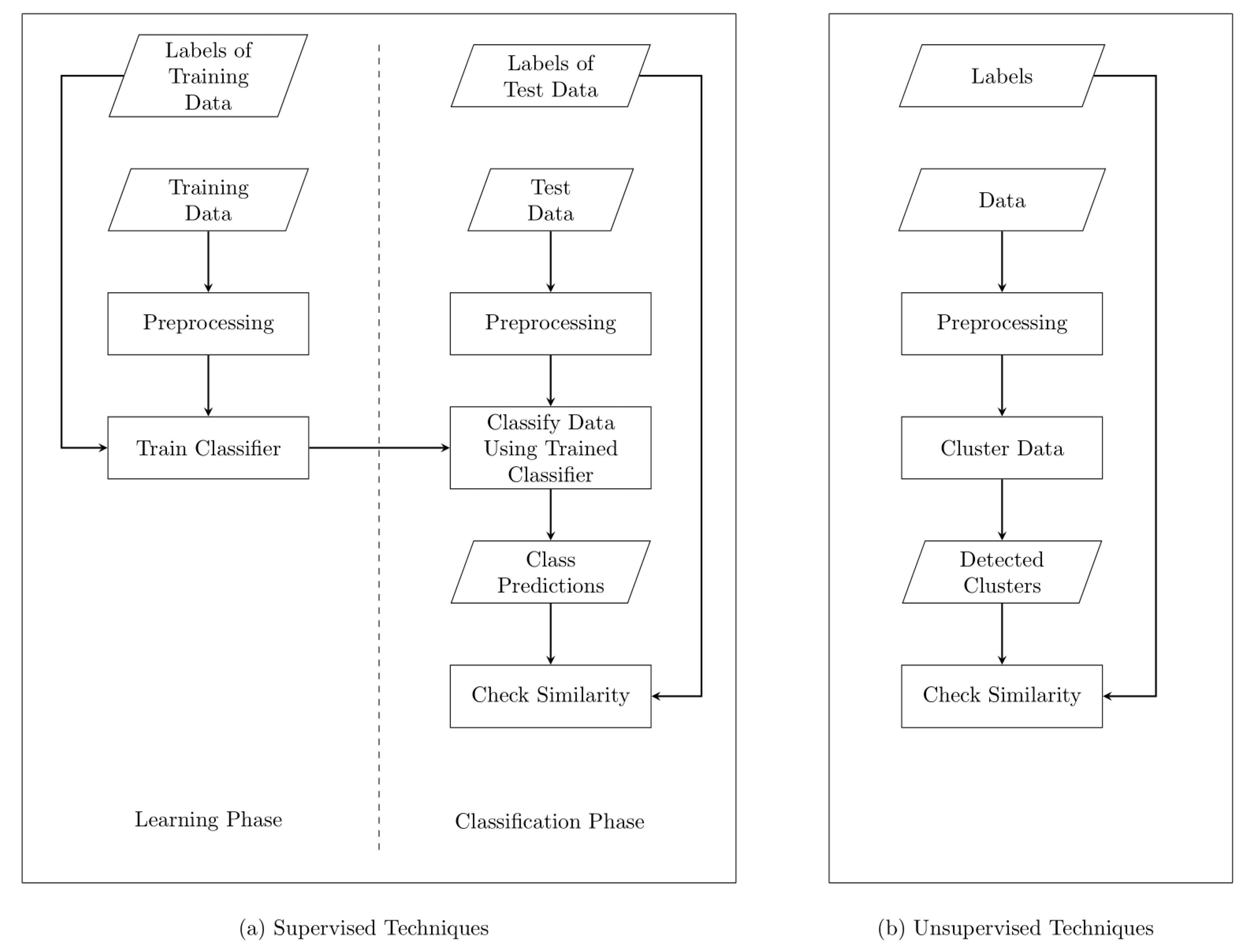
In this section, the simulated common water consumption database as well as the ML techniques employed and evaluated in this work are described in detail. An overview of supervised and unsupervised ML methods is presented in Figure 1. For the supervised methods as well as the clustering algorithms k-means, DBSCAN and OPTICS, the open-source library scikit-learn [20] is used. The clustering algorithm based on DTW is implemented after Nguyen et al. [2], and the open-source data mining framework ELKI [21] provides the clustering algorithm CASH. Both labels and water consumption data are generated with a stochastic simulation proposed in [16].

2.1. Simulation of Common Database and Data Preprocessing

The datasets employed in this paper are generated using the STochastic Residential water End-use Model (STREaM) developed by Cominola et al. [16]. It is a stochastic water consumption simulation tool with a high capability to model the real-world water consumption patterns of the end-uses, such as toilet, shower, faucet, dishwasher, washing machine and bathtub. STREaM is calibrated using observed and disaggregated water consumption data from 300 single-family houses in nine U.S. cities. With a stochastic model based on Monte Carlo simulation, time series with different temporal resolutions (up to 10 s) and number of inhabitants can be emulated. To the best of our knowledge, STREaM is the most advanced framework for realistic water consumption simulation to date.

In this work, the chosen temporal resolution is ten seconds, which corresponds to the highest possible resolution of the simulation tool. Six datasets are generated with a varying number of inhabitants from one to six. In addition to the resolution and the number of inhabitants, the efficiency of the present end-uses and the time horizon of the datasets are fixed to “standard fixture” (i.e., fixtures which are not specified to improve the water use efficiency) and one year, respectively. These datasets are publicly available (see supplementary materials).

The output of the simulation includes six time series corresponding to the end-use toilet, shower, faucet, washing machine, dishwasher and bathtub. An additional time series aggregating the six above mentioned end-uses is also generated. The entire aggregated time series is segmented into water use events (or sequences) with the assumption that a contiguous water consumption event does not have any interruption which is longer than 150 s. Since the timestamps of each event are known, labels for events extracted from the aggregated time series are computed by searching for water consumption at these timestamps in the time series representing the single end-uses. The result of the preprocessing is a set of water use event time series with corresponding end-use labels. Events with a consumption of less or equal to one liter as well as events with more than 1000 L are removed from this set, as they indicate leaks and might not be connected to an end-use of interest.

2.2. Feature Description and Feature Extraction

Prior to the application of classification or clustering techniques, relevant features describing the water events are commonly selected from the simulated water consumption data, except for a DTW based algorithm described in Section 2.4.1. Features selected in this work include volume, duration, maximum, minimum and most common flow rate, as well as the corresponding numbers of occurrences of these flow rates, the number of different flow rates and two orthogonal harmonic functions representing the time of the day. Since these features have different scales, we performed z-normalization in order to prevent the effect that features with a larger scale will dominate the other. Subsequently, we compute the pair-wise Pearson Correlation Coefficient (PCC) of the features, and exclude one of the two features when the PCC is higher than 0.9. In order to deal with the curse of dimensionality, Principal Component Analysis is employed as dimensionality reduction technique prior to all algorithms except for CASH (refer to Section 2.4.5).

2.3. Supervised Techniques

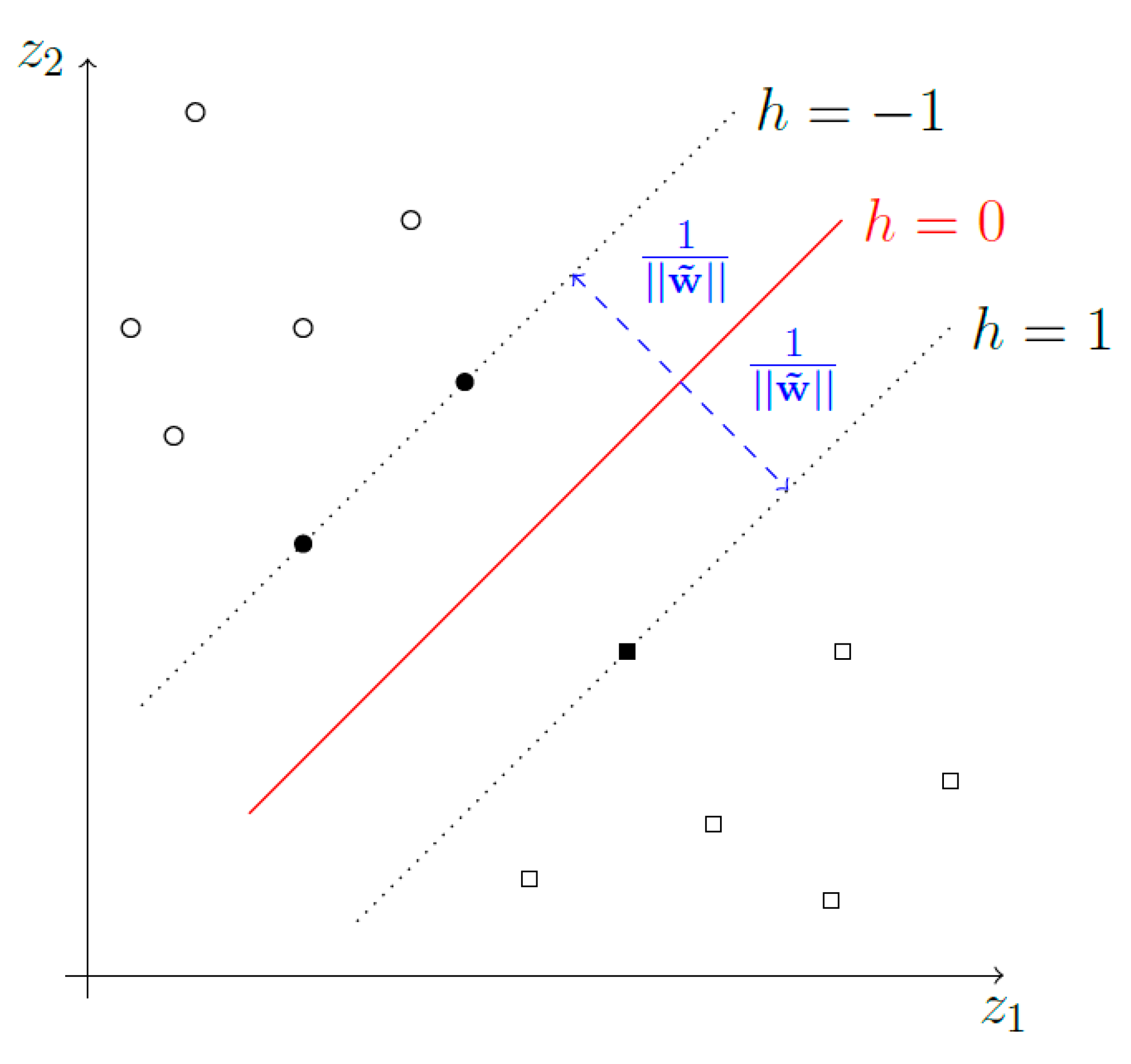
In the category supervised learning techniques, we implemented two classifiers, namely a multi-class SVM as well as binary SVMs per end-use. Generally, SVMs [22] separate classes with a maximal margin hyperplane in the feature space as depicted in Figure 2. In a linearly separable problem, the data points (i.e., feature vectors) on the margin boundaries are called support vectors. Considering a real-world binary (or two-class) classification problem, the two classes are not perfectly linearly separable in practice. Therefore, the support vectors lie within the margin boundaries. The maximal margin hyperplane can be described solely based on the support vectors, making SVMs memory efficient. The location of a new data point with regard to the hyperplane defines the point’s class membership, as the hyperplane separates the two classes in the feature space.

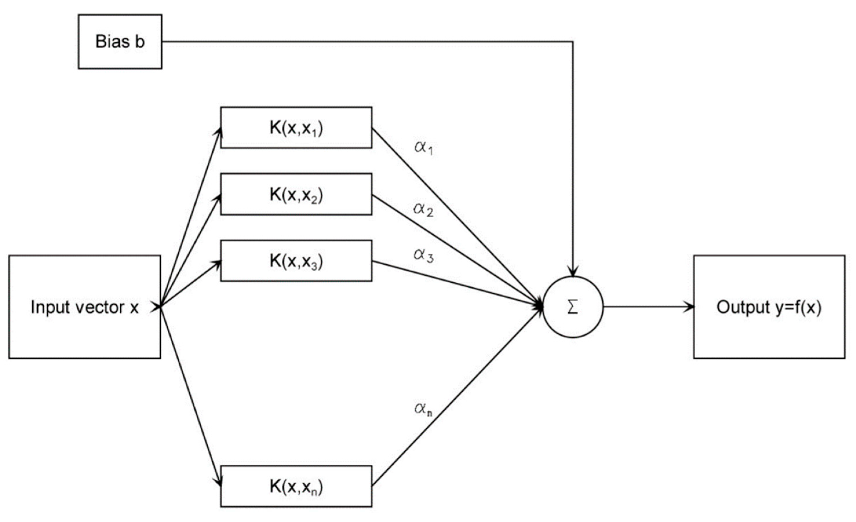
To combat the challenges of non-linear problems, kernel functions are employed to map data points into higher dimensional spaces, where the points are linearly separable. Hence, SVMs show a two-layer structure as described in [23], which employ Support Vector regression to model rainfall-runoff in urban drainage. The two-layer structure is displayed in Figure 3. In the first layer, the non-linear kernel is applied to the support vectors and the input vector. The second layer consists of a weighted sum of the kernel outputs. In contrast to the regression implemented in [23], only the sign of the weighted sum is of relevance for a classification task, as the sign determines the side of the hyperplane on which the input vector lies. Consequently, the sign determines the class membership, as each subspace separated by the hyperplane corresponds to one of the two classes. In our study, the chosen kernel is a Radial Basis Function and the regularization parameters for the SVMs are set to 1.0 for all experiments conducted.

2.4. Unsupervised Techniques

The unsupervised methods evaluated in this paper include the clustering algorithm based on DTW established by Nguyen et al. [2], k-means, DBSCAN, OPTICS and CASH. Each of them is described in detail in the following sections.

2.4.1. Threshold-Based Clustering Using Dynamic Time Warping

The algorithm presented in [2] is based on the idea that the similarity of two events (or sequences) of a time series can be approximated by their distances to a reference event. This reference event is chosen arbitrarily from the dataset as described in [8] and will not be clustered. First, DTW distances of all water use events in the dataset to the reference event are calculated. Subsequently, relative distances are computed for each sequence. A threshold α is introduced to assign the event to a cluster. For algorithmic details, we refer to the original work published in [2]. In this study, the threshold α is manually fine-tuned to 0.6.

2.4.2. K-Means

K-means is one of the most frequently used clustering algorithms, which use Euclidean distances in the feature space (refer to 2.2) to determine cluster memberships. The optimal hyperparameter k, i.e., the number of clusters, is computed with an Elbow method using inertia. The output of this analysis, namely, k = 10, is fixed for all experiments conducted.

2.4.3. DBSCAN

In contrast to k-means, DBSCAN [24] is a density-based clustering algorithm. It uses the concept of core, border and noise points to form partitions in the feature space. Two hyperparameters, eps and minPts, are required to distinguish these three types of points. A neighborhood with a radius of eps around each feature vector is selected, and the number of feature vectors in its neighborhood is counted. If a vector has more than minPts neighbors, then this vector is considered to be a core point. If a vector has less than minPts neighbors but one core point in its neighborhood, then this vector is a border point. All remaining vectors are noise points. The superposition of core and border points forms clusters. Unlike k-means, DBSCAN determines the number of clusters intrinsically based on the distribution of data points in the feature space. minPts and eps are set to 14 and 2, respectively, where the former is calculated with the rule of thumb minPts = 2 · number of dimensions after dimensionality reduction [25], and the latter is estimated with a 14-Nearest Neighbor Distance Graph.

2.4.4. OPTICS

OPTICS [26] is an extended version of DBSCAN, and hence, it also applies the notion of core, border and noise points. However, instead of looking at a fixed neighborhood area, an infinite number of distance parameters eps_i is applied, which are smaller than a “generating distance” eps_max (0 ≤ eps_i ≤ eps_max). This allows OPTICS to find clusters of different densities in the feature space. eps_max can simply be set to infinity, as this will identify clusters across all scales [20]. In the original paper [26], experiments indicated that values between 10 and 20 for minPts will always lead to promising results. Hence, minPts is chosen to be 15 in this work.

2.4.5. CASH

CASH [27] is a clustering algorithm specifically designed for high-dimensional data. It uses a Hough transform to bypass the curse of dimensionality. The feature vectors are transformed from the feature space to a parameter space, which corresponds to the space of all possible subspaces of the feature space. Vectors in the feature space are equivalent to sinusoidal curves in the parameter space. Instead of looking at a spatial proximity in the feature space to form clusters, intersections of curves in the parameter space are determined. An intersection in the parameter space means that the two vectors in the feature space lie on a common hyperplane, therefore are correlated. Since CASH does not rely on any distance-based measures in the feature space, it is not affected by curse of dimensionality. Consequently, dimensionality reduction techniques are dispensable. The three hyperparameters, namely, minimum number of points in a cluster, the maximal allowed deviation and the maximum number of successive splits, are set to 20, 0.1 and 3, respectively.

3. Results and Discussion

The datasets described in Section 2.1 are addressed as 1P, 2P, 3P, 4P, 5P and 6P, referring to the number of inhabitants in the simulated household. The following sections provide the evaluation of the supervised and unsupervised techniques using these six datasets. The employed code is executed with python 3.7, making use of the ELKI version 0.7.5 and the scikit-learn version 0.23.1. ELKI is run with OpenJDK 13.0.33. Upon calling CASH with OpenJDK, 12 GB are allocated for its execution. All experiments were conducted with the same hardware, equipped with an Intel(R) Core(TM) i9-8950HK CPU @ 2.90GHz (6 cores), 16 GB RAM and a 64 bit Windows 10 operating system.

3.1. Evaluation of the Supervised Techniques

For a fair comparison, we calculated accuracy and precision both for multi-class and binary SVMs. In detail, precision, recall and f1-score for all classified end-uses are first estimated for the multi-class SVMs. The accuracy is computed in the subsequent step. For binary SVMs, confusion matrices are used to compute accuracies and precisions of the classifiers, as the number of positive and negative samples is highly unbalanced. The split of training and test data is 0.8 to 0.2 for all experiments conducted.

3.1.1. Evaluation Results

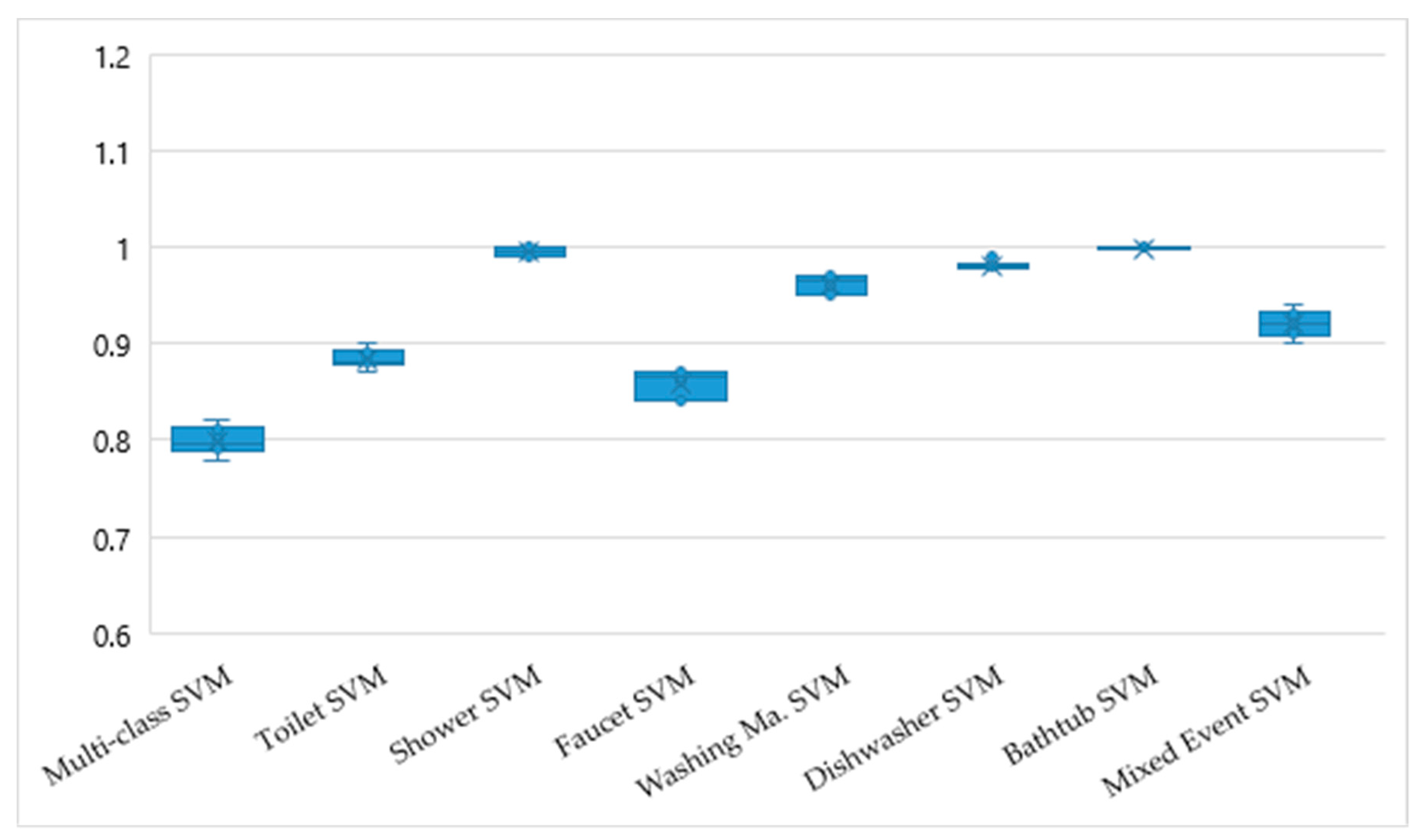
Figure 4 presents the quantitative comparison of the accuracies for multi-class and binary SVMs. The evaluation results for the multi-class SVMs are detailed in

Table A1. Classification report for the 1P dataset.

	Precision	Recall	F1-Score	Support
0 1	0.66	0.63	0.65	150
1 1	0.80	0.84	0.82	466
2 1	0.80	0.96	0.87	49
3 1	0.83	0.89	0.86	775
4 1	0.84	0.56	0.67	137
5 1	0.25	0.02	0.04	47
6 1	0.56	0.56	0.56	9
Accuracy 2			0.80	1633
Macro Average	0.68	0.64	0.64	1633
Weighted Average	0.79	0.80	0.79	1633

¹ The rows in the classification report correspond to the end-use labels: 0 = Overlapping, 1 = Toilet, 2 = Shower, 3 = Faucet, 4 = Washing Machine, 5 = Dishwasher, 6 = Bathtub. ² The micro average corresponds to the accuracy. If only one subset of the classes is present in the predictions for the test data, the two metrics are not equivalent.

,

Table A2. Classification report for the 2P dataset.

	Precision	Recall	F1-Score	Support
0 1	0.69	0.66	0.68	289
1 1	0.79	0.87	0.83	692
2 1	0.89	0.91	0.90	56
3 1	0.85	0.86	0.86	1098
4 1	0.77	0.58	0.66	110
5 1				0
6 1	1.00	0.50	0.67	2
Micro Average	0.81	0.82	0.82	2247
Macro Average	0.83	0.73	0.77	2247
Weighted Average	0.81	0.82	0.82	2247

¹ The rows in the classification report correspond to the end-use labels: 0 = Overlapping, 1 = Toilet, 2 = Shower, 3 = Faucet, 4 = Washing Machine, 5 = Dishwasher, 6 = Bathtub.

,

Table A3. Classification report for the 3P dataset.

	Precision	Recall	F1-Score	Support
0 1	0.69	0.70	0.69	379
1 1	0.77	0.80	0.78	708
2 1	0.87	0.92	0.90	66
3 1	0.81	0.85	0.83	1253
4 1	0.82	0.61	0.70	137
5 1				0
6 1	0.80	0.57	0.67	7
Micro Average	0.78	0.80	0.79	2550
Macro Average	0.79	0.74	0.76	2550
Weighted Average	0.78	0.80	0.79	2550

¹ The rows in the classification report correspond to the end-use labels: 0 = Overlapping, 1 = Toilet, 2 = Shower, 3 = Faucet, 4 = Washing Machine, 5 = Dishwasher, 6 = Bathtub.

,

Table A4. Classification report for the 4P dataset.

	Precision	Recall	F1-Score	Support
0 1	0.78	0.75	0.77	471
1 1	0.79	0.83	0.81	844
2 1	0.95	0.89	0.92	89
3 1	0.82	0.86	0.84	1275
4 1	0.76	0.71	0.73	166
5 1				0
6 1	1.00	0.33	0.50	3
Micro Average	0.81	0.82	0.81	2848
Macro Average	0.85	0.73	0.76	2848
Weighted Average	0.81	0.82	0.81	2848

¹ The rows in the classification report correspond to the end-use labels: 0 = Overlapping, 1 = Toilet, 2 = Shower, 3 = Faucet, 4 = Washing Machine, 5 = Dishwasher, 6 = Bathtub.

,

Table A5. Classification report for the 5P dataset.

	Precision	Recall	F1-Score	Support
0 1	0.70	0.77	0.73	505
1 1	0.77	0.82	0.79	873
2 1	0.94	0.93	0.93	113
3 1	0.81	0.83	0.82	1315
4 1	0.81	0.53	0.64	207
5 1	0.60	0.05	0.08	66
6 1	0.80	0.60	0.69	20
Accuracy 2			0.78	3099
Macro Average	0.77	0.65	0.67	3099
Weighted Average	0.78	0.78	0.77	3099

¹ The rows in the classification report correspond to the end-use labels: 0 = Overlapping, 1 = Toilet, 2 = Shower, 3 = Faucet, 4 = Washing Machine, 5 = Dishwasher, 6 = Bathtub. ² The micro average corresponds to the accuracy. Solely when only a subset of the classes is present in the predictions for the test data, the two metrics differ.

and

Table A6. Classification report for the 6P dataset.

	Precision	Recall	F1-Score	Support
0 1	0.73	0.78	0.76	747
1 1	0.73	0.82	0.77	956
2 1	0.87	0.82	0.84	112
3 1	0.85	0.83	0.84	1604
4 1	0.78	0.29	0.42	132
5 1	0.67	0.04	0.08	50
6 1	1.00	0.50	0.67	4
Accuracy 2			0.79	3605
Macro Average	0.80	0.58	0.62	3605
Weighted Average	0.79	0.79	0.78	3605

¹ The rows in the classification report correspond to the end-use labels: 0 = Overlapping, 1 = Toilet, 2 = Shower, 3 = Faucet, 4 = Washing Machine, 5 = Dishwasher, 6 = Bathtub. ² The micro average corresponds to the accuracy. Solely when only a subset of the classes is present in the predictions for the test data, the two metrics differ.

. The precisions, recalls and f1-scores for the dishwasher class have values close to zero. For the classes washing machine, bathtub, as well as overlapping events, the corresponding values are slightly higher than 0.5. Lastly, the precisions, recalls and f1-scores for the toilet, shower and faucet classes have a range between 0.73 and 0.96. The accuracies/micro averages of the classifiers vary between 0.78 and 0.82 as depicted in Figure 4.

Confusion matrices depicted in

Table A7. Confusion matrices for the binary SVMs.

	1P	2P	3P	4P	5P	6P
0 1	$\left[\begin{array}{cc}1456& 27\\ 73& 77\end{array}\right]$	$\left[\begin{array}{cc}1941& 53\\ 127& 162\end{array}\right]$	$\left[\begin{array}{cc}2164& 71\\ 154& 225\end{array}\right]$	$\left[\begin{array}{cc}2377& 62\\ 149& 322\end{array}\right]$	$\left[\begin{array}{cc}2492& 102\\ 159& 346\end{array}\right]$	$\left[\begin{array}{cc}2719& 139\\ 239& 508\end{array}\right]$
1 1	$\left[\begin{array}{cc}1077& 90\\ 79& 387\end{array}\right]$	$\left[\begin{array}{cc}1470& 121\\ 121& 571\end{array}\right]$	$\left[\begin{array}{cc}1759& 147\\ 168& 540\end{array}\right]$	$\left[\begin{array}{cc}1898& 168\\ 174& 670\end{array}\right]$	$\left[\begin{array}{cc}2032& 194\\ 188& 685\end{array}\right]$	$\left[\begin{array}{cc}2424& 225\\ 256& 700\end{array}\right]$
2 1	$\left[\begin{array}{cc}1579& 5\\ 4& 45\end{array}\right]$	$\left[\begin{array}{cc}2224& 3\\ 7& 49\end{array}\right]$	$\left[\begin{array}{cc}2542& 6\\ 6& 60\end{array}\right]$	$\left[\begin{array}{cc}2817& 4\\ 14& 75\end{array}\right]$	$\left[\begin{array}{cc}2983& 3\\ 9& 104\end{array}\right]$	$\left[\begin{array}{cc}3486& 7\\ 25& 87\end{array}\right]$
3 1	$\left[\begin{array}{cc}741& 117\\ 100& 675\end{array}\right]$	$\left[\begin{array}{cc}1062& 123\\ 180& 918\end{array}\right]$	$\left[\begin{array}{cc}1167& 194\\ 233& 1020\end{array}\right]$	$\left[\begin{array}{cc}1448& 187\\ 225& 1050\end{array}\right]$	$\left[\begin{array}{cc}1588& 196\\ 290& 1025\end{array}\right]$	$\left[\begin{array}{cc}1835& 166\\ 312& 1292\end{array}\right]$
4 1	$\left[\begin{array}{cc}1484& 12\\ 73& 64\end{array}\right]$	$\left[\begin{array}{cc}2159& 14\\ 57& 53\end{array}\right]$	$\left[\begin{array}{cc}1077& 90\\ 79& 387\end{array}\right]$	$\left[\begin{array}{cc}2718& 26\\ 82& 84\end{array}\right]$	$\left[\begin{array}{cc}2871& 21\\ 124& 83\end{array}\right]$	$\left[\begin{array}{cc}3471& 2\\ 119& 13\end{array}\right]$
5 1	$\left[\begin{array}{cc}1586& 0\\ 47& 0\end{array}\right]$	$\left[\begin{array}{cc}2247& 0\\ 36& 0\end{array}\right]$	$\left[\begin{array}{cc}2550& 0\\ 64& 0\end{array}\right]$	$\left[\begin{array}{cc}2848& 0\\ 62& 0\end{array}\right]$	$\left[\begin{array}{cc}3033& 0\\ 66& 0\end{array}\right]$	$\left[\begin{array}{cc}3555& 0\\ 50& 0\end{array}\right]$
6 1	$\left[\begin{array}{cc}1620& 4\\ 5& 4\end{array}\right]$	$\left[\begin{array}{cc}2281& 0\\ 1& 1\end{array}\right]$	$\left[\begin{array}{cc}2606& 1\\ 3& 4\end{array}\right]$	$\left[\begin{array}{cc}2907& 0\\ 2& 1\end{array}\right]$	$\left[\begin{array}{cc}3076& 3\\ 8& 12\end{array}\right]$	$\left[\begin{array}{cc}3601& 0\\ 3& 1\end{array}\right]$

¹ The rows correspond to the end-use labels: 0 = Overlapping, 1 = Toilet, 2 = Shower, 3 = Faucet, 4 = Washing Machine, 5 = Dishwasher, 6 = Bathtub.

demonstrate the performance of the binary SVMs. For the end-uses shower, washing machine, dishwasher and bathtub, the binary SVMs have a high accuracy. The accuracy of binary SVMs for end-use events toilet and faucet are relatively low but still outperform the multi-class SVM. Compared to bathtub and shower, the precisions for toilet, faucet and washing machine are significantly lower (refer to the confusion matrix in A7). In case of dishwasher, the precision is not computable, since there is no true positive event recognized.

3.1.2. Discussion

At first sight, binary SVMs seem to outperform the multi-class SVM (refer to Figure 4). In case of shower and bathtub, binary SVMs demonstrate high performance in terms of accuracy and precision. This is the consequence of the characteristics of both events, i.e., both of them are characterized by a sharp ascent of flow rate, where the high flow rate is continuous for several minutes, mainly without any interruption.

However, the conclusion that binary SVMs outperform the multi-class SVM has to be made with care, as the imbalance in the sample distribution shifts the evaluation metrics for binary SVMs to higher values. For instance, the binary SVM is not able to recognize any dishwasher events. Although the corresponding accuracy is 100%, this classifier still fails to identify the dishwasher events correctly. Similar results can be observed for washing machine, where the binary SVM has a high accuracy but a relatively low precision. These results indicate that the classification framework described in this study comprising data preprocessing, feature extraction and binary SVMs are not ideal for water end-uses, where a single water consumption pattern is not representative for the end-use event. More concretely, an end-use event of dishwasher or washing machine usually continues for more than an hour. However, the water consumptions assembling these end-uses are usually several separated consumptions patterns with large temporal intervals of interruption. Since the time series sequences are considered as coherent when the temporal interval of interruption is less than 150 s (refer to Section 2.1), the end-uses dishwasher or washing machine are not described by the selected features precisely.

For the end-uses toilet and faucet, binary SVMs tend to have high false positive and false negative rates. It indicates, that these two events are often confused with other end-uses. Both of them are abrupt and short events corresponds to a sharp curve of consumption volume and flow rate. Thus, additional features with more discriminative power should be utilized to increase the performance of the classification.

Hence, we can conclude that the classifier is not the single critical factor for the accuracy and the precision, as data preprocessing and feature extraction also affect the overall result. Moreover, datasets solely including the water consumption data might not be sufficient for the identification of complex end-uses (e.g., washing machine or dishwasher), since significant prior knowledge, i.e., program settings of the machine or accurate start and end time of the program, are not comprised in the datasets.

A limitation to our results is that the experiments were only conducted on datasets with a high temporal resolution. The accuracy and precision of the classifiers likely depend on this resolution. Thus, with datasets of lower resolution, the accuracy and precision of the classifiers might significantly deteriorate.

3.2. Evaluation of the Unsupervised Techniques

In contrast to the evaluation of supervised techniques, accuracy and precision cannot be computed for the evaluation of unsupervised techniques directly, as the clusters recognized by clustering methods are not necessarily equivalent to the end-use classes. For instance, we identified 10 clusters by using the k-means method; however, there are only seven end-uses in the simulated database. Furthermore, the identified clusters are not assigned to any end-use classes inherently; hence, the list of clusters will be a permutation of the list of end-uses. For these reasons, the Adjusted Rand Index (ARI) and the Adjusted Mutual Information (AMI), which are commonly used to assess whether detected clusters correspond to ground truth classes, are utilized as evaluation metrics.

Moreover, for CASH, DBSCAN, OPTICS and the clustering algorithm based on DTW, the number of detected clusters is presented. For k-means, the number of clusters is a hyperparameter fixed to ten (refer to Section 2.4.2) in this study.

3.2.1. Evaluation Results

The evaluation results for the unsupervised techniques described from Section 2.4.1, Section 2.4.2, Section 2.4.3, Section 2.4.4 and Section 2.4.5 are summarized in

Table 1. Evaluation metrics for the clustering algorithm based on Dynamic Time Warping (DTW).

	1P	2P	3P	4P	5P	6P
Estimated number of clusters	21	17	19	23	27	19
ARI	0.06	0.06	0.05	0.05	0.05	0.05
AMI	0.15	0.11	0.10	0.14	0.12	0.12

,

Table 2. Evaluation metrics for k-means.

	1P	2P	3P	4P	5P	6P
ARI	0.17	0.10	0.09	0.12	0.11	0.08
AMI	0.24	0.18	0.18	0.20	0.19	0.15

,

Table 3. Evaluation metrics for Density-Based Spatial Clustering of Applications with Noise (DBSCAN).

	1P	2P	3P	4P	5P	6P
Estimated number of clusters	2	2	1	1	1	1
ARI	0.04	0.03	0.02	0.01	0.01	0.01
AMI	0.06	0.04	0.03	0.02	0.02	0.01

,

Table 4. Evaluation metrics for Ordering Points To Identify the Clustering Structure (OPTICS).

	1P	2P	3P	4P	5P	6P
Estimated number of clusters	11	17	26	21	17	27
ARI	−0.03	−0.03	−0.03	−0.01	−0.02	−0.02
AMI	0.02	0.03	0.03	0.03	0.03	0.02

and

Table 5. Evaluation metrics for Clustering in Arbitrary Subspaces based on the Hough transform (CASH).

	1P	2P	3P	4P	5P	6P
Estimated number of clusters	30	37	44	47	51	98
ARI	−0.04	−0.04	−0.04	−0.04	−0.03	−0.06
AMI	0.04	0.04	0.04	0.05	0.05	0.07

respectively. Obviously, the number of the estimated clusters differs from the actual number of end-uses greatly. With regard to the similarity between the estimated clusters and the real end-use classes (refer to ARI and AMI values), the performance of the clustering methods can be ordered as k-means, DTW-based method, DBSCAN, CASH and OPTICS, in descending order. All clustering methods demonstrate low ARI and AMI values for all experiments conducted.

3.2.2. Discussion

The evaluation results for all clustering algorithms show that the identified clusters do not correspond to the ground truth end-use classes. One reason why the unsupervised techniques are not able to estimate the end-uses in the given datasets is that clustering methods generally take the most significant differences in a dataset into account. This might not be the end-uses but the variation of consumer behaviors in the household or other effects which are not related to the end-use classification. Moreover, single end-uses might possess a variety of different consumption patterns. For example, a washing machine shows different patterns depending on its program settings, the wash load or even the different sections of a wash cycle. These differences within individual end-uses make the task of separating end-use categories through clustering more challenging, especially since the most significant differences in a dataset determine the outcome of clustering.

In summary, unsupervised methods alone are not sufficient to detect the correct end-uses fully automatically. Similar to the experiments with supervised methods (refer to Section 3.1.2), the dataset has a single specific temporal resolution. As a consequence, the quantitative results cannot be applied to datasets with lower temporal resolution directly. Furthermore, the synthetic dataset utilized in this study is generated stochastically, based on the real-world consumption data from cities within the U.S. Hence, it encodes the country specific water consumption behaviors and other factors (e.g., economy, weather etc.) For instance, end-uses like washing machine might have a lower variety of different consumption patterns in countries or region with lower per capita income, as entry-level washing machines with less program settings are more affordable. A lower variety of consumption patterns within an end-use would reduce the complexity of identifying clusters corresponding to the end-use classes. Additionally, the choice of features used for clustering affects the evaluation results as well. Another set of features might have a higher descriptive power to represent the underlying data and thus has the discriminative capacity to distinguish the end-use classes.

4. Conclusions

In this work, we perform a comprehensive quantitative comparison of several supervised and unsupervised ML techniques for residential water end-use classification. A common database is created with a stochastic simulation tool based on real consumption data. One of the most important findings of the quantitative results is that the unsupervised methods alone, i.e., clustering techniques, are not sufficient to detect the correct end-uses of domestic water consumption fully automatically. This is somewhat consistent with the implications of the state-of-the-art literatures: In the context of end-use classifications, clustering techniques are commonly employed in combination with manual processing [1] or supervised techniques [2,3,4]. Another conclusion we can draw from this study is that supervised ML techniques pose an efficient way to perform water end-use classification. A possible explanation for this is that prior knowledge regarding the end-use classes (e.g., class labels) are commonly provided when using supervised ML methods.

To sum up, our first recommendation for the experiment set-up of residential water end-use classification is to incorporate prior knowledge as much as possible. More concretely, this can be realized by understanding the structure of the water network, by acquiring meta-information about each consumer (e.g., size of the household, location, devices etc.) or by generating labels manually or automatically. The benefits of these activities are various. First, the utilization of prior knowledge increases the overall performance of the classification methods. Moreover, it leads to a deep understanding of water consumption behavior and consequently facilitates the feature engineering step as well as the preprocessing. Finally, known operations encoded in prior knowledge increase the interpretability of algorithms based on neural networks and reduce the number of trainable parameters at the same time [28].

Nevertheless, challenges and difficulties of acquiring prior knowledge should be considered. For instance, manual labeling tends to produce inaccurate labels, since human-beings are not predestined for repetitive tasks. Thus, quality checks of the manual labels are necessary. Furthermore, technical remedies could be utilized to generate accurate end-use labels. Additional sensor data, such as machine internal time logger or external electricity logger, can be used as labels for washing machines or dishwashers. Finally, a fully automatic labeling of some other daily end-use events (e.g., toilet and faucet) can be achieved with an additional smart water meter installed directly on the water faucet.

A further implication derived from our study is that the database for water end-use classification needs to be representative. As stated in the introduction, one of the major limitations of the state-of-the-art literature is that the databases are commonly acquired in a specific country/region. Although our study provides a first comprehensive comparison between supervised and unsupervised ML methods, the utilized database still suffers from the same limitation (refer to Section 3.1.2 and Section 3.2.2). Hence, the quantitative results in the state-of-the-art as well as in our study can be hardly applied to other datasets. In order to increase the generalizability and reproducibility of ML techniques for end-use classification, we suggest to establish a large representative dataset comprising raw data and annotations from various countries or regions for future research. For this purpose, end consumers in different circumstances (e.g., housing and household situation, age, gender etc.) need to be encouraged to participate. Considering the above-mentioned aspects, crowdsourcing approaches which have been applied for medical applications [29] could be a possible solution. A suitable framework to implement such approaches successfully is the so-called citizen science project, where the citizens are contributing to a scientific project actively with their resources and knowledge. Scientific results and other output of the project are accessible to the participants as an exemplary reward.

Previously, we concluded that one shortcoming of our study with regard to its generalizability is the temporal resolution of the utilized synthetic database, since it is fixed to 10 s. However, Cominola et al. [16] found that accurate end-use disaggregation is only possible with a temporal resolution of less than a minute. As end-use disaggregation and end-use classification are linked closely (disaggregation, unlike classification, separates overlapping events into the individual end-uses), we infer that a lower temporal resolution would also give less accurate results for end-use classification. For example, an end-use event with a duration shorter than one minute (e.g., faucet or toilet) cannot be described by water consumption data with a lower frequency, i.e., less temporal resolution. Therefore, the choice of the temporal resolution in our dataset is based on the requirement of the use-case, since we are aiming at recognizing all common residential water end-uses. This leads us to our next implication: The characteristics of the underlying database should meet the requirement of the water end-use classification task. An orientation for the estimation of an optimal temporal resolution (i.e., frequency) is given by the Nyquist sampling theorem. It states that a system with uniform sampling can reconstruct a continuous function (i.e., analog signal) adequately, only if the sampling rate is at least two times the maximum frequency of the original signal.

A final recommendation derived from our study is that we should be aware of the “class imbalance” problem for water end-use classification. In common residential households, events like faucet and toilet occur more frequently than bathtub, washing machine or dishwasher. Furthermore, bathtub, washing machine or dishwasher are not always available in each household. Consequently, the water end-use classification problem generally suffers from an imbalanced class distribution, which could result in a lower classification accuracy of ML models. Effective ways to handle it are upsampling of the minority class or downsampling of the majority class. The former can be realized with data augmentation techniques, whilst the latter can be achieved by removing redundant data.

In future work, it would be desirable to test the implemented methods on datasets from other regions of the world. Another promising future direction to improve the accuracy and generalizability of residential water end-use classification would be the systematic exploration and evaluation of hybrid techniques combining supervised and unsupervised methods. Encouraging results of hybrid techniques have already been presented in previous studies [2,3,4], on which comparative experiments could be conducted. Last but not least, we would like to point out the potential of deep neural networks to resolve end-use classification. Recently, deep neural networks have achieved tremendous success in various disciplines, such as medical image processing, computer vision, space or geoscience. Although artificial neural networks have been applied for end-use classification with promising results (refer to [11,12,13,14]), the networks employed as classifiers still have a shallow structure. Sophisticated neural networks in combination with deep learning techniques may benefit the entire end-use classification process comprising data preprocessing, feature extraction and classification. A potential candidate is the Recurrent Neural Network (RNN), which is well-suited to time series data, since it has the capability to maintain the internal state from time-step to time-step. The training of such a network requires large amounts of annotated water consumption data. The widespread use of smart water meters with high temporal resolution counteracts this challenge.

References

1. Pastor-Jabaloyes, L.; Arregui, F.J.; Cobacho, R. Water End Use Disaggregation Based on Soft Computing Techniques. Water 2018, 10, 46. [Google Scholar] [CrossRef] [Green Version]
2. Nguyen, K.A.; Zhang, H.; Stewart, R.A. Application of Dynamic Time Warping Algorithm in Prototype Selection for the Disaggregation of Domestic Water Flow Data into End Use Events. In Proceedings of the 34th World Congress of the International Association for Hydro- Environment Research and Engineering: 33rd Hydrology and Water Resources Symposium and 10th Conference on Hydraulics in Water Engineering, Brisbane, Australia, 26 June–1 July 2011; Valentine, E.M., Apelt, C.J., Ball, J., Chanson, H., Cox, R., Ettema, R., Kuczera, G., Lambert, M., Melville, B.W., Sargison, J.E., Eds.; Engineers Australia: Barton, Australia, 2011. [Google Scholar]
3. Yang, A.; Zhang, H.; Stewart, R.A.; Nguyen, K.A. Water End Use Clustering Using Hybrid Pattern Recognition Techniques—Artificial Bee Colony, Dynamic Time Warping and K-Medoids Clustering. IJMLC 2018, 8, 483–487. [Google Scholar] [CrossRef]
4. Yang, A. Artificial Intelligent Techniques in Residential Water End-use Studies for Optimized Urban Water Management Artificial. Master’s Thesis, Griffith University, Brisbane, Australia, 26 September 2018. [Google Scholar]
5. Kalogridis, G.; Farnham, T.; Wilcox, J.; Faies, M. Privacy and Incongruence-Focused Disaggregation of Water Consumption Data in Real Time. Procedia Eng. 2015, 119, 854–863. [Google Scholar] [CrossRef] [Green Version]
6. Nguyen, K.A.; Stewart, R.A.; Zhang, H. An Intelligent Pattern Recognition Model to Automate the Categorisation of Residential Water End-Use Events. Environ. Model. Softw. 2013, 47, 108–127. [Google Scholar] [CrossRef] [Green Version]
7. Nguyen, K.A.; Zhang, H.; Stewart, R.A. Development of an Intelligent Model to Categorise Residential Water End Use Events. J. Hydro. Environ. Res. 2013, 7, 182–201. [Google Scholar] [CrossRef] [Green Version]
8. Nguyen, K.A.; Stewart, R.A.; Zhang, H. An Autonomous and Intelligent Expert System for Residential Water End-Use Classification. Expert Syst. Appl. 2014, 41, 342–356. [Google Scholar] [CrossRef] [Green Version]
9. Nguyen, K.A.; Stewart, R.A.; Zhang, H. Development of An Autonomous and Intelligent System for Residential Water End Use Classification. In Proceedings of the 11th International Conference on Hydroinformatics, New York, NY, USA, 17–21 August 2014; Curran Associates, Inc.: New York, NY, USA, 2015. [Google Scholar]
10. Nguyen, K.A.; Stewart, R.A.; Zhang, H.; Jones, C. Intelligent Autonomous System for Residential Water End Use Classification: Autoflow. Appl. Soft. Comput. 2015, 31, 118–131. [Google Scholar] [CrossRef] [Green Version]
11. Nguyen, K.A.; Sahin, O.; Stewart, R.A. AUTOFLOW©—A Novel Application for Water Resource Management and Climate Change Response Using Smart Technology. In Proceedings of the 8th International Congress on Environmental Modelling and Software, Toulouse, France, 10–14 July 2016. [Google Scholar]
12. Nguyen, K.A.; Sahin, O.; Stewart, R.A.; Zhang, H. Smart Technologies in Reducing Carbon Emission: Artificial Intelligence and Smart Water Meter. In Proceedings of the 9th International Conference on Machine Learning and Computing, Singapore, 24–26 February 2017; Association for Computing Machinery: New York, NY, USA, 2017. [Google Scholar]
13. Nguyen, K.A.; Stewart, R.A.; Zhang, H.; Sahin, O. An Adaptive Model for the Autonomous Monitoring and Management of Water End Use. Smart Water 2018, 3, 5. [Google Scholar] [CrossRef] [Green Version]
14. Nguyen, K.A.; Stewart, R.A.; Zhang, H.; Sahin, O.; Siriwardene, N. Re-Engineering Traditional Urban Water Management Practices with Smart Metering and Informatics. Environ. Model. Softw. 2018, 101, 256–267. [Google Scholar] [CrossRef] [Green Version]
15. Cominola, A. Modelling Residential Water Consumers’ Behavior. Ph.D. Thesis, Politecnico di Milano, Milano, Italy, 2016. [Google Scholar]
16. Cominola, A.; Giuliani, M.; Castelletti, A.; Rosenberg, D.E.; Abdallah, A.M. Implications of Data Sampling Resolution on Water Use Simulation, End-Use Disaggregation, and Demand Management. Environ. Model. Softw. 2018, 102, 199–212. [Google Scholar] [CrossRef] [Green Version]
17. Vašak, M.; Banjac, G.; Novak, H. Water Use Disaggregation Based on Classification of Feature Vectors Extracted from Smart Meter Data. Procedia Eng. 2015, 119, 1381–1390. [Google Scholar] [CrossRef]
18. Vitter, J.S.; Webber, M. Water Event Categorization Using Sub-Metered Water and Coincident Electricity Data. Water 2018, 10, 714. [Google Scholar] [CrossRef] [Green Version]
19. Carranza, J.C.I.; Morales, R.D.; Sánchez, J.A. Pattern Recognition in Residential End Uses of Water Using Artificial Neural Networks and Other Machine Learning Techniques. In Proceedings of the Computing and Control for the Water Industry, Sheffield, UK, 5–7 September 2020. [Google Scholar]
20. Pedregosa, F.; Varoquaux, G.; Gramfort, A.; Michel, V.; Thirion, B.; Grisel, O.; Blondel, M.; Prettenhofer, P.; Weiss, R.; Dubourg, V.; et al. Scikit-learn: Machine Learning in Python. JMLR 2011, 12, 2825–2830. [Google Scholar]
21. Schubert, E.; Zimek, A. ELKI: A Large Open-Source Library for Data Analysis—ELKI Release 0.7.5 “Heidelberg”. arXiv 2019, arXiv:1902.03616. Available online: http://arxiv.org/abs/1902.03616 (accessed on 7 December 2020).
22. Bishop, C. Pattern Recognition and Machine Learning; Springer: New York, NY, USA, 2006; pp. 325–343. [Google Scholar]
23. Granata, F.; Gargano, R.; de Marinis, G. Support Vector Regression for Rainfall-Runoff Modeling in Urban Drainage: A Comparison with the EPA’s Storm Water Management Model. Water 2016, 8, 69. [Google Scholar] [CrossRef]
24. Ester, M.; Kriegel, H.; Sander, J.; Xu, X. A Density-Based Algorithm for Discovering Clusters in Large Spatial Databases with Noise. In Proceedings of the Second International Conference on Knowledge Discovery and Data Mining, Portland, OR, USA, 2–4 August 1996. [Google Scholar]
25. Sander, J.; Ester, M.; Kriegel, H.; Xu, X. Density-Based Clustering in Spatial Databases: The Algorithm GDBSCAN and Its Applications. Data Min. Knowl. Discov. 1998, 2, 169–194. [Google Scholar] [CrossRef]
26. Ankerst, M.; Breunig, M.M.; Kriegel, H.P.; Sander, J. OPTICS: Ordering Points to Identify the Clustering Structure. SIGMOD Record 1999, 28, 49–60. [Google Scholar] [CrossRef]
27. Achtert, E.; Böhm, C.; David, J.; Kröger, P.; Zimek, A. Global Correlation Clustering Based on the Hough Transform. Stat. Anal. Data Min. ASA Data Sci. J. 2008, 1, 111–127. [Google Scholar] [CrossRef]
28. Maier, A.K.; Syben, C.; Stimpel, B.; Würfl, T.; Hoffmann, M.; Schebesch, F.; Fu, W.; Mill, L.; Kling, L.; Christiansen, S. Learning with Known Operators Reduces Maximum Error Bounds. Nat. Mach. Intell. 2019, 1, 373–380. [Google Scholar] [CrossRef] [PubMed]
29. Marzahl, C.; Aubreville, M.; Bertram, C.A.; Gerlach, S.; Maier, J.; Voigt, J.; Hill, J.; Klopfleisch, R.; Maier, A. Is Crowd-Algorithm Collaboration an Advanced Alternative to Crowd-Sourcing on Cytology Slides? In Bildverarbeitung für die Medizin 2020; Tolxdorff, T., Deserno, T., Handels, H., Maier, A., Maier-Hein, K., Palm, C., Eds.; Springer Vieweg: Wiesbaden, Germany, 2020; pp. 26–31. [Google Scholar]
Figure 1. Comparison of supervised and unsupervised learning: (a) Supervised techniques have a learning phase, in which the classifier trains on given labels. In the classification phase, the classifier is tested on a part of the dataset, which is not used in the training phase; (b) unsupervised techniques search for grouping structures in the complete dataset.
Water 13 00236 g001
Figure 2. Maximal margin hyperplane h separates two classes visualized by circles and squares.
Water 13 00236 g002
Figure 3. Network architecture of Support Vector Machines (SVM). Figure adopted from [23].
Water 13 00236 g003
Figure 4. Accuracy ranges for multi-class and binary SVMs. Note that the axis does not start at 0 for readability.
Water 13 00236 g004