Article

Passive Microwave Remote Sensing Soil Moisture Data in Agricultural Drought Monitoring: Application in Northeastern China

1
Institute of Environmental and Ecological Engineering, Guangdong University of Technology, Guangzhou 510006, China
2
Guangdong Research Institute of Water Resources and Hydropower, Guangzhou 510635, China
3
State and Local Joint Engineering Laboratory of Estuarine Hydraulic Technology, Guangzhou 510635, China
4
Guangdong Provincial Science and Technology Collaborative Innovation Center for Water Safety, Guangzhou 510635, China
5
Institute of Agricultural Economics and Information, Guangdong Academy of Agricultural Sciences, Guangzhou 510640, China
*
Author to whom correspondence should be addressed.
Water 2021, 13(19), 2777; https://doi.org/10.3390/w13192777
Submission received: 21 August 2021 / Revised: 23 September 2021 / Accepted: 27 September 2021 / Published: 7 October 2021

Abstract

:
Drought is the costliest disaster around the world and in China as well. Northeastern China is one of China’s most important major grain producing areas. Frequent droughts have harmed the agriculture of this region and further threatened national food security. Therefore, the timely and effective monitoring of drought is extremely important. In this study, the passive microwave remote sensing soil moisture data, i.e., the SMOS soil moisture (SMOS-SM) product, was compared to several in situ meteorological indices through Pearson correlation analysis to assess the performance of SMOS-SM in monitoring drought in northeastern China. Then, maps based on SMOS-SM and in situ indices were created for July from 2010 to 2015 to identify the spatial pattern of drought distributions. Our results showed that the SMOS-SM product had relatively high correlation with in situ indices, especially SPI and SPEI values of a nine-month scale for the growing season. The drought patterns shown on maps generated from SPI-9, SPEI-9 and sc-PDSI were also successfully captured using the SMOS-SM product. We found that the SMOS-SM product effectively monitored drought patterns in northeastern China, and this capacity would be enhanced when field capacity information became available.

1. Introduction

Drought is a serious environmental natural hazard affecting the natural environment and a variety of activities of our human society [1,2,3,4]. Although losses resulting from droughts are well documented, the proper definition of drought remains a challenge for all researchers [5,6,7]. Wilhite and Glantz [8] classified drought into the following four categories: meteorological, agricultural, hydrological and social–economic drought. Among these, agricultural drought is most sensitive to natural drought events and is closely related to soil moisture deficits [9].
Drought can be effectively monitored using drought indices integrated with weather factors such as rainfall, temperature and evapotranspiration. The most frequently used drought indices include the Palmer Drought Severity Index (PDSI) [10], Percent of Normal Precipitation, deciles [11], SPI (Standardized Precipitation Index) [12] and the Standardized Precipitation Evapotranspiration Index (SPEI) [13]. Among these, the SPI only uses precipitation as input and can be obtained for flexible time scales that can be used to monitor meteorological, agricultural or hydrological drought depending on a user’s interests [2,14]. As the SPI is calculated based on a statistical method and is designed to be spatially comparable, it has enhanced drought monitoring capacities and has been employed broadly by researchers and governments [15,16,17].
Despite the efficiency and popularity of these meteorological indices, soil moisture (SM) measured by agrometeorological stations is a more direct and sensitive indicator of agricultural drought and has been widely adopted to monitor soil water deficits [18,19]. The scarcity of SM during the growing season serves as a good indicator of agricultural drought conditions, reflecting recent precipitation deficits and unfavorable conditions for crop production [20,21]. However, along with meteorological indices, station-based SM can only reflect drought conditions around agrometeorological stations. Although spatial interpolation methods can provide valuable information for drought monitoring, high uncertainty still exists because many factors affect interpolation processes [22]. Therefore, the characterization and monitoring of detailed spatial patterns of drought conditions at a regional scale are often limited due to a lack of spatially continuous data, especially for areas with sparsely distributed stations or high levels of spatial variability [23,24]. In this regard, the use of remote sensing techniques may help to provide spatially distributed information to overcome such limitations [24,25]. A satellite-based sensor can provide consistent and continuous information on processes occurring on the Earth’s surface and can monitor related changes in space and time [23,26]. Drought indices derived from satellite remote sensing information are therefore able to capture detailed spatial information and have emerged as the most promising tools for drought monitoring at the regional scale [2,27].
Among the various types of remote sensing, microwave remote sensing, for which spectral wavelengths range from approximately 1 cm to 1 m, is not susceptible to atmospheric scattering, which affects shortwave radiation. This key property makes it possible to detect SM under all weather conditions and for all environments so that data can be obtained at any time. There are currently several global SM datasets based on microwave remote sensing methods such as the SMOS (Soil Moisture and Ocean Salinity) from the ESA (European Space Agency), the ASCAT (Advanced Scatterometer) aboard EUMETSAT’s Metop-A and -B satellites, the Advanced Microwave Scanning Radiometer 2 (AMSR2) aboard the GCOM-W1 satellite and NASA’s SMAP (Soil Moisture Active Passive) dataset [28,29,30,31,32]. A number of studies have aimed to compare several existing SM products from different sources. Validations of three frequently used microwave SM products (SMOS, VUA-LPRM and ASCAT) and estimations from the European Centre for Medium Range Weather Forecasts (ECMWF) NWP model show that the SMOS-SM product is more accurate [33]. The SMOS and SMAP missions were recently launched and both were equipped with L-band (1.4 GHz) microwave sensors. L-band is considered to be the most suitable microwave band for measuring SM owing to its ability to penetrate deeper (~5 cm) into the soil layer than any available microwave sensor [34,35]. Among the missions, the SMOS mission is the first space-borne mission dedicated to soil moisture mapping. SMOS-SM data are available at the official website (http://bec.icm.csic.es/data/, accessed on 2 October 2021), and the dataset covers from 2010 to the present.
This study was conducted to confirm the usability of SMOS-SM data and to further apply these data for monitoring agricultural drought in the three provinces of northeastern China. As the SPI can effectively characterizes drought at multiple scales and has been used as validating data for many drought indices [23,36,37,38], we use the SPI as a benchmark index. The SMOS-SM data were compared to the SPI at multiple time scales to determine whether the SMOS-SM adequately monitors agricultural drought in the study area. As a point of comparison, the multi-scale SPEI and PDSI were also calculated using in situ monthly mean temperature and precipitation data.

2. Materials and Methods
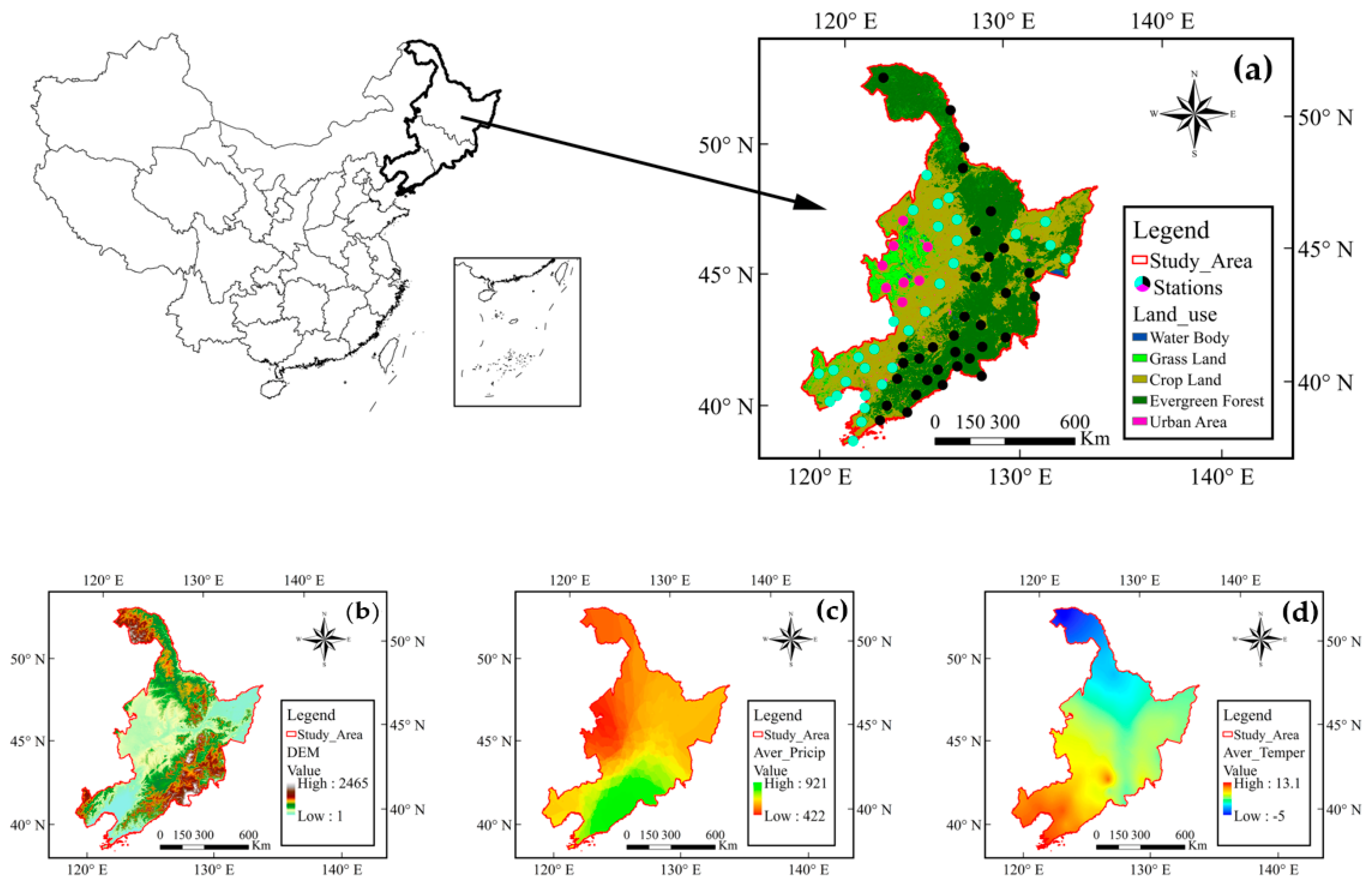
2.1. Study Area

The study (Figure 1) was conducted in the three provinces (i.e., Heilongjiang, Jilin and Liaoning) of northeastern China. These three provinces are extremely important major grain-producing areas in which total grain outputs account for a large proportion (approximately 19.3% (Statistics of 2015)) of national grain outputs [39]. The study area spans from 56°–35° N to 118.83°–135.08° E, covering an area of 7.873 × 10⁵ km2. Precipitation in the study area is dominated by the East Asian summer monsoon (EASM) [23]. Variability of EASM and related seasonal rain belts is very significant at intra-seasonal, inter-annual and inter-decadal time scales [40]. Moreover, the EASM has experienced dramatic weakening since the 1970s, and this trend is expected to aggravate drought across northeastern China [23,41].
The dominating land-cover types in the study area are cropland, sparsely vegetated grassland and evergreen or mixed forest, accounting for 45.26%, 7.42% and 45.51%, respectively, of the region as estimated from land cover classifications derived from MODIS (the Moderate Resolution Imaging Spectroradiometer) data (MCD12Q1). To quantitatively investigate how well space-borne microwave SM data monitor drought across different underlying surfaces, the study area was divided into three sub-regions corresponding to three dominant vegetation land cover types: grassland-dominated region (A), crop-dominated region (B) and evergreen forest-dominated region (C). The annual means of precipitation for the three regions amount to 411, 556 and 695 mm, respectively (as calculated using data drawn from available weather stations from 1961 to 2015). The relationship between the SMOS-SM and in situ meteorological indices of multiple scales was investigated for each of the three regions.

2.2. In Situ Reference Data and Drought Indices

Monthly precipitation and temperature data from all available stations from 1961 to 2015 were obtained from the China Meteorological Data Service Center (http://data.cma.gov.cn, accessed on 2 October 2021). Only weather stations located in the three sub-regions with complete records available from 1961 to 2015 were included. Thus, data of 8 stations in region A, 30 stations in region B and 33 stations in region C were acquired. The available water capacity (AWC) data is extracted for each weather station from the dataset by Yongjiu Dai’s research team [42] and can be found on his research group website (http://globalchange.bnu.edu.cn/research/soilw, accessed on 2 October 2021).

2.3. Remote Sensing Data

The ESA’s Soil Moisture Ocean Salinity (SMOS) Earth Explorer mission was launched in 2009. The SMOS is onboard the sun-synchronous Proteos platform, affording it global coverage with a revisit time of less than 3 days. The SMOS is equipped with a dedicated L-Band (~1.4 GHz) microwave radiometric sensor and a Microwave Imaging Radiometer with Aperture Synthesis (MIRAS) with a target accuracy of 0.04 m3/m3. L-band sensors effectively measure SM values by penetrating surfaces up to 3 to 5 cm deep depending on soil wetness levels [24,43,44]. The SMOS mission provides global SM data of approximately 0.25° in spatial resolution [45].
The satellite orbits around the earth and could not cover a certain area for every day of a month. The available soil moisture data of a month is collected by the sensor and the average value of the available data is calculated to be the monthly soil moisture. In this study, monthly SMOS-SM data provided by the SMOS website is downloaded and was compared with in situ drought indices to verify its usability in drought detecting. The closest SMOS gridded observations were searched and extracted for each in situ weather station using the nearest neighbor approach [44].

2.4. Methodologies

2.4.1. Calculation of Drought Indices

The basic theories of SPI, SPEI and sc-PDSI can be found from published articles [46,47,48]. These drought indices could be easily calculated by using the Python packages (https://pypi.org/project/climate-indices/, accessed on 2 October 2021). Ground precipitation and temperature data were aggregated by 1, 3, 6, 9 and 12 months and used to calculate in situ indices, i.e., SPIs of different time scales (SPI-1, SPI-3, SPI-6, SPI-9 and SPI-12), as well as SPEIs of different time scales (SPEI-1, SPEI-3, SPEI-6, SPEI-9 and SPEI-12). Apart from these meteorological factors, AWC is also used to calculate the sc-PDSI.
The SPI indicates how the precipitation for a specific period compares with the complete record [49]. As the main focus of this study is on agricultural drought, which depends on rainfall within 3 months, seasonal time scales of 3 to 9 months were assumed to be the most appropriate [50]. SPI-3, SPI-6 and SPI-9 values were used as reference data for measuring agricultural drought conditions. Shorter and longer time scales must also be considered, as short- and long-term droughts can seriously affect agricultural conditions. Multi-scale SPEI and PDSI values were also used as reference indices.

2.4.2. Correlation Analyses

The monthly value series of the indices from 2010 to 2015 of all the stations (or grid-based SMOS-SM near the station) for the three subset regions were obtained as previously mentioned. Pearson correlation analysis (PCA) was used to figure out whether the SMOS-SM is robust enough for detecting drought. By using PCA, the correlation coefficient could be obtained, which reflects the degree of correlation of two variables [51]. In this study, the PCA is carried out between SMOS-SM and every in situ meteorological index, i.e., 1-, 3-, 6-, 9- and 12-month SPI (SPI-1, SPI-3, SPI-6, SPI-9 and SPI-12); 1-, 3- 6-, 9- and 12-month SPEI (SPEI-1, SPEI-3, SPEI-6, SPEI-9 and SPEI-12); and sc-PDSI [22,52]. To determine whether the SMOS-SM data perform well only for the growing season or the full year, a correlation analysis was carried out for the 4-month growing season running from June to September and for each separate month. It should be noted that when the correlation analysis between two indices is carried out for a certain month, the series contain all the data of the month (e.g., there are 5 years and 8 stations for region A; there will be 40 pairs of data). If the growing season is concerned, there will be 160 pairs of data for correlation analysis. The results of these analyses were compared to investigate the performance of the SMOS-SM in monitoring drought across different forms of land cover and across seasons.

2.4.3. Spatial Comparisons between the Remotely Sensed SM and In Situ Drought Index Maps

A series of maps was generated to compare drought spatial patterns across the study area. Maps of SMOS-SM, SPI, SPEI and sc-PDSI values from 2010 to 2015 were created for July, when the yearly peak precipitation occurred over the study region. The relative soil moisture (RSM) is unusually used for the definition of drought degree; however, the field moisture capacity data is not available for RSM calculation. Exact comparisons between SMOS-SM and in situ index maps were not appropriate. Hence, the drought maps show colored dots denoting relative drought grades.

3. Results and Discussion

3.1. Relationship between SMOS-SM and In Situ Indices

Correlation coefficients were calculated between remote sensing drought SMOS-SM indices and in situ meteorological indices over three subset regions for full year and growing season (Table 1). Overall, correlation coefficients for the full year were relatively low, and most of them had a p-value > 0.05. SMOS-SM values showed relatively strong correlations with 6-, 9- and 12-month SPI and SPEI values and sc-PDSI values over the grassland region, with the p-value of these correlation coefficients passing a 0.05 confidence level test. The other correlation coefficients, except for SPI-9, were very low or negative and had a p-value of > 0.05.
For the growing season, correlation coefficients varied across regions and time scales, with most correlation coefficients exceeding 0.5. Moreover, our significance test shows that almost all of the correlation coefficients are statistically significant at the 0.01 level except for SPI-12 and SPEI-12 values for cropland and evergreen forest regions, whose p-values were found to be less than 0.05. In general, the SMOS-SM showed a relatively high correlation with all in situ meteorological indices for the growing season; thus, we focus on the growing season in the following section.
Overall, correlation coefficients over grassland were the highest followed by evergreen and cropland. Several factors may explain why lower correlations were found for cropland and evergreen forest regions. First, passive microwave-derived SM values exhibited good accordance with in situ observations over areas of low vegetation coverage to moderate density, and performance decreased as vegetation coverage increased [23,53,54]. Second, SM variations were not entirely dominated by precipitation, but were also influenced by factors such as irrigation [23]; thus, agreement between in situ indices and SMOS-SM values was relatively lower over cropland areas.
Correlations between SMOS-SM and SPI values over grassland areas first increased and then fell, for which the r values increased from 0.61 to 0.83 on SPI-9 and then decreased to 0.69. Similarly, correlations between SMOS-SM and SPEI values over grassland areas followed the same trend as SPI values, with the highest r value found between SM and SPEI-6 values. Although the sc-PDSI performed fairly well, its correlation with SMOS-SM values is not as strong as those with 3-, 6- and 9-month SPI and SPEI values.
In contrast, correlation coefficients fluctuated over cropland and evergreen forest regions, with the highest coefficients appearing in the SPI-9 (the same as those for grassland areas). The SPI-6 and SPEI-6 showed lower correlations with SMOS-SM values than 3- and 9-month SPI and SPEI values. Correlations between SMOS-SM values and 12-month SPI and SPEI values were the lowest, and their p-values did not pass a 0.01 level significance test. Correlations between SMOS-SM and PDSI values were not as strong as those for grassland areas but outperformed SPI-6 values over cropland areas. Overall, remote sensing indices showed relatively higher correlations with 3-, 6- and 9-month SPI and SPEI values and sc-PDSI values over cropland areas, according with previous findings over northern China [23]. This result suggests that the SMOS-SM product provided valuable information for monitoring agricultural droughts for the regions.

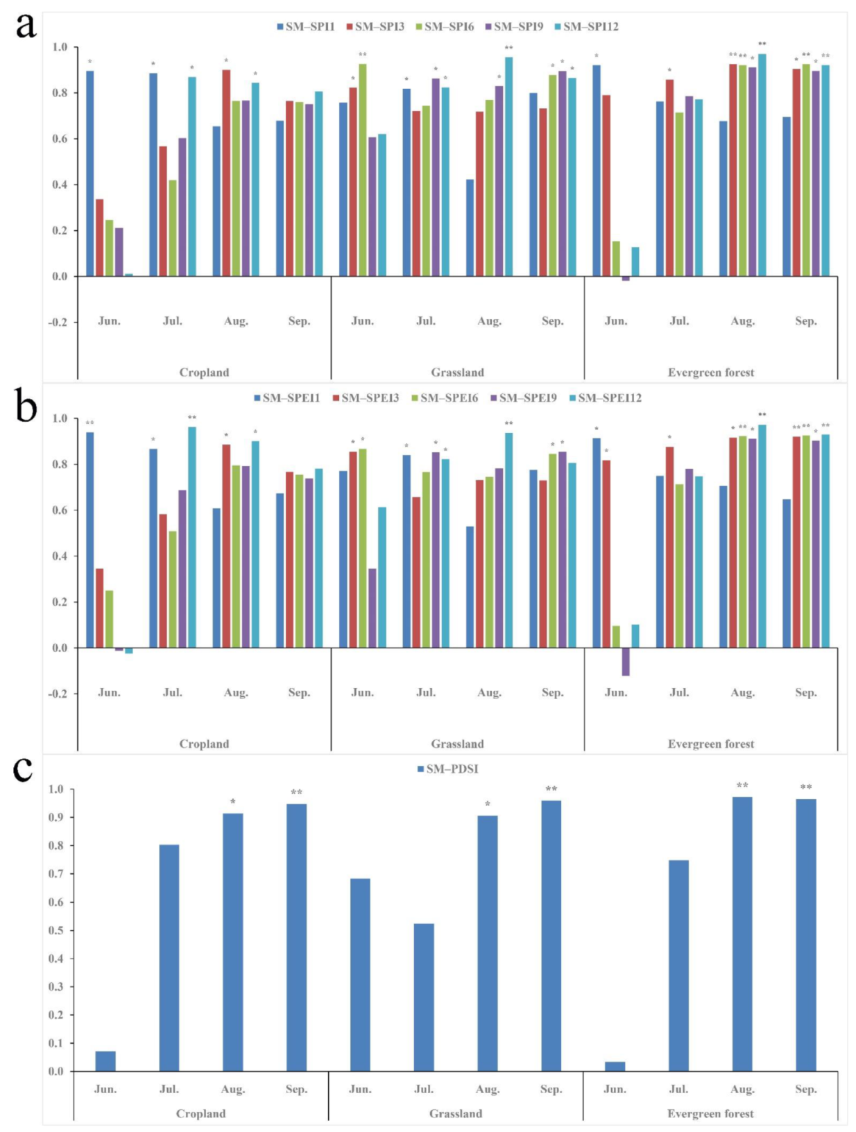
3.2. Temporal Correlation between Remote Sensing Drought Indices and In Situ Meteorological Indices

Correlation coefficients between remote sensing drought indices and in situ meteorological indices of different time scales for each month of the growing season are summarized in Figure 2. It could be noticed that the r values varied considerably over month and time scales across the regions, indicating that the SMOS-SM varies in its capacity to monitor drought conditions over seasonal time.
For the grassland-dominated region, the SMOS-SM showed strong correlations with SPIs of all time scales for each month of the growing season with the exception of the SPI-1 for August. Among them, the 3- and 6-month SPIs were closely related with the SMOS-SM in June at a high confidence level. For July, the SMOS-SM is sensitive to SPI-1. From the hot summer month of August to the end of the growing season, the long timescale SPI outperformed the short timescale SPI in correlations with the SMOS-SM. Nearly the same results were found for the correlation between the SMOS-SM and the SPEIs, although the 12-month SPEI was not closely related to the SMOS-SM for September. The sc-PDSI showed high correlations with the SMOS-SM for the last two months of the growing season. This result may be because the SMOS-SM was influenced by antecedent snowfall that melted at the beginning of the growing season, making the SMOS-SM more closely related to 3- and 6-month SPI and SPEI values. As time went on, the SM became more sensitive to temporal precipitation. At the end of the growing season, water became extremely scarce in the grassland region, so the water stored underground a long time ago may exert an influence on the SMOS-SM.
In contrast, correlations between SMOS-SM values and 1-month SPI and SPEI indices for cropland and evergreen forest areas for June showed a very distinct situation. The r values were very high, and all were statistically confident at the 0.05 or 0.01 level. Meanwhile, SPI-1 values for these two regions declined from June to September. This result may be attributed to the fact that at the beginning of the growing season vegetation coverage was not high, and its effect on remote sensing derived SMOS-SM was minor, but as vegetation grew denser, its effect became more significant. Long timescale SPIs and SPEIs and the sc-PDSI initially performed particularly poorly at the 6-, 9- and 12-month scales and gradually improved in terms of correlations with the SMOS-SM. This result indicates that the SMOS-SM is preferable when monitoring drought over moderate to long time periods, i.e., agriculture and hydrological drought.

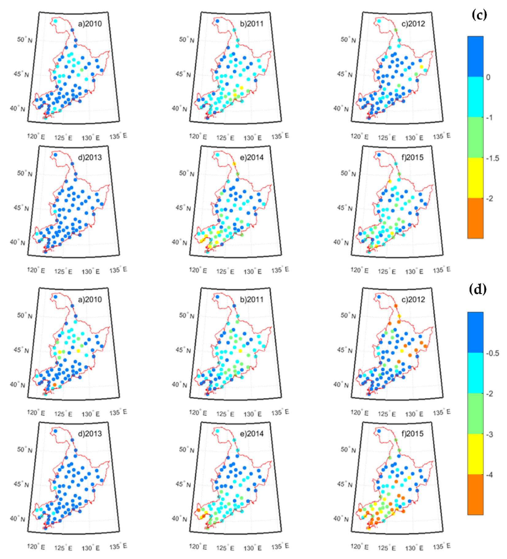
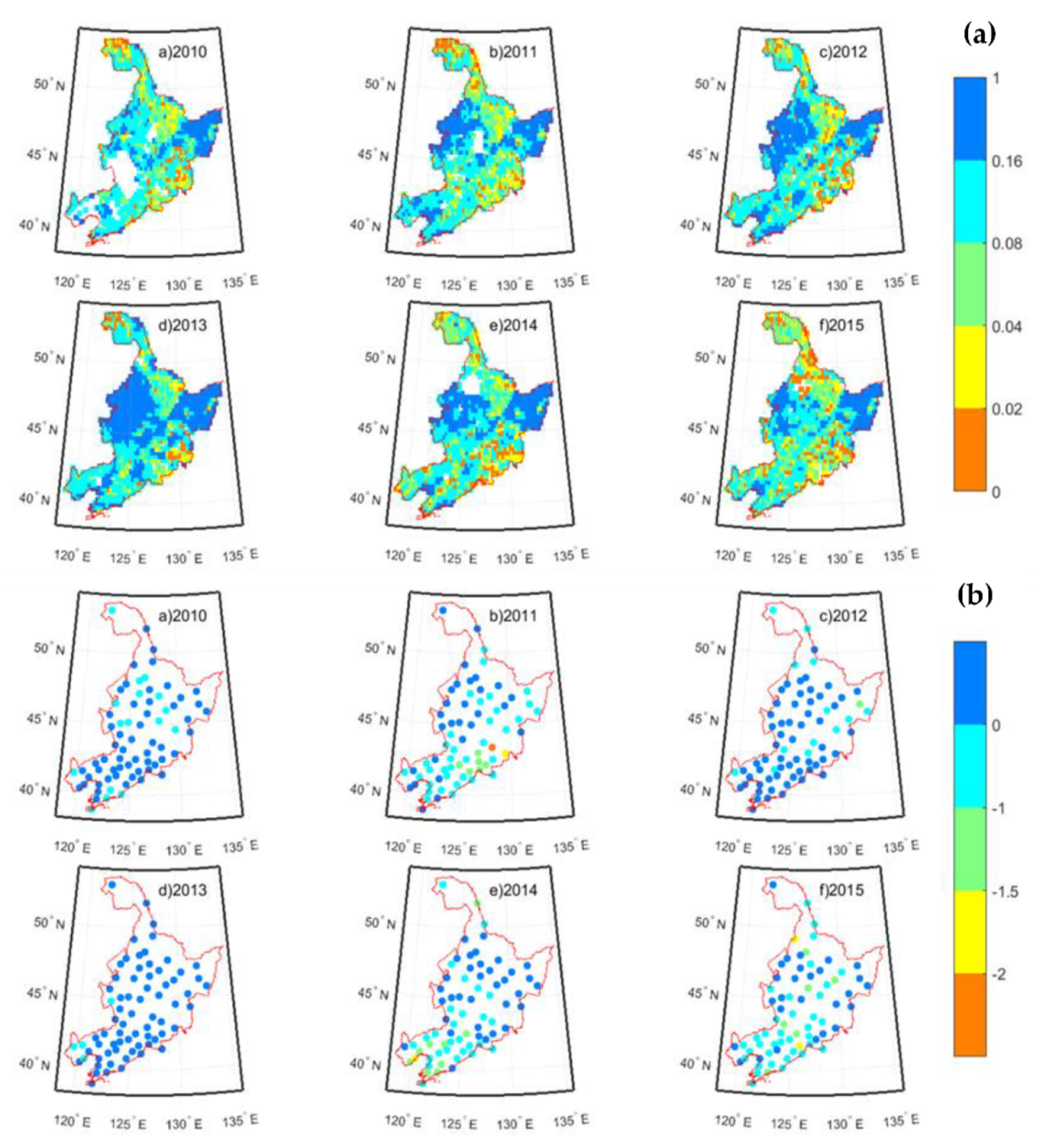
3.3. Drought Maps Based on the SMOS-SM and Comparisons to In Situ Indices

A series of drought maps was created for July of 2010–2015 based on SMOS-SM and in situ meteorological indices to compare drought spatial patterns over northeastern China (Figure 3). The in situ indices, i.e., SPIs, SPEIs and sc-PDSIs, were classified into five levels of water status, i.e., extremely dry, severely dry, moderately dry, mild dryness and normal [55,56], and are represented in orange, yellow, green, baby blue and blue (sub-figures II, III and IV of Figure 3). Since we have not obtained detailed field capacity information for each corresponding SMOS-SM grid to calculate relative water content levels, as mentioned earlier, the categories of SMOS-SM maps were classified arbitrarily for presenting purposes. Thus, the categories of SMOS-SM maps and those of in situ indices were not one-to-one relationships, although they are labeled as bars of similar colors.
In most of the study area, annual changes and spatial distributions of SMOS-SM values correspond well with the in situ indices, indicating that the remote sensing SM was successful in monitoring drought conditions in northeastern China. Drought conditions revealed through in situ indices are captured by the SM-SMOS, especially for 2011, 2014 and 2015. All three in situ index maps show that the southeastern area in 2011, the southwestern area in 2014 and the southern area in 2015 experienced moderate to severe drought while drought conditions depicted by the sc-PDSI were the most serious (sub-figure IV in Figure 3). It is evident from sub-figure I of Figure 3 that the SMOS-SM maps show few discrepancies in spatial patterns of drought conditions with in situ index maps. The most serious drought events that occurred in 2015 were reflected in the SMOS-SM and in situ maps and in the sc-PDSI maps in particular. However, the SMOS-SM maps show that in 2011, soil water levels may have been insufficient in the northwest, although this result is not reflected in in situ indices. This result may be attributed to the fact that the rainfall in this area is scarce, and soil moisture levels were low throughout the year. Thus, it is drought in the SMOM-SM map. However, the in situ indices describe water conditions in consideration of historic precipitation. Though the current rainfall may be limited, it may not be much less than the normal condition. Consequently, large-scale field moisture capacity information is indispensable when remote sensing SM is applied for drought monitoring.
Apart from serious drought conditions, the maps show relatively better water conditions, i.e., in 2010, 2012 and 2013. Water scarcity conditions during these three years were less severe. Conditions in 2013 were the most favorable, involving nearly no drought with the exception of a few moderate drought events occurring in the southeastern area. The SMOS-SM maps show better water conditions for these years compared with those of 2011, 2014 and 2015. Meanwhile, poor drought conditions in the eastern region in 2012 are reflected in the SMOS-SM and in situ maps. However, without access to detailed field capacity information, the SMOS-SM cannot compare exact categories with in situ indices. Moreover, as the SMOS-SM data only represents the soil moisture statue of the surface layer within 5 cm and may not reflect real drought condition, reinforcing the data usability by adding new information is indispensable.

4. Conclusions

In this study, passive microwave remote sensing soil moisture data, a SMOS soil moisture product, were compared to several in situ meteorological indices (SPIs, SPEIs and sc-PDSI) through a Pearson correlation analysis to validate the product’s effectiveness at monitoring agricultural drought in northeastern China. Then, drought maps of in situ indices and SMOS-SM values for July from 2010 to 2015 were generated to compare drought spatial patterns and to further test the performance of the SMOS product.
The results showed that the SMOS-SM had strong correlations with in situ indices for the growing season, but for an entire year correlation coefficients between remote sensing and in situ indices were not satisfactory. Meanwhile, the SMOS-SM showed the highest correlation with in situ indices for the grassland region, followed by evergreen areas, while for cropland areas the coefficients was the lowest correlation. Furthermore, the SMOS-SM has better correlation with the SPI-9 and SPEI-9. Hence, drought maps based on the SMOS-SM, SPI-9, SPEI-9 and sc-PDSI were created, and corresponding spatial patterns were analyzed.
The drought maps depicted by the SMOS-SM were not categorized due to a lack of large-scale field capacity information; nonetheless, they were classified artificially based on in situ indices. Overall, the SMOS-SM successfully captured drought distributions, but did not have the capacity to identify the exact drought levels. The water conditions in some areas were overestimated in relation to the in situ indices, as these meteorological indices consider historic water patterns. Overall, the SMOS product effectively monitors drought conditions in northeastern China and will perform even better as more soil survey data become available.

Author Contributions

The article was mainly written by T.C. and S.H. provided valuable advice. B.H. and J.Q. collected the data and reviewed the manuscript. B.Z. and C.T. carried out the analysis. All authors have read and agreed to the published version of the manuscript.

Funding

This research was funded by the Philosophy and Social Science planning project of Guangdong Province (Grant No. GD21YYJ15), Special Fund for Research on Public Interests, Ministry of Water Resources (Grant No. 201401036), Guangdong-Hong Kong Joint Laboratory for Water Security (Grant No. 2020B1212030005) and Guangdong Provincial Water Science and Technology Innovation Foundation (Grant No. 2017-13).

Institutional Review Board Statement

Not applicable.

Informed Consent Statement

Not applicable.

Data Availability Statement

The data presented in this study are available on request from the corresponding author. The data are not publicly available due to privacy.

Acknowledgments

The authors want to express their gratitude to China Meteorological Data Service, Yongjiu Dai’s Team and Barcelona Expert Center (BEC) for providing the basic data. The professional comments and suggestions from the anonymous reviewers are vital for the improvement of the article and we sincerely thank them.

Conflicts of Interest

There are no conflicts of interest.

References

  1. Mishra, A.K.; Singh, V.P. A review of drought concepts. J. Hydrol. 2010, 391, 202–216. [Google Scholar] [CrossRef]
  2. Tramblay, Y.; Koutroulis, A.; Samaniego, L.; Vicente-Serrano, S.M.; Volaire, F.; Boone, A.; Le Page, M.; Llasat, M.C.; Albergel, C.; Burak, S.; et al. Challenges for drought assessment in the Mediterranean region under future climate scenarios. Earth-Sci. Rev. 2020, 210, 103348. [Google Scholar]
  3. Li, J.; Wang, Z.; Wu, X.; Xu, C.Y.; Guo, S.; Chen, X.; Zhang, Z. Robust Meteorological Drought Prediction Using Antecedent SST Fluctuations and Machine Learning. Water Resour. Res. 2021, 57, e2020WR029413. [Google Scholar] [CrossRef]
  4. Li, J.; Wang, Z.; Wu, X.; Zscheischler, J.; Guo, S.; Chen, X. A standardized index for assessing sub-monthly compound dry and hot conditions with application in China. Hydrol. Earth Syst. Sci. 2021, 25, 1587–1601. [Google Scholar] [CrossRef]
  5. Zhang, J.; Xu, Y.; Yao, F.; Wang, P.; Guo, W.; Li, L.; Yang, L. Advances in estimation methods of vegetation water content based on optical remote sensing techniques. Sci. China Technol. Sci. 2010, 53, 1159–1167. [Google Scholar] [CrossRef]
  6. Zhang, J.; Zhou, Z.; Yao, F.; Yang, L.; Hao, C. Validating the modified perpendicular drought index in the north china region using in situ soil moisture measurement. IEEE Geosci. Remote Sens. Lett. 2015, 12, 542–546. [Google Scholar] [CrossRef]
  7. Vicente-Serrano, S.M.; Quiring, S.M.; Peña-Gallardo, M.; Yuan, S.; Domínguez-Castro, F. A review of environmental droughts: Increased risk under global warming? Earth-Sci. Rev. 2020, 201, 102953. [Google Scholar] [CrossRef]
  8. Wilhite, D.A.; Glantz, M.H. Understanding: The drought phenomenon: The role of definitions. Water Int. 1985, 10, 111–120. [Google Scholar] [CrossRef] [Green Version]
  9. Wu, D.; Li, Z.; Zhu, Y.; Li, X.; Wu, Y.; Fang, S. A new agricultural drought index for monitoring the water stress of winter wheat. Agric. Water Manag. 2021, 244, 106599. [Google Scholar] [CrossRef]
  10. Palmer, W. Meteorological Drought Research Paper 45; U.S. Weather Bureau: Washington, DC, USA, 1965.
  11. Gibbs, W.J.; Maher, J.V. Rainfall Deciles as Drought Indicators; Bureau of Meteorology: Melbourne, Australia, 1967.
  12. McKee, B.T.; Doesken, N.J.; Kleist, J. The relationship of drought frequency and duration to time scales. In Proceedings of the 8th Conference on Applied Climatology, Anaheim, CA, USA, 17–22 January 1993; American Meteorological Society: Boston, MA, USA, 1993. [Google Scholar]
  13. Beguería, S.; Vicente-Serrano, S.M.; Reig, F.; Latorre, B. Standardized precipitation evapotranspiration index (SPEI) revisited: Parameter fitting, evapotranspiration models, tools, datasets and drought monitoring. Int. J. Climatol. 2014, 34, 3001–3023. [Google Scholar] [CrossRef] [Green Version]
  14. Li, J.; Wang, Z.; Wu, X.; Xu, C.Y.; Guo, S.; Chen, X. Toward monitoring short-term droughts using a novel daily scale, standardized antecedent precipitation evapotranspiration index. J. Hydrometeorol. 2020, 21, 891–908. [Google Scholar] [CrossRef]
  15. Keyantash, J.; Dracup, J.A. The quantification of drought: An evaluation of drought indices. Bull. Am. Meteorol. Soc. 2002, 83, 1167. [Google Scholar] [CrossRef]
  16. Belayneh, A.; Adamowski, J.; Khalil, B.; Ozga-Zielinski, B. Long-term SPI drought forecasting in the Awash River Basin in Ethiopia using wavelet neural network and wavelet support vector regression models. J. Hydrol. 2014, 508, 418–429. [Google Scholar] [CrossRef]
  17. Kisi, O.; Gorgij, A.D.; Zounemat-Kermani, M.; Mahdavi-Meymand, A.; Kim, S. Drought forecasting using novel heuristic methods in a semi-arid environment. J. Hydrol. 2019, 578, 124053. [Google Scholar] [CrossRef]
  18. Andreadis, K.M.; Clark, E.A.; Wood, W.; Hamlet, A.F.; Lettenmaier, D.P. Twentieth-century drought in the conterminous United States. J. Hydrometeorol. 2005, 6, 985–1001. [Google Scholar] [CrossRef]
  19. Cai, W.; Cowan, T.; Briggs, P.; Raupach, M. Rising temperature depletes soil moisture and exacerbates severe drought conditions across southeast Australia. Geophys. Res. Lett. 2009, 36. [Google Scholar] [CrossRef]
  20. Carrão, H.; Sepulcre, G.; Horion, S.M.A.F.; Barbosa, P. A multitemporal and non-parametric approach for assessing the impacts of drought on vegetation greenness: A case study for Latin America. EARSeL eProceedings 2013, 12, 8–24. [Google Scholar]
  21. Vyas, S.S.; Bhattacharya, B.K.; Nigam, R.; Guhathakurta, P.; Ghosh, K.; Chattopadhyay, N.; Gairola, R.M. A combined deficit index for regional agricultural drought assessment over semi-arid tract of India using geostationary meteorological satellite data. Int. J. Appl. Earth Obs. Geoinf. 2015, 39, 28–39. [Google Scholar] [CrossRef]
  22. Rhee, J.; Im, J.; Carbone, G.J. Monitoring agricultural drought for arid and humid regions using multi-sensor remote sensing data. Remote Sens. Environ. 2010, 114, 2875–2887. [Google Scholar] [CrossRef]
  23. Zhang, A.; Jia, G. Monitoring meteorological drought in semiarid regions using multi-sensor microwave remote sensing data. Remote Sens. Environ. 2013, 134, 12–23. [Google Scholar] [CrossRef]
  24. Sánchez, N.; González-Zamora, Á.; Piles, M.; Martínez-Fernández, J. A New Soil Moisture Agricultural Drought Index (SMADI) Integrating MODIS and SMOS Products: A Case of Study over the Iberian Peninsula. Remote Sens. 2016, 8, 287. [Google Scholar] [CrossRef] [Green Version]
  25. West, H.; Quinn, N.; Horswell, M. Remote sensing for drought monitoring & impact assessment: Progress, past challenges and future opportunities. Remote Sens. Environ. 2019, 232, 111291. [Google Scholar]
  26. Liu, Q.; Zhang, S.; Zhang, H.; Bai, Y.; Zhang, J. Monitoring drought using composite drought indices based on remote sensing. Sci. Total Environ. 2020, 711, 134585. [Google Scholar] [CrossRef] [PubMed]
  27. Avtar, R.; Komolafe, A.A.; Kouser, A.; Singh, D.; Yunus, A.P.; Dou, J.; Kumar, P.; Gupta, R.D.; Johnson, B.A.; Minh, H.V.T.; et al. Assessing sustainable development prospects through remote sensing: A review. Remote Sens. Appl. Soc. Environ. 2020, 20, 100402. [Google Scholar] [CrossRef]
  28. Liu, Y.Y.; Parinussa, R.; Dorigo, W.A.; de Jeu, R.A.; Wagner, W.; van Dijk, A.; McCabe, M.F.; Evans, J. Developing an improved soil moisture dataset by blending passive and active microwave satellite-based retrievals. Hydrol. Earth Syst. Sci. 2011, 15, 425–436. [Google Scholar] [CrossRef] [Green Version]
  29. Ford, T.; Harris, E.; Quiring, S. Estimating root zone soil moisture using near-surface observations from SMOS. Hydrol. Earth Syst. Sci. 2014, 18, 139–154. [Google Scholar] [CrossRef] [Green Version]
  30. Kim, S.; Liu, Y.Y.; Johnson, F.M.; Parinussa, R.M.; Sharma, A. A global comparison of alternate AMSR2 soil moisture products: Why do they differ? Remote Sens. Environ. 2015, 161, 43–62. [Google Scholar] [CrossRef]
  31. Colliander, A.; Njoku, E.G.; Jackson, T.J.; Chazanoff, S.; McNairn, H.; Powers, J.; Cosh, M.H. Retrieving soil moisture for non-forested areas using PALS radiometer measurements in SMAPVEX12 field campaign. Remote Sens. Environ. 2016, 184, 86–100. [Google Scholar] [CrossRef]
  32. Vergopolan, N.; Chaney, N.W.; Beck, H.E.; Pan, M.; Sheffield, J.; Chan, S.; Wood, E.F. Combining hyper-resolution land surface modeling with SMAP brightness temperatures to obtain 30-m soil moisture estimates. Remote Sens. Environ. 2020, 242, 111740. [Google Scholar] [CrossRef]
  33. Leroux, D.J.; Kerr, Y.H.; al Bitar, A.; Bindlish, R.; Jackson, T.J.; Berthelot, B.; Portet, G. Comparison between SMOS, VUA, ASCAT, and ECMWF soil moisture products over four watersheds in US. IEEE Trans. Geosci. Remote Sens. 2014, 52, 1562–1571. [Google Scholar] [CrossRef] [Green Version]
  34. Kerr, Y.H.; Waldteufel, P.; Wigneron, J.-P.; Delwart, S.; Cabot, F.; Boutin, J.; Escorihuela, M.-J.; Font, J.; Reul, N.; Gruhier, C. The SMOS mission: New tool for monitoring key elements ofthe global water cycle. Proc. IEEE 2010, 98, 666–687. [Google Scholar] [CrossRef] [Green Version]
  35. Entekhabi, D.; Yueh, S.; O’Neill, P.; Kellogg, K.; Allen, A.; Bindlish, R.; Brown, M.; Chan, S.; Colliander, A.; Crow, W.T.; et al. SMAP Handbook-Soil Moisture Active Passive: Mapping Soil Moisture and Freeze/Thaw from Space; JPL Publication: Pasadena, CA, USA, 2014; pp. 400–1567.
  36. Du, L.; Tian, Q.; Yu, T.; Meng, Q.; Jancso, T.; Udvardy, P.; Huang, Y. A comprehensive drought monitoring method integrating MODIS and TRMM data. Int. J. Appl. Earth Obs. Geoinf. 2013, 23, 245–253. [Google Scholar] [CrossRef]
  37. Arun Kumar, K.C.; Reddy, G.P.O.; Masilamani, P.; Turkar, S.Y.; Sandeep, P. Integrated drought monitoring index: A tool to monitor agricultural drought by using time-series datasets of space-based earth observation satellites. Adv. Space Res. 2021, 67, 298–315. [Google Scholar] [CrossRef]
  38. Sandeep, P.; Reddy, G.P.O.; Jegankumar, R.; Kumar, K.C.A. Monitoring of agricultural drought in semi-arid ecosystem of Peninsular India through indices derived from time-series CHIRPS and MODIS datasets. Ecol. Indic. 2021, 121, 107033. [Google Scholar] [CrossRef]
  39. National Bureau of Statistics of China. China Statistical Yearbook; China Statistics Press: Beijing, China, 2015.
  40. Ding, Y. The variability of the asian summer monsoon. J. Meteorol. Soc. Jpn. 2007, 85, 21–54. [Google Scholar] [CrossRef] [Green Version]
  41. Ding, Y.; Wang, Z.; Sun, Y. Inter-decadal variation of the summer precipitation in East China and its association with decreasing Asian summer monsoon. Part I: Observed evidences. Int. J. Climatol. 2008, 28, 1139–1161. [Google Scholar] [CrossRef]
  42. Shangguan, W.; Dai, Y.; Duan, Q.; Liu, B.; Yuan, H. A Global Soil Data Set for Earth System Modeling. J. Adv. Modeling Earth Syst. 2014, 6, 249–263. [Google Scholar] [CrossRef]
  43. Chakravorty, A.; Chahar, B.R.; Sharma, O.P.; Dhanya, C.T. A regional scale performance evaluation of SMOS and ESA-CCI soil moisture products over India with simulated soil moisture from MERRA-Land. Remote Sens. Environ. 2016, 186, 514–527. [Google Scholar] [CrossRef]
  44. Fascetti, F.; Pierdicca, N.; Pulvirenti, L.; Crapolicchio, R.; Muñoz-Sabater, J. A comparison of ASCAT and SMOS soil moisture retrievals over Europe and northern Africa from 2010 to 2013. Int. J. Appl. Earth Obs. Geoinf. 2016, 45, 135–142. [Google Scholar] [CrossRef]
  45. Louvet, S.; Pellarin, T.; al Bitar, A.; Cappelaere, B.; Galle, S.; Grippa, M.; Gruhier, C.; Kerr, Y.; Lebel, T.; Mialon, A. SMOS soil moisture product evaluation over West-Africa from local to regional scale. Remote Sens. Environ. 2015, 156, 383–394. [Google Scholar] [CrossRef]
  46. Asadi Zarch, M.A.; Sivakumar, B.; Sharma, A. Droughts in a warming climate: A global assessment of Standardized precipitation index (SPI) and Reconnaissance drought index (RDI). J. Hydrol. 2015, 526, 183–195. [Google Scholar] [CrossRef]
  47. Banimahd, S.A.; Khalili, D. Factors influencing markov chains predictability characteristics, utilizing spi, rdi, edi and spei drought indices in different climatic zones. Water Resour. Manag. 2013, 27, 3911–3928. [Google Scholar] [CrossRef]
  48. Wells, N.; Goddard, S.; Hayes, M.J. A self-calibrating palmer drought severity index. J. Clim. 2004, 17, 2335–2351. [Google Scholar] [CrossRef]
  49. Patel, N.R.; Chopra, P.; Dadhwal, V.K. Analyzing spatial patterns of meteorological drought using standardized precipitation index. Meteorol. Appl. 2007, 14, 329–336. [Google Scholar] [CrossRef]
  50. Rouault, M.; Richard, Y. Intensity and spatial extension of droughts in South Africa at different time scales. Water SA 2003, 29, 489–500. [Google Scholar] [CrossRef] [Green Version]
  51. Ding, Y.B.; Gong, X.L.; Xing, Z.X. Attribution of meteorological, hydrological and agricultural drought propagation in different climatic regions of China. Agric. Water Manag. 2021, 255, 106996. [Google Scholar] [CrossRef]
  52. Guttman, N.B. Accepting the standardized precipitation index: A calculation algorithm. J. Am. Water Resour. Assoc. 1999, 35, 311–322. [Google Scholar] [CrossRef]
  53. Owe, M.; de Jeu, R.; Holmes, T. Multisensor historical climatology of satellite-derived global land surface moisture. J. Geophys. Res. Earth Surf. 2008, 113. [Google Scholar] [CrossRef]
  54. Liu, Y.; Dorigo, W.A.; Parinussa, R.; de Jeu, R.A.; Wagner, W.; McCabe, M.F.; Evans, J.; van Dijk, A. Trend-preserving blending of passive and active microwave soil moisture retrievals. Remote Sens. Environ. 2012, 123, 280–297. [Google Scholar] [CrossRef]
  55. Schrier, G.V.D.; Barichivich, J.; Briffa, K.R.; Jones, P.D. A scPDSI-based global data set of dry and wet spells for 1901–2009. J. Geophys. Res. 2013, 118, 4025–4048. [Google Scholar] [CrossRef]
  56. Xu, K.; Yang, D.; Yang, H.; Li, Z.; Qin, Y.; Shen, Y. Spatio-temporal variation of drought in China during 1961–2012: A climatic perspective. J. Hydrol. 2015, 526, 253–264. [Google Scholar] [CrossRef]
Figure 1. Study area and climate characteristics. (a) Vegetation regionalization from MODIS MCD12Q1 land cover type data and meteorological station distribution according to the China Meteorological Data Service Center; (b) DEM data downloaded from the Geospatial Data Cloud website (i.e., http://www.gscloud.cn/, accessed on 2 October 2021); (c,d) average annual precipitation and temperature distributions for 1961 to 2015 according to 71 meteorological stations across northeastern China.
Water 13 02777 g001
Figure 2. Correlations between SMOS-SM and in situ indices of different time scales across three sub-regions for each month of the growing season from June to September. The three sub-graphs from top to bottom show the correlation coefficients between the SMOS-SM and in situ indices (sub-figure (a) for SPIs, sub-figure; (b) for SPEIs and sub-figure; (c) for PDSI). p-value < 0.01 for columns with double asterisk (**) and p-value < 0.05 for columns with single asterisk (*).
Water 13 02777 g002
Figure 3. Annual maps of SMOS-SM and in situ meteorological indices for July of 2010 to 2015. Sub-figures (ad) refer to SMOS-SM, SPI-9, SPEI-9 and PDSI data, respectively.
Water 13 02777 g003aWater 13 02777 g003b
Table 1. Correlations between SMOS-SM and in situ indices of different time scales for the three sub-regions for full year and growing season, respectively. For the “Full Year” column, r values with p-value < 0.05 are underlined and italicized. For the “Growing Season” column, the highest r values for each row for the three regions are shown in italics/bold. The p-value < 0.01 except for data with asterisk (*), for which the p-value < 0.05.
In Situ IndicesFull YearGrowing Season
CroplandGrasslandEvergreen ForestCroplandGrasslandEvergreen Forest
SPI-10.040.060.10.60.610.59
SPI-3−0.040.1−0.030.650.780.66
SPI-60.150.390.130.530.820.59
SPI-90.240.480.180.660.830.66
SPI-120.110.250.110.43 *0.690.46 *
SPEI-1−0.03000.560.630.54
SPEI-3−0.080.06−0.090.610.770.64
SPEI-60.090.350.060.530.810.59
SPEI-90.180.450.150.630.780.66
SPEI-120.090.260.110.47 *0.690.47 *
sc-PDSI0.050.320.060.580.760.53
Publisher’s Note: MDPI stays neutral with regard to jurisdictional claims in published maps and institutional affiliations.

