Impacts of Climate Change on Urban Drainage Systems by Future Short-Duration Design Rainstorms

Abstract

The adverse impacts of climate change and urbanization are converging to challenge the waterlogging control measures established in the Dong Hao Chong (DHC) Basin. Based on representative concentration pathway (RCP) scenarios, the future (2030–2050) waterlogging was assessed for the DHC basin and combined with future design rainfall. The delta change factors were projected using the regional climate model, RegCM4.6, and the annual maximum one-day rainstorm was modified to develop the annual maximum value method. By combining the delta change and annual maximum value methods, a future short-duration design rainstorm formula is developed in this study. The Chicago hyetograph shapes indicated that the peak rainfall intensity and amount both increase in the five return periods with two RCP scenarios. The InfoWorks ICM urban flood model is used to simulate the hydrological response. The results show that climate change will exacerbate urban waterlogging in DHC Basin. The maximum inundation volume and number of inundation nodes were expected to increase in the five return periods under the RCP4.5 and RCP8.5 scenarios, respectively. The submerged area is increasing due to climate change. This study highlights the link between climate change and urban drainage systems, and suggests that the effect of climate change in extreme rainfall should be considered in urban waterlogging management and drainage system design.

1. Introduction

The atmospheric concentrations of greenhouse gases have been increasing since industrialization due to human activity, and have led to significant climate change that intensifies the global hydrological cycle and influences climatology characteristics. Rainfall will become more uneven and intense [1], and such variations in rainfall have had serious impacts on urban flooding in recent years [2].

General circulation models (GCMs) are a class of computer-driven models for understanding the historical climate and projecting future climate change, and are considered to be the most reliable resources that are currently available for investigating and predicting climate change [3,4,5]. However, the resolution of GCM outputs tends to be coarse and cannot be used directly in hydrological modeling for regional climate impact studies. A regional climate model (RCM) can ameliorate this deficiency and its high resolution can capture smaller-scale topography and land surface characteristics better, providing more detailed information regarding local climate change as compared to GCMs [6,7]. Consequently, RCMs have been used extensively to assess regional climate change and extremes. Gao et al. [8] projected changes in extreme precipitation using the RegCM3 over the Mediterranean region, and their results suggested that the distribution of precipitation shifted and broadened, with an increased probability of events that might result in flooding. Ji et al. [9] conducted a RegCM4 downscaling projection over China, as RegCM can provide more reliable future climate change predictions at regional to local scales. Climate change has affected urban floods in recent years, and has also increased the uncertainties in flood management [10].

Several catastrophic rainstorm events have occurred in the past few years [11,12]. Consequently, inundation control and urban drainage systems will encounter substantial challenges [13,14]. Many cities have recently faced extreme rainfall events, which have resulted in enormous economic losses, injuries, and mortalities [15]. For instance, in England, the rain depth for the period of May to July 2007 was 406 mm, but a new 24 h rainfall record (316 mm) was observed at Seathwaite, Borrowdale, in 2009 [16]. An extreme rainfall event hit Beijing on 22 July 2012, with a record rainfall amount of 460 mm, which inundated many roads with trapped cars and buses, as well as collapsed buildings, in waist-deep water [17]. Many researchers state that the pressure on the urban drainage system is expected to increase [18,19]. Improved inundation risk management in response to the increased inundation risk is important [20].

Urban drainage systems are important infrastructural components in urban areas due to the high potential of flooding in these regions [21,22]. The operation of drainage systems is an issue of great importance as they affect daily urban activities [23]. The design and operation of an urban drainage system are closely associated with the rainfall characteristics of the local urban area, especially the intensity and amount of rainfall. The increasing global mean temperature has been of concern for several years as increasing temperatures intensify the hydrological cycle accordingly, and a larger number of heavy precipitation events will likely occur in the 21st century, according to the Intergovernmental Panel on Climate Change [24]. When assessing the impact of climate change, especially precipitation changes, on a city through the urban drainage system, some problems need to be considered. Two of the main problems are: (1) the type of input rainfall data used for model simulations to represent future change, and (2) how the urban drainage impacts should be measured to reflect and accurately describe the event and system characteristics [25]. A direct approach for using climate model information and change factors is the ′′delta change method′′ [26,27]. Semadeni-Davies et al. [19] used the delta change approach for urban hydrology, and compared present and future climate simulations from a regional climate model to determine monthly changes that were then applied to observed rainfall data in two groups (drizzle and storm). Olsson et al. [28] further developed this approach with more focus on rainfall intensity, and used a regional climate model to compare a control period (present time) and future periods. These generated factors considered rainfall with different intensities and differences according to the time of year (summer, autumn, winter, and spring).

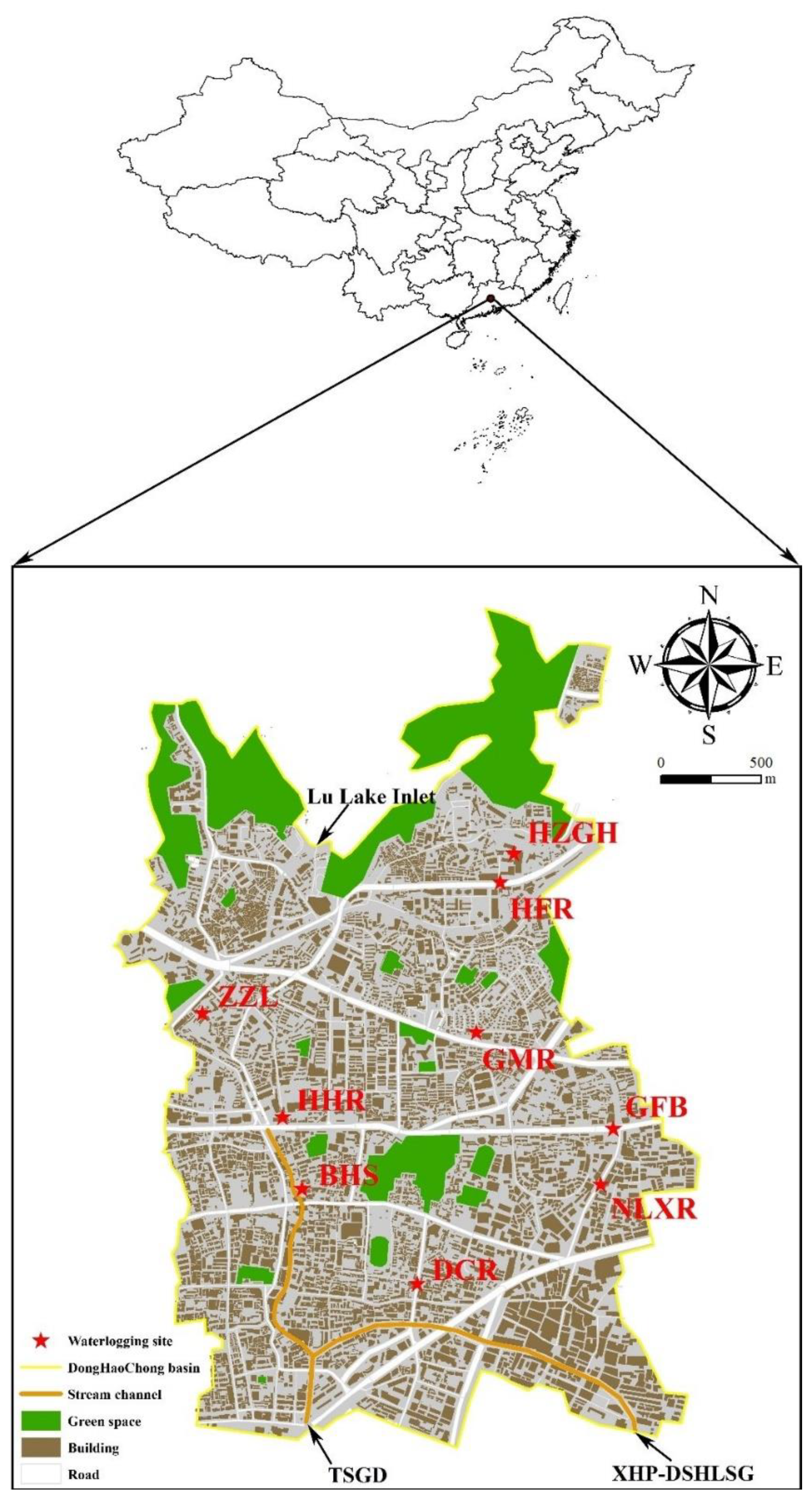
Previous studies usually relied on observed rainfall, with less consideration of design rainfall. In this study, an algorithm based on the delta change and annual maximum value methods was developed to derive future short-duration design rainfall. This algorithm evaluates the effects of climate change on the urban flood regime and characteristics. To achieve these objectives, the following three steps are followed: (1) the rainstorm intensity formula is derived considering climate change in this study. (2) The impact of climate change on urban inundation is considered. (3) The impact of climate change on urban waterlogging is considered. This paper is organized as follows: the study area is introduced in the following section; subsequently, the model and methodologies are presented. This is followed by a section which presents the results and discussions; finally the main findings are summarized in the conclusion. The findings can be further utilized in the development of appropriate urban runoff management schemes and drainage system designs for the local climate.

2. Study Area and Data

The study area is Dong Hao Chong (DHC) Basin, located in the Yuexiu District of Guangzhou, South China (Figure 1). The basin is approximately 12.403 km², and DHC River crosses the basin. The river is approximately 4.37 km long, originating from Lu Lake in the north and ending at the Pearl River in the south. It has been divided into northern and southern sections by the sewage interception sluice gate of DHC basin. The Xinhepu-Dongshan Lake sluice gate (XHP-DSHLSG) and tidal sluice gate of DHC basin (TSGD) have also been constructed in the DHC Basin [29].

3. Methodology

3.1. Delta Change Method

Delta change is commonly used to transfer the signal of climate models to hydrological models by manipulating the observed input data. The method compares present and future climate simulations generated by the climate model to determine monthly change anomalies, which are then applied to observed data from current or historical records. Therefore, for precipitation, the delta change anomaly is the percentage increase or decrease in the average monthly or seasonal precipitation, and observations are scaled up or down accordingly. There are two main assumptions: (a) the progressive GCM runs simulate the relative changes in climate, rather than absolute changes; and (b) there is no change in the number of precipitation events (i.e., rain-days) [19,26]. In this study, the monthly and ordinary daily change factors are abandoned and substituted with the annual maximum daily rainfall change factor to correspond with the method for deriving the urban storm intensity.

The major advantage of delta-change is its simplicity, i.e., the climate model output data require no manipulation. As an existing data set forms the basis of the transformation, the impact of climate change on individual storms and the response of the hydrological system to those storms can be compared. In the case of the DHC Basin, both the RCP4.5 (representative concentration pathway) and RCP8.5 scenarios predict increasing annual maximum one-day rainfall. Once the delta change factors were determined, the change in rainfall is tagged and adjusted accordingly.

3.2. Deriving the Future Urban Rainstorm Intensity Formula

3.2.1. Annual Maximum Value Method

The annual maximum value method (AMVM) is selected to represent the annual maximum rainfall for each timescale [30]. The extreme value theory indicates that long rainfall series data can be taken as all data series. The AMVM requires a rainfall data series of at least 20a. The experience frequency (P_M) and return period (T_M) are represented in the AMVM as follows:

$$P_M=\frac{m}{N+1}$$

(1)

$$T_M=\frac{N+1}{m}$$

(2)

where m indicates the sequence of rainfall data in decreasing order, and N represents the number of rainfall data years.

In this study, 30a of observed short-duration rainfall data (1984–2013) at 5, 10, 15, 20, 30, 45, 60, 90, and 120 min timescales were applied to generate the design rainfall formula. Only one maximum rainfall was selected for each timescale. The rainfall data were then ordered regardless of time series, and the intensity of 30 rainfall samples was calculated for each timescale. The delta factor was multiplied by each time-scale rainfall data to represent a future short-duration rainfall series under two RCP scenarios.

3.2.2. Design Short-Duration Frequency Analysis

Extreme rainfall is a random event, and there is still no consensus regarding extreme rainfall curve fitting. In this study, we use the Pearson Type 3 (P-3) distribution to analyze the extreme rainfall frequency, which is widely used in hydrology [31,32]. The theoretical frequency curve analysis is conducted based on the P-3 distribution to obtain the intensity–duration–frequency curve relationship table and calculate the storm intensity formula.

3.2.3. Urban Design Rainstorm-Intensity Formulas and Rainstorm Profile

The Technical Guidelines for the Establishment of an Intensity–Duration–Frequency Curve and Design Rainstorm Profile recommend using formula (1) to compile urban design rainstorm intensity formulae [33].

$$q=\frac{167A_1(1+C\lg P)}{{(t+b)}^n}$$

(3)

where q represents the rainstorm intensity (mm/min), t represents the rainstorm duration (min), A represents the 1-min amount of rainstorms when the rainstorm return period is 1a, C is the rainstorm parameter, b is the modified rainstorm-duration parameter, and n is the rainstorm-decay parameter. The Chicago hyetograph method is used to identify the rainstorm profile [34]. The peak intensity position coefficient is set at 0.415 with a 5 min interval.

3.2.4. Climate Model

The regional climate model version 4.6 (RegCM4.6), developed by the Abdus Salam International Center for Theoretical Physics (ICTP), is a hydrostatic equilibrium model with a dynamic core based on the mesoscale model MM5 from NCAR/PSU [35]. The radiative transfer package is included in the NCAR Community Climate Model 3.0 (CCM3) [36], and the Biosphere-Atmosphere Transfer Scheme is used as the land surface module (BATS1e) [37]. The non-local boundary scheme was obtained from Holtslag et al. [38], and the ocean flux parameterization follows Zeng et al. [39]. The experiments in this study were configured using the mass flux convective precipitation scheme from Grell [35] and the Arakawa and Schubert-type closure assumption [40].

The initial and lateral boundary conditions were obtained from the Geophysical Fluid Dynamics Laboratory Earth System Model version 2M, with a horizontal resolution of 2.5 × 2.0° (GFDL-ESM-2M) [41,42]. Since GFDL-ESM-2 M is independent and has a good performance in recent climate simulation for the Zhujiang River Basin, it can be used for the initial and lateral boundary conditions in this study. The boundary conditions were updated four times per day. The sea surface temperature (SST) was retrieved from the GCM outputs. The land use and satellite data obtained by the United States Geological Survey (USGS) were provided by the Global Land Cover Characterization (GLCC) [43]. The horizontal resolution of the model was set to 20 km. There are 18 vertical layers arranged on sigma levels, with the model top at 10 hPa. The simulation period was divided into two sub-periods: the reference (RF) 1979–2000 and future periods 2029–2050 under the RCP4.5 and RCP8.5 scenarios. The first year of each simulation was regarded as a spin-up period, and will not be considered in further analyses. The timestep is set up in 45s.

3.2.5. Urban Flood Model

InfoWorks Integrated Catchment Management (InfoWorks ICM 7.0) is the first truly integrated modeling platform to incorporate both urban and river catchments. With the full integration of 1-D and 2-D hydrodynamic simulation techniques, both the above- and below-ground elements of catchments can be modeled to accurately represent all flow paths. InfoWorks ICM allows the hydraulics and hydrology of natural and anthropogenic environments to be incorporated into a single model. The model mainly includes rainfall runoff, pipe network flow, channel hydraulic, two-dimensional urban flooding, real-time control, and structure modules. In the hydraulic calculation of pipes and canals, the pipe and open channel flows are simulated by solving the complete Saint Venant equations, and the overloaded pipe flow is simulated following the Preissmann slot method, which can simulate a variety of complicated hydraulic conditions. This model is used in the design, analysis, and planning of drainage systems, and for simulating runoff quality and quantity in urban areas [44,45,46]. Therefore, Info Works ICM is considered to be one of the best hydrological models.

4. Results

4.1. Future Climate Change

The performance of RCM downscaling outputs is evaluated by comparing with the observations of 15 meteorological stations, on the basis of the mean error (ME), root mean squared error (RMSE), temporal correlation coefficient (TCC) and spatial correlation coefficient (SCC). The RCM can reasonably capture the intra-annual variability of precipitation (figure not displayed), although there are still some biases between the simulations and observations. The annual ME, RMSE, TCC, and SCC is −29.03%, 33.73 mm, 0.95, and 0.53, respectively.

The simulations of CDD, Rx1day, R25mm, and Rx5day is compared with the observations (figure not displayed). For CDD, the simulations results have a well performance with the observations, with an average overestimation of 2.77%. The Rx1day, Rx5day and R25mm tend to be underestimated by 33%, 24%, and 12.74 days, respectively, which indicates an uncertainty involved in RCM for reproducing extreme precipitation events. However, overall, the RCM can reproduce precipitation extremes and is therefore judged to be applicable for the study area.

4.2. Future Design Short Duration Rainstorm Pattern

Table 1. The parameters of Pearson-3 type distribution for reference (RF) period.

Parameters	Rainfall Duration
	5 min	10 min	15 min	20 min	30 min	45 min	60 min	90 min	120 min
$\overline{x}$	2.780	2.350	2.060	1.830	1.510	1.190	0.993	0.735	0.603
Cv	0.174	0.179	0.193	0.225	0.272	0.298	0.313	0.339	0.376
Cs	0.811	0.696	0.633	0.425	0.650	0.584	0.457	0.766	1.418

,

Table 2. Same as Table 1 but for representative concentration pathway (RCP) 4.5 scenario.

Parameters	Rainfall Duration
	5 min	10 min	15 min	20 min	30 min	45 min	60 min	90 min	120 min
$\overline{x}$	2.880	2.440	2.130	1.900	1.560	1.230	1.030	0.760	0.620
Cv	0.174	0.200	0.220	0.240	0.272	0.298	0.315	0.340	0.375
Cs	0.802	0.920	0.800	0.451	0.634	0.587	0.450	0.779	1.395

and

Table 3. Same as Table 1 but for RCP8.5 scenario.

Parameters	Rainstorm Duration
	5 min	10 min	15 min	20 min	30 min	45 min	60min	90 min	120 min
$\overline{x}$	3.680	3.110	2.720	2.420	1.990	1.570	1.310	0.971	0.796
Cv	0.190	0.200	0.210	0.225	0.272	0.297	0.314	0.341	0.376
Cs	0.950	0.880	0.771	0.434	0.642	0.585	0.452	0.757	1.402

represent the Pearson-3 curve fitting, and

Table 4. The relation of intensity–duration–frequency for RF period (units: mm/min).

Rainstorm Return Period	Rainstorm Duration
	5 min	10 min	15 min	20 min	30 min	45 min	60 min	90 min	120 min
2a	2.720	2.300	2.020	1.800	1.470	1.160	0.969	0.703	0.551
3a	2.930	2.490	2.190	1.980	1.650	1.310	1.110	0.814	0.649
5a	3.160	2.680	2.380	2.170	1.840	1.470	1.250	0.930	0.762
10a	3.430	2.910	2.590	2.370	2.060	1.660	1.400	1.070	0.906
20a	3.670	3.110	2.780	2.550	2.250	1.830	1.540	1.190	1.040
30a	3.810	3.230	2.880	2.650	2.360	1.920	1.620	1.260	1.120

,

Table 5. Same as Table 4 but for RCP4.5 scenario (units: mm/min).

Rainstorm Return Period	Rainstorm Duration
	5 min	10 min	15 min	20 min	30 min	45 min	60 min	90 min	120 min
2a	2.810	2.390	2.090	1.870	1.520	1.190	1.010	0.728	0.570
3a	3.040	2.580	2.270	2.070	1.700	1.360	1.150	0.842	0.672
5a	3.270	2.790	2.460	2.270	1.900	1.520	1.290	0.963	0.788
10a	3.550	3.020	2.680	2.500	2.120	1.720	1.460	1.110	0.935
20a	3.800	3.230	2.870	2.700	2.330	1.890	1.600	1.240	1.080
30a	3.940	3.350	2.980	2.810	2.440	1.980	1.680	1.310	1.160

and

Table 6. Same as Table 4 but for RCP8.5 scenario (units: mm/min).

Rainstorm Return Period	Rainstorm Duration
	5 min	10 min	15 min	20 min	30 min	45 min	60 min	90 min	120 min
2a	3.570	3.020	2.650	2.380	1.930	1.520	1.280	0.930	0.728
3a	3.880	3.290	2.900	2.620	2.170	1.730	1.460	1.080	0.858
5a	4.210	3.590	3.170	2.860	2.420	1.940	1.640	1.230	1.010
10a	4.620	3.940	3.480	3.140	2.710	2.190	1.850	1.410	1.200
20a	4.990	4.260	3.770	3.380	2.970	2.410	2.040	1.580	1.380
30a	5.190	4.440	3.910	3.510	3.110	2.520	2.130	1.670	1.480

show the relationship between the intensity, duration, and frequency of rainstorms under the control period, RCP4.5, and RCP8.5, respectively.

Table 7. The parameter of rainstorm intensity formula.

Scenarios	A	C	b	n	${\mathit{\sigma }}_1$	${\mathit{\sigma }}_2$
Control Period	27.726	0.443	19.721	0.771	0.060	3.35%
RCP4.5	31.653	0.447	20.914	0.790	0.065	3.55%
RCP8.5	33.283	0.484	18.059	0.759	0.069	2.77%

${\sigma }_1$: Root mean square error; ${\sigma }_2$: Relative root mean square error.

shows the parameters of the urban design rainstorm intensity. The results indicate that the rRMSE of the reference period, RCP4.5, and RCP8.5 did not exceed 5%, and the RMSE values are 0.06, 0.065, and 0.069 mm/min, respectively [33]. Finally, the design rainstorm formula under climate change can be represented as follows:

$$\mathrm{Reference} \mathrm{period} q=\frac{4630.242\times (1+0.443\times \lg P)}{{(t+19.721)}^{0.771}}$$

(4)

$$\mathrm{RCP}4.5 q=\frac{5286.051\times (1+0.447\times \lg P)}{{(t+20.914)}^{0.790}}$$

(5)

$$\mathrm{RCP}8.5 q=\frac{5558.261\times (1+0.484\times \lg P)}{{(t+18.059)}^{0.759}}$$

(6)

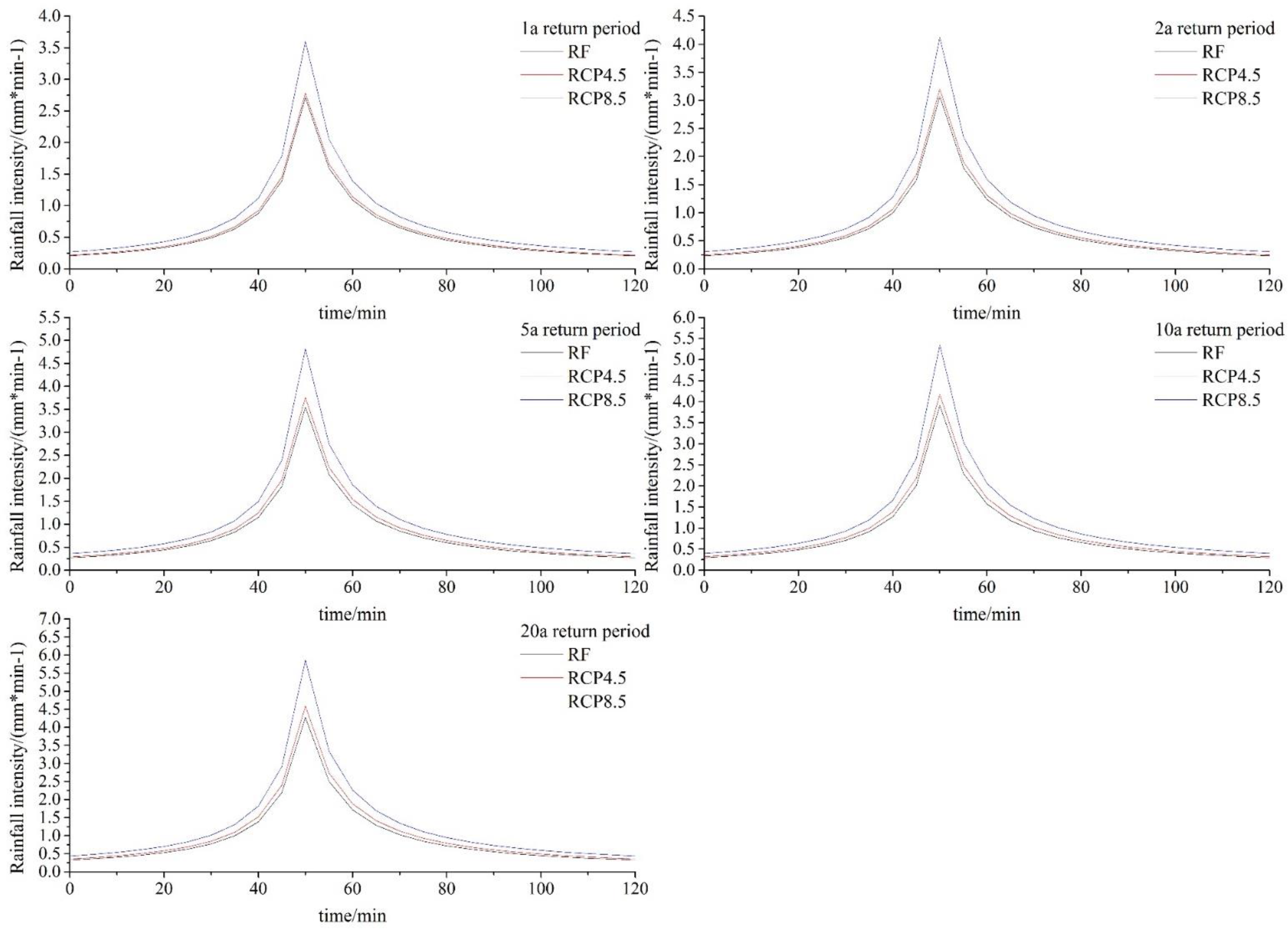
Based on the Chicago hyetograph method, Figure 2 shows the impact of climate change on the design rainstorm. The peak values increased by 0.073, 0.013, 0.205, 0.262, 0.319 mm/min from those of the reference period (RF) under scenario RCP4.5 in different return periods. The rainfall amount increased from 4.37% to 9.19% under scenario RCP4.5. The peak values under RCP8.5 significantly increased, with a maximum increase of 1.591 mm/min under the 20a return period. The amount of rainfall increased by 28.79%, 30.20%, 31.61%, 32.45%, and 33.15% in the 1a, 2a, 5a, 10a, 20a return periods, respectively. The increasing intensity of the future short-duration design rainstorm will directly impact the urban drainage system and cause more severe waterlogging issues.

4.3. Urban Flood Model Calibration and Validation

Two historical rainfalls (1 and 2) were selected as the model inputs for calibration and validation (Figure 3). The first rainfall began at 6:24 pm on 15 July 2017, and ended at 6:44 pm. The maximum intensity recorded by three rain gages was 84 mm/h, which occurred at 6:26 for Gage 1. The duration of Rainfall 1 was short, and the intensity was even lower than that of the design rainstorm with a 1a return period. The second rainfall began at 1:00 pm on 5 September 2017, and lasted for approximately 1 h. The intensity of Rainfall 2, with a peak of 5.3 mm/min, was much larger than that of Rainfall 1. Rainfall 1 caused few inundations in the research region, while Rainfall 2 caused large areas of inundations. Therefore, the junction water depth is applied to calibrate Rainfall 1, and the inundation depth is taken as the model calibration criteria for Rainfall 2.

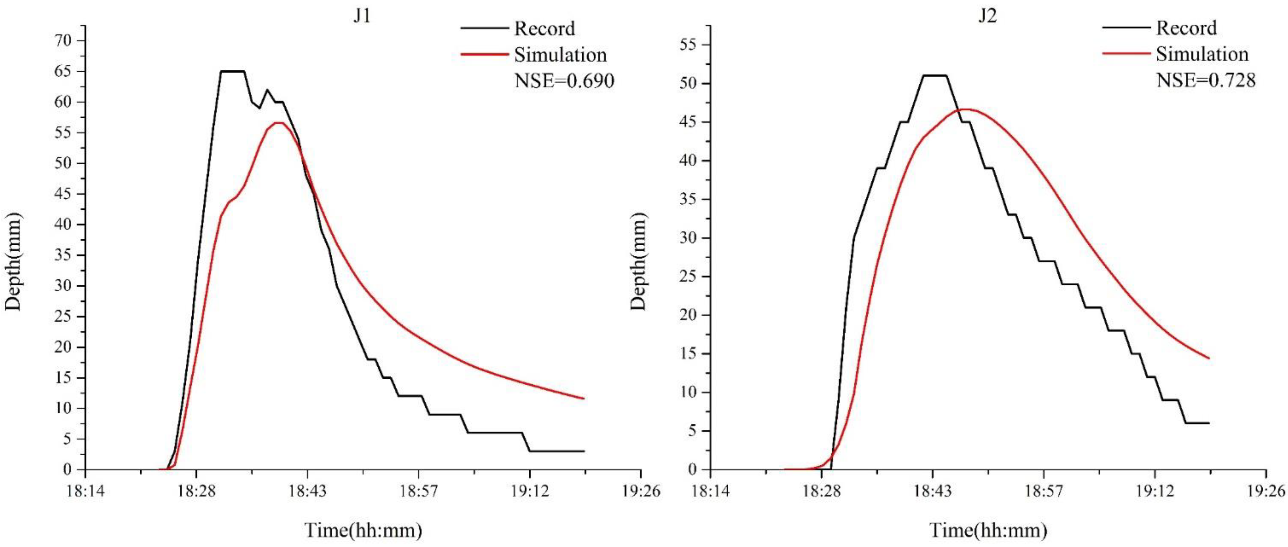
Two junctions (J1 and J2) located on the main pipelines were selected as the research objects in the calibration for Rainfall 1. The model parameters were adjusted according to the Nash–Sutcliffe efficiency coefficient (NSE) calibration method (Equation (7)), and the results are shown in Figure 4. Generally, the precision of the models is high when the NSE value exceeds 0.6. The NSE values of J1 and J2 are 0.690 and 0.728, respectively.

$$NSE=1-\frac{{\displaystyle \sum _{t-1}^T{(Q_o^t-Q_m^t)}^2}}{{\displaystyle \sum _{t=1}^T(Q_o^t-{\overline{Q}}_o)}}$$

(7)

where $Q_o^t$ is the observed value at time $t$, $Q_m^t$ is the modeled value at time $t$, and ${\overline{Q}}_o$ is the average value of the observed data throughout the total modeling time $T$.

Rainfall 2 caused severe inundations in the research region, and the inundation extents and depths are used in validation.

Table 8. Validation results between simulation depth and recorded depth.

SITE	Record Depth (m)	Simulation Depth (m)	Errors
ZZL	0.200	0.158	−0.042
HHR	0.500	0.914	0.414
BHS	0.500	0.633	0.133
DCR	0.600	0.400	−0.200
NLXR	0.500	0.427	−0.073
GFB	0.500	0.629	0.129
GMR	0.300	0.161	−0.139
HFR	0.350	0.223	−0.127
HZGH	0.400	0.481	0.081

shows a detailed comparison of the results of the maximum inundation depths with the data recorded on-site. HHR exhibits the largest error of 0.414 m, while the errors at the other sites are acceptable and do not exceed 0.2 m. In summary, this urban flood model can reproduce the historical rainfall-induced inundation after calibration and validation.

4.4. Climate Change Impact on Inundation

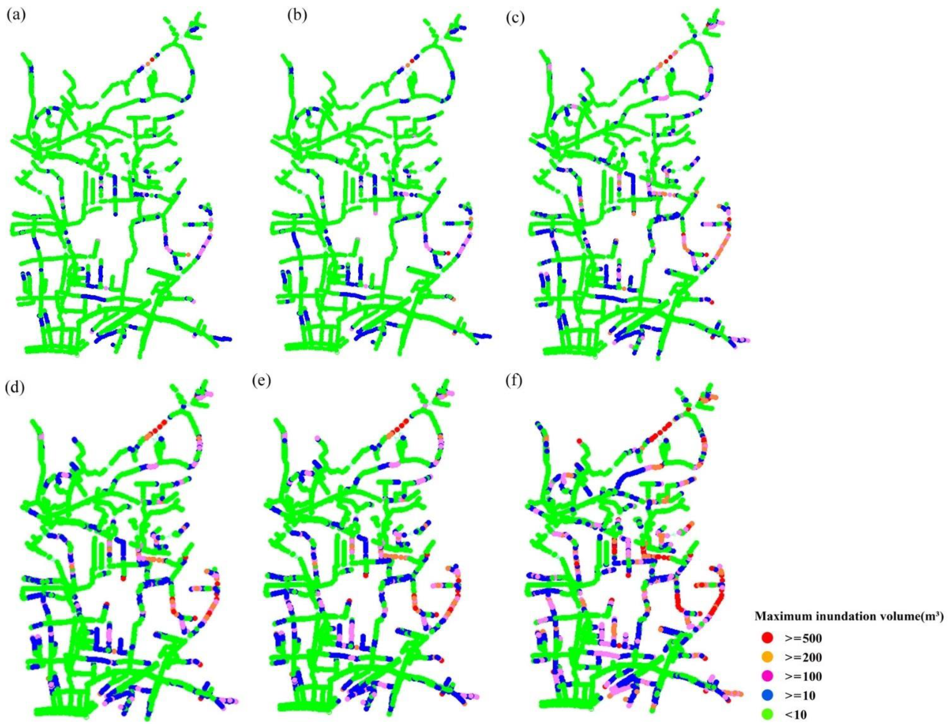
The changes in the inundation nodes under the two emission scenarios exhibited very similar patterns. Figure 5a–c show the distribution of inundation nodes in the 2a return period during the reference period, RCP4.5, and RCP8.5, respectively.

Table 9. The results of inundation node (RCP4.5 relative to RF).

Return Period	$\mathbf{Maximum} \mathbf{Node} \mathbf{Inundation} \mathbf{Volume} \left({\mathbf{m}}^3\right)$	Number of Node Inundation	Inundation Node Percentage (%)
1a	55.500	45	1.512
2a	105.300	61	2.049
5a	98.400	47	1.579
10a	104.100	46	1.545
20a	106.200	66	2.217

shows the variation in the number of inundation nodes under RCP4.5 and compares it with that of the reference period. The maximum inundation volume and inundation node are both increasing. In the 20a return period, the maximum inundation volume increased by approximately 106.2 m³, and the proportion of the inundation node increased by 2.217%.

Table 10. The results of inundation node (RCP8.5 relative to RF).

Return Period	$\mathbf{Maximum} \mathbf{Node} \mathbf{Inundation} \mathbf{Volume} \left({\mathbf{m}}^3\right)$	Number of Node Inundation	Inundation Node Percentage (%)
1a	636.700	342	11.488
2a	708.900	330	11.085
5a	742.800	386	12.966
10a	786.400	415	13.940
20a	828.700	416	13.974

shows the variation in the number of inundation nodes under RCP8.5 and compares it with that of the reference period. The inundation volume and nodes significantly increased under the RCP8.5 scenario. The maximum inundation volume increased by approximately 636.7, 708.9, 742.8, 786.4, and 828.7 m³ for each return period, respectively, and the number of inundation nodes increased by 342, 330, 386, 415, and 416 for each return period. Figure 5d–f show that the maximum inundation volume of over 100 m³ spread to the whole basin in the 20a return period under scenario RCP8.5.

Table 11. Conduit surcharge performance RCP4.5 relative RF (unit: %).

RCP4.5-RF	S < 0.5	0.5 < = S < 0.8	0.8 < = S < 1	1 < = S < 2	2 < = S
1a	−0.89	−0.82	−0.36	0.32	1.75
2a	−0.8	−0.6	−0.18	0.43	1.14
5a	−0.64	−0.27	−0.65	0.75	0.79
10a	−0.51	−0.79	0.31	−0.13	1.12
20a	−0.51	−0.54	−0.55	0.67	0.92

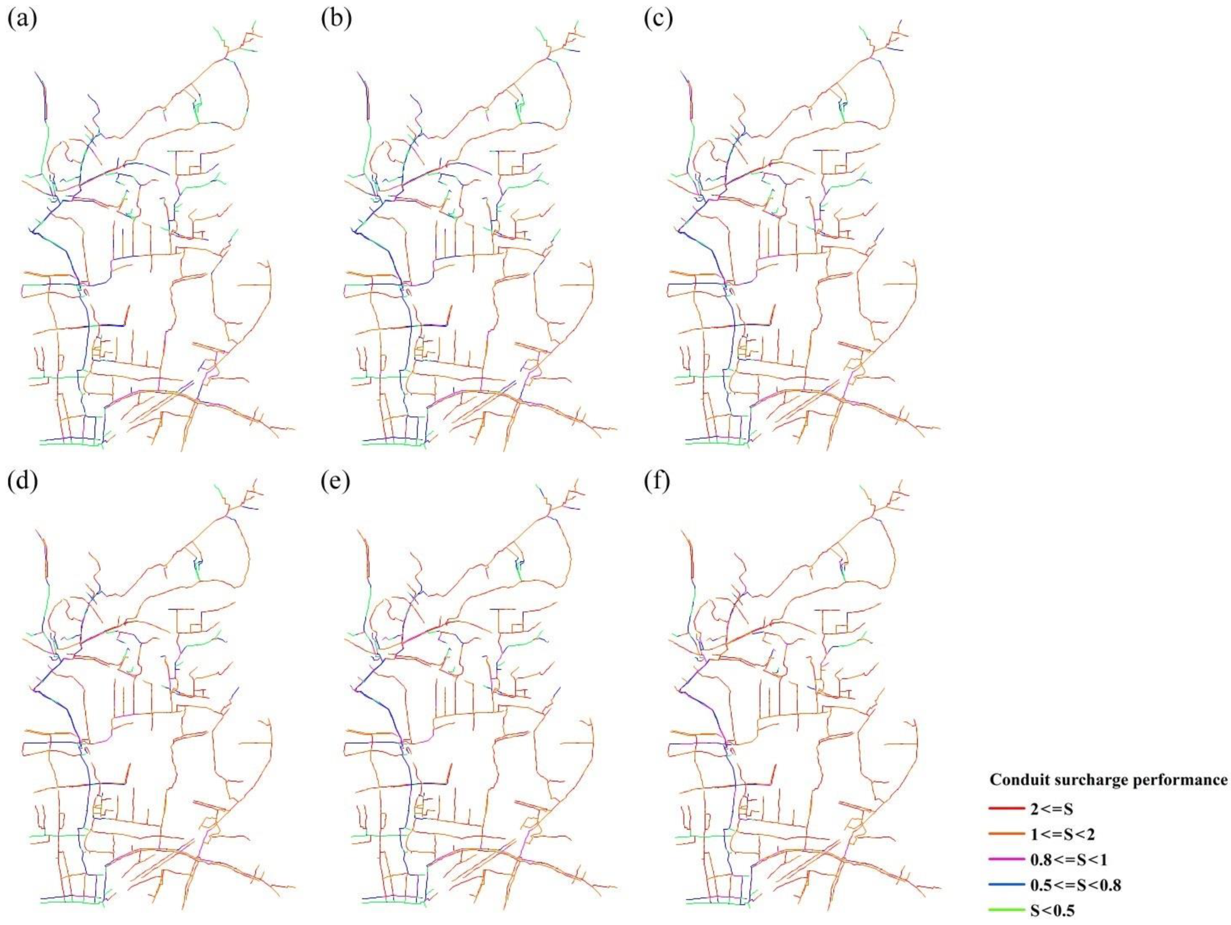
S < 0.5: conduit flow depth no more than 50%; 0.5 < = S < 0.8: conduit flow depth from 50% to 80%; 0.8 < = S < 1: conduit flow depth from 80% to 100%; 1 = < S < 2: The surcharge derive from downstream conduit flow capacity insufficient; 2 < = S: The surcharge derive from flow capacity insufficient.

shows the conduit surcharge conditions under RCP4.5 and compares them with those under the RF period. In the 1a return period, the conduit surcharge below 0.5 decreased by approximately 0.89%. The surcharge conduit proportion decreased by 0.82% and 0.6% under surcharge conditions ranging from 0.5 to 0.8 and 0.8 to 1, respectively. The proportion of full load operation increased by 2.07%, in which the proportion of conduits with full loads increased by approximately 1.75% due to the insufficient downstream flow capacity and 0.32% due to its own insufficient flow capacity. In the 20a return period, the conduit surcharge below 0.5 decreased by approximately 0.89%. The surcharge conduit proportion decreased by 0.82% and 0.6% under surcharge conditions ranging from 0.5 to 0.8 and 0.8 to 1, respectively. The proportion of full load operation increased by 1.59%, in which the proportion of conduits with full loads increased by approximately 0.92% due to the insufficient downstream flow capacity and 0.67% due to its own insufficient flow capacity.

Table 12. Conduit surcharge performance RCP8.5 relative RF (unit: %).

RCP8.5-RF	S < 0.5	0.5 < = S < 0.8	0.8 < = S < 1	1 < = S < 2	2 < = S
1a	−6.26	−4.45	−0.94	3.13	8.52
2a	−4.7	−4.4	−0.51	2	7.62
5a	−3.83	−3.95	−1.38	2.14	7.02
10a	−3.07	−3.72	−1.51	1.63	6.68
20a	−2.97	−4.51	−0.81	2.17	6.12

S < 0.5: conduit flow depth no more than 50%; 0.5 < = S < 0.8: conduit flow depth from 50% to 80%; 0.8 < = S < 1: conduit flow depth from 80% to 100%; 1 = < S < 2: The surcharge derive from downstream conduit flow capacity insufficient; 2 < = S: The surcharge derive from flow capacity insufficient.

shows the conduit surcharge conditions under RCP8.5 and compares them with those under the RF period. In the 1a return period of RCP8.5, conduit surcharges below 0.5 decreased by approximately 6.26%. The surcharge conduit proportion decreased by 4.45% and 0.94% under surcharge conditions ranging from 0.5 to 0.8 and 0.8 to 1, respectively. The proportion of full load operation increased by 11.65%, in which the proportion of conduits with full loads increased by approximately 8.52% due to the insufficient downstream flow capacity and 3.13% due to their own insufficient flow capacity. In the 20a return period, the conduit surcharge below 0.5 decreased by approximately 2.97%. The surcharge conduit proportion reduced by 4.51% and 0.81% under surcharge conditions ranging from 0.5 to 0.8 and 0.8 to 1, respectively. The proportion of full load operation increased by 8.29%, in which the proportion of conduits with full loads increased by approximately 6.12% due to the insufficient downstream flow capacity and 2.17% due to its own insufficient flow capacity. Figure 6 presents the spatial distribution of conduit surcharge conditions and compares them with the RF period; the most conduit surcharges exceed 1, which is transferred from the surcharge values of 0.8–1 and 0.5–0.8 under scenarios RCP4.5 and RCP8.5, respectively.

4.5. Climate Change Impact on Urban Waterlogging

The waterlogging distribution is shown in Figure 7, and the effect of climate change on waterlogging is investigated in this study. For further analysis, the RCP scenarios in nine typical sites of the DHC Basin are compared with the reference period.

Table 13. Changes of maximum waterlogging depth under RCP4.5 compared with RF period (unit: m).

Site	1a	2a	5a	10a	20a
ZZL	0.030	0.012	0.006	0.012	0.009
HHR	0.053	0.017	0.010	0.011	0.010
BHS	0.083	0.009	0.001	0.009	0.008
DCR	0.007	0.005	0.007	0.003	0.003
NLXR	0.064	0.049	0.041	0.033	0.034
GFB	0.062	0.009	0.003	0.004	0.005
GMR	0.052	0.039	0.033	0.037	0.051
HFR	0.057	0.015	0.001	0.005	0.004
HZGH	0.041	0.055	0.054	0.031	0.016

shows the changes in the runoff depth under RCP4.5 and compares them with the reference period. The runoff depth increased by 0.007–0.083, 0.005–0.055, 0.001–0.054, 0.003–0.037, and 0.003–0.051 m in the five return periods, respectively. The BHR site is expected to experience the largest runoff depth, with an increase of 0.083 m in the 1a return period. Under the RCP8.5 scenario, the runoff depth significantly increased at most sites.

Table 14. Changes of maximum waterlogging depth under RCP8.5 compared with RF period (unit: m).

Site	1a	2a	5a	10a	20a
ZZL	0.139	0.105	0.096	0.122	0.189
HHR	0.248	0.165	0.156	0.172	0.192
BHS	0.325	0.223	0.256	0.258	0.232
DCR	0.040	0.031	0.034	0.032	0.060
NLXR	0.369	0.314	0.253	0.242	0.247
GFB	0.210	0.031	0.020	0.023	0.024
GMR	0.305	0.269	0.290	0.307	0.314
HFR	0.117	0.051	0.032	0.029	0.030
HZGH	0.349	0.376	0.215	0.112	0.084

shows the changes in runoff depth under the RCP8.5 scenario relative to those of the reference period. The maximum runoff depth increased by 0.369, 0.314, 0.290, 0.307, and 0.314 m in five return periods, respectively. The maximum change in the runoff depth can be observed at NLR in the 1a return period, while the smallest increase can be observed at GMR, with an increase of 0.020 m in the 5a return period.

Table 15. Changes of submerged area (unit: %).

Scenario	1a	2a	5a	10a	20a
RCP4.5-RF	5.53	5.21	5.09	10.49	4.67
RCP8.5-RF	47.06	41.84	40.51	43.07	31.5

shows the variation in the submerged area. Under scenario RCP4.5, the changes in the submerged area increased by 5.53%, 5.21%, 5.09%, 10.49%, 4.67% in the five return periods. The largest change in the submerged area can be observed in the 10a return period, with an increase of 179,500 m². Under scenario RCP8.5, the submerged area is remarkably dispersed in the study area. The changes in the submerged area increased by 47.06%, 41.84%, 40.51%, 43.07%, and 31.50% in the five return periods. The maximum change in the submerged area can be observed in the 10a return period with an increase of 736,700 m².

5. Discussion

This study was conducted to explore the effect of climate change on urban drainage systems, based on two RCP scenarios. Overall, urban inundation and waterlogging will become more intense in the future, which is somewhat consistent with previous findings for urban areas [25,27,47]. We also found that the increase in the intensity of inundation and waterlogging is expected to be more pronounced under the high-emissions scenario (RCP8.5) than those under the moderate-emissions scenario (RCP4.5). Therefore, this study illustrates that the current urban drainage system will cause more austere urban waterlogging. The design of urban drainage systems needs to consider more complex environmental and adverse conditions.

Generally, GCM and emission scenarios are considered to be the greatest sources of uncertainty in relation to climate change, especially for extreme climate events [48,49]. The validation of the climate model simulation suggested that the RegCM4.6 can reasonably reproduce the variability of monthly precipitation and extreme precipitation events compared with the observations. However, it should be emphasized that some discrepancies were still detected between the simulations and observations, suggesting that there is an uncertainty in the projection of future flooding risk. Generally, GCM and emission scenarios are considered to be the largest sources of uncertainty in relation to climate change, especially for extreme climate events. We used only RCM driven by one GCM, which may limit the scope of this study and there exist further uncertainties associated with projections of future precipitation and climate extremes. Further studies are required to be focused on different GCMs and emissions scenarios toward a more reliable projection of climate change. Further studies are required to investigate these, using different methods for downscaling the projections (such as dynamic and statistical downscaling) and different GCMs and emission scenarios to drive the simulations. Therefore, effectively using multiple models when applying downscaling techniques with more confidence should be considered in future research. By comparing the results of different simulations, we can improve our understanding of some of the uncertainties associated with climate change, and a consistent timescale will be applied to further detect the impact of climate change on urban drainage systems.

Integrating the delta change and annual maximum value methods to derive a design rainstorm is a new research area for understanding the impact of climate change on the urban drainage system. Unlike previous studies, which mainly focus on hourly rainfall derived by a climate model that is associated with great uncertainty [25], this method mainly focused on short-duration design rainfall, which could aid the design of future sophisticated urban drainage systems. However, it should be emphasized that, based on the theory of the delta method, the selection of a timescale between delta change and annual maximum value methods is neglected when developing the design formula. This could result in some discrepancies in the derivation of design rainfall. In future investigations, the annual maximum rainstorm factor for each timescale should be consistent with that of the delta factor. The different applicable distribution analysis is partly overlooked in this study. Next step, the different distribution should be incorporated in the curve fitting to explore the effects of applicable distribution. By comparing the results of different simulations and curve fitting, the derivation of a design rainstorm will be more reasonable.

6. Conclusions

In this study, the reference urban drainage system of and future inundation and waterlogging in the DHC Basin were investigated using the output of the delta change method by GFDL-ESM-2M. The future design rainfall is derived and then integrated with InfoWorks ICM to evaluate the urban inundation and waterlogging risk. The main findings can be summarized as follows:

The delta change and annual maximum value methods were integrated to determine the future urban design rainfall under RCP4.5 and RCP8.5 scenarios. Pearson-3 type curve and parameter optimization were applied to determine the future design rainfall formula. This method offers a new insight to aid in managing the effect of climate change on urban areas. Compared to the reference period with the Chicago hyetograph method, the peak value and amount of rainfall increased under the RCP4.5 and RCP8.5 scenarios, indicating that the urban drainage system will face more austere urban flood control pressure.

The InfoWorks ICM model was used to evaluate the variations in urban inundation. Compared to the reference period, the number of inundation nodes and inundation volume were increasing in all five return periods in the DHC Basin under scenarios RCP4.5 and RCP8.5. Their increase was more significant under RCP8.5 than that under RCP4.5. The variation in inundation was most severe under the 20a return period. The conduit surcharge conditions showed that the proportion of fully loaded conduits increased in all return periods. The largest percentage increase in the proportion of fully loaded conduits could be observed in the 1a return period. Transformation of the conduit network should be considered under multiple return periods.

The 2-D model was implemented to evaluate the changes in waterlogging. Nine typical waterlogging sites in the DHC Basin were selected to measure the variations in runoff depth. Compared to the reference period, the runoff depth increased in nine sites during all return periods. The increases under RCP8.5 were more significant than those under RCP4.5 scenarios. Throughout the basin, the increase in the submerged area did not exceed 15% under RCP4.5, but it exceeded 30% under scenario RCP8.5.

References

1. IPCC. Summary for Policymakers. In Climate Change 2013: The Physical Science Basis. Contribution of Working Group I to the Fifth Assessment Report of the Intergovernmental Panel on Climate Change; Cambridge University Press: Cambridge, UK; New York, NY, USA, 2013. [Google Scholar]
2. Karamouz, M.; Hosseinpour, A.; Nazif, S. Improvement of Urban Drainage System Performance under Climate Change Impact: Case Study. J. Hydraul. Eng. 2011, 16, 395–412. [Google Scholar] [CrossRef]
3. Cuo, L.; Beyene, T.K.; Voisin, N.; Su, F.; Lettenmaier, D.P.; Alberti, M.; Richey, J.E. Effects of mid-twenty-first century climate and land cover change on the hydrology of the Puget Sound basin, Washington. Hydrol. Processes 2011, 25, 1729–1753. [Google Scholar] [CrossRef]
4. Kay, A.L.; Jones, D.A. Transient changes in flood frequency and timing in Britain under potential projections of climate change. Int. J. Climatol. 2012, 32, 489–502. [Google Scholar] [CrossRef] [Green Version]
5. Liu, S.; Gao, W.; Liang, X.-Z. A regional climate model downscaling projection of China future climate change. Clim. Dynam. 2013, 41, 1871–1884. [Google Scholar] [CrossRef]
6. Zhou, T.; Li, Z. Simulation of the east asian summer monsoon using a variable resolution atmospheric GCM. Clim. Dynam. 2002, 19, 167–180. [Google Scholar]
7. Giorgi, F.; Shields, C. Tests of precipitation parameterizations available in latest version of NCAR regional climate model (RegCM) over continental United States. J. Geophys. Res. Atmos. 1999, 104, 6353–6375. [Google Scholar] [CrossRef]
8. Gao, X.; Pal Jeremy, S.; Giorgi, F. Projected changes in mean and extreme precipitation over the Mediterranean region from a high resolution double nested RCM simulation. Geophys. Res. Lett. 2006, 33, L03706. [Google Scholar] [CrossRef]
9. Ji, Z.; Kang, S. Evaluation of extreme climate events using a regional climate model for China. Int. J. Climatol. 2015, 35, 888–902. [Google Scholar] [CrossRef]
10. Wu, C.; Huang, G. Changes in heavy precipitation and floods in the upstream of the Beijiang River basin, South China. Int. J. Climatol. 2015a, 35, 2978–2992. [Google Scholar] [CrossRef]
11. Chen, Z.; Yin, L.; Chen, X.; Wei, S.; Zhu, Z. Research on the characteristics of urban rainstorm pattern in the humid area of Southern China: A case study of Guangzhou City. Int. J. Climatol. 2015, 35, 4370–4386. [Google Scholar] [CrossRef]
12. Wu, X.; Guo, S.; Yin, J.; Yang, G.; Zhong, Y.; Liu, D. On the event-based extreme precipitation across China: Time distribution patterns, trends, and return levels. J. Hydrol. 2018, 562, 305–317. [Google Scholar] [CrossRef]
13. Fu, G.; Butler, D.; Khu, S.-T.; Sun, S.A. Imprecise probabilistic evaluation of sewer flooding in urban drainage systems using random set theory. Water Resour. Res. 2011, 47, W02534. [Google Scholar] [CrossRef] [Green Version]
14. Zhu, Z.; Chen, Z.; Chen, X.; He, P. Approach for evaluating inundation risks in urban drainage systems. Sci. Total Environ. 2016, 553, 1–12. [Google Scholar] [CrossRef]
15. Yu, M.; Liu, Y. The possible impact of urbanization on a heavy rainfall event in Beijing. J. Geophys. Res. Atmos. 2015, 120, 8132–8143. [Google Scholar] [CrossRef]
16. Coumou, D.; Rahmstorf, S. A decade of weather extremes. Nat. Clim. Chang. 2012, 2, 491–496. [Google Scholar] [CrossRef]
17. Zhang, D.; Lin, Y.; Zhao, P.; Yu, X.; Wang, S.; Kang, H.; Ding, Y. The Beijing extreme rainfall of 21 July 2012: “Right results” but for wrong reasons. Geophys. Res. Lett. 2013, 40, 1426–1431. [Google Scholar] [CrossRef]
18. Cameron, D. An application of the UKCIP02 climate change scenarios to flood estimation by continuous simulation for a gauged catchment in the northeast of Scotland, UK (with uncertainty). J. Hydrol. 2006, 328, 212–226. [Google Scholar] [CrossRef]
19. Semadeni-Davies, A.; Hernebring, C.; Svensson, G.; Gustafsson, L.-G. The impacts of climate change and urbanisation on drainage in Helsingborg, Sweden: Suburban stormwater. J. Hydrol. 2008, 350, 114–125. [Google Scholar] [CrossRef]
20. Zhou, Q.; Mikkelsen, P.S.; Halsnæs, K.; Arnbjerg-Nielsen, K. Framework for economic pluvial flood risk assessment considering climate change effects and adaptation benefits. J. Hydrol. 2012, 414–415, 539–549. [Google Scholar] [CrossRef]
21. Wu, X.; Wang, Z.; Guo, S.; Liao, W.; Zeng, Z.; Chen, X. Scenario-based projections of future urban inundation within a coupled hydrodynamic model framework: A case study in Dongguan City, China. J. Hydrol. 2017, 547, 428–442. [Google Scholar] [CrossRef]
22. Chen, W.; Huang, G.R.; Zhang, H.; Wang, W. Urban inundation response to rainstorm patterns with a coupled hydrodynamic model: A case study in Haidian Island, China. J. Hydrol. 2018, 564, 1022–1035. [Google Scholar] [CrossRef]
23. Wernstedt, K.; Carlet, F. Climate Change, Urban Development, and Storm Water: Perspectives from the Field. J. Water Resour. Plan. Manag. 2014, 140, 543–552. [Google Scholar] [CrossRef]
24. IPCC. Summary for Policymakers. In Climate Change 2007: The Physical Science Basis. Contribution of Working Group I to the Fourth Assessment Report of the Intergovernmental Panel on Climate Change; Cambridge University Press: Cambridge, UK; New York, NY, USA, 2007. [Google Scholar]
25. Berggren, K.; Olofsson, M.; Viklander, M.; Svensson, G.; Gustafsson, A.-M. Hydraulic Impacts on Urban Drainage Systems due to Changes in Rainfall Caused by Climatic Change. J. Hydraul. Eng. 2012, 17, 92–98. [Google Scholar] [CrossRef]
26. Anandhi, A.; Frei, A.; Pierson, D.C.; Schneiderman, E.M.; Zion, M.S.; Lounsbury, D.; Matonse, A.H. Examination of change factor methodologies for climate change impact assessment. Water Resour. Res. 2011, 47, W03501. [Google Scholar] [CrossRef] [Green Version]
27. Zahmatkesh, Z.; Karamouz, M.; Goharian, E.; Burian, S.J. Analysis of the Effects of Climate Change on Urban Storm Water Runoff Using Statistically Downscaled Precipitation Data and a Change Factor Approach. J. Hydraul. Eng. 2015, 20, 05014022. [Google Scholar] [CrossRef]
28. Olsson, J.; Berggren, K.; Olofsson, M.; Viklander, M. Applying climate model precipitation scenarios for urban hydrological assessment: A case study in Kalmar City, Sweden. Atmos. Res. 2009, 92, 364–375. [Google Scholar] [CrossRef]
29. Wu, H.; Huang, G.; Meng, Q.; Zhang, M.; Li, L. Deep Tunnel for Regulating Combined Sewer Overflow Pollution and Flood Disaster: A Case Study in Guangzhou City, China. Water 2016, 8, 329. [Google Scholar] [CrossRef] [Green Version]
30. Zhang, M.; Zeng, J.; Huang, G.R.; Liu, H. Analysis of cohesive relationship for return period of design rainstorm between municipal sewerage and waterlogging drainage. J. Water Res. Water Eng. 2015, 26, 131–135. [Google Scholar]
31. Wan, Y.; Ye, X.; Wang, F.; Liu, J.; Li, D. Study on the formula of deducing heavy rain intensity by different fitting methods. J. Water Res. Water Eng. 2017, 28, 76–79+86. [Google Scholar]
32. Mei, C.; Liu, J.; Wang, H.; Xiang, C.; Zhou, J. Review on urban design rainstorm. Chin. Sci. Bull. 2017, 62, 3873–3884. [Google Scholar] [CrossRef] [Green Version]
33. Dai, Y.; Wang, Z.; Dai, L.; Cao, Q.; Wang, T. Application of Chicago Hyetograph Method in Design of Short Duration Rainstorm Pattern. J. Arid Meteor. 2017, 35, 1061–1069. [Google Scholar]
34. Keifer, C.J.; Chu, H.H. Synthetic storm pattern for drainage design. J. Hydraul. Div. 1957, 83, 1–25. [Google Scholar]
35. Grell, G.A. Prognostic Evaluation of Assumptions Used by Cumulus Parameterizations. Mon. Weather Rev. 1993, 121, 764–787. [Google Scholar] [CrossRef] [Green Version]
36. Kiehl, J.; Hack, J.; Bonan, G.; Boville, B.; Briegleb, B.; Williamson, D.; Rasch, P. Description of the NCAR community climate model (CCM3); NCAR Technical Note NCAR/TN-420 STR: Boulder, CO, USA, 1996; p. 152. [Google Scholar]
37. Dickinson, R.; Henderson-Sellers, A.; Kennedy, P. Biosphere-Atmosphere Transfer Scheme (BATS) Version 1 as Coupled to the NCAR Community Climate Model; NCAR Technical Note NCAR/TN-387 STR: Boulder, CO, USA, 1993; p. 72. [Google Scholar]
38. Holtslag, A.A.M.; De Bruijn, E.I.F.; Pan, H.L. A High Resolution Air Mass Transformation Model for Short-Range Weather Forecasting. Mon. Weather Rev. 1990, 118, 1561–1575. [Google Scholar] [CrossRef]
39. Zeng, X.; Zhao, M.; Dickinson, R.E. Intercomparison of Bulk Aerodynamic Algorithms for the Computation of Sea Surface Fluxes Using TOGA COARE and TAO Data. J. Clim. 1998, 11, 2628–2644. [Google Scholar] [CrossRef]
40. Arakawa, A.; Schubert, W.H. Interaction of a Cumulus Cloud Ensemble with the Large-Scale Environment, Part I. J. Atmos. Sci. 1974, 31, 674–701. [Google Scholar] [CrossRef] [Green Version]
41. Dunne, J.P.; John, J.G.; Adcroft, A.J.; Griffies, S.M.; Hallberg, R.W.; Shevliakova, E.; Stouffer, R.J.; Cooke, W.; Dunne, K.A.; Harrison, M.J.; et al. GFDL’s ESM2 Global Coupled Climate–Carbon Earth System Models. Part I: Physical Formulation and Baseline Simulation Characteristics. J. Clim. 2012, 25, 6646–6665. [Google Scholar] [CrossRef] [Green Version]
42. Dunne, J.P.; John, J.G.; Shevliakova, E.; Stouffer, R.J.; Krasting, J.P.; Malyshev, S.L.; Milly, P.C.D.; Sentman, L.T.; Adcroft, A.J.; Cooke, W.; et al. GFDL’s ESM2 Global Coupled Climate–Carbon Earth System Models. Part II: Carbon System Formulation and Baseline Simulation Characteristics. J. Clim. 2012, 26, 2247–2267. [Google Scholar] [CrossRef] [Green Version]
43. Loveland, T.R.; Reed, B.C.; Brown, J.F.; Ohlen, D.O.; Zhu, Z.; Yang, L.; Merchant, J.W. Development of a global land cover characteristics database and IGBP DISCover from 1 km AVHRR data. Int. J. Remote Sens. 2010, 21, 1303–1330. [Google Scholar] [CrossRef]
44. Bruen, M.; Yang, J. Combined Hydraulic and Black-Box Models for Flood Forecasting in Urban Drainage Systems. J. Hydraul. Eng. 2006, 11, 589–596. [Google Scholar] [CrossRef]
45. Cheng, T.; Xu, Z.; Song, S. Rainfall-runoff simulations for Xinglong sponge city pilot area of Jinan. J. Hydraul. Eng. 2017, 35, 1–11. [Google Scholar]
46. Huang, G.; Wang, X.; Huang, W. Simulation of Rainstorm Waterlogging in the Urban Area Based on InfoWorks ICM model. Water Resour. Pow. 2017, 35, 66–70+60. [Google Scholar]
47. Karamouz, M.; Nazif, S. Reliability-Based Flood Management in Urban Watersheds Considering Climate Change Impacts. J. Water Res. Plan. Man. 2013, 139, 520–533. [Google Scholar] [CrossRef]
48. Kay, A.L.; Davies, H.N.; Bell, V.A.; Jones, R.G. Comparison of uncertainty sources for climate change impacts: Flood frequency in England. Clim. Chang. 2008, 92, 41–63. [Google Scholar] [CrossRef]
49. Wu, C.H.; Huang, G.R.; Yu, H.J. Prediction of extreme floods based on CMIP5 climate models: A case study in the Beijiang River basin, South China. Hydrol. Earth Syst. Sci. 2015b, 19, 1385–1399. [Google Scholar] [CrossRef] [Green Version]
Figure 1. Location of the DongHaoChong basin and the spatial distribution of main waterlogging sites. ZZL, Zhuziliao; HHR, Huanghua Road; BHS, Beiheng Street; DCR, Dongchuan Road; NLXR, Nonglinxia Road; GFB, Guangfa Bank; GMR, Guangming Road; HFR, Hengfu Road; HZGH, Hengzhigang Hospital.
Water 13 02718 g001
Figure 2. The Chicago hyetograph shapes of rainstorm lasting 120min with different return periods under RF, RCP4.5, RCP8.5 scenarios.
Water 13 02718 g002
Figure 3. Hydrographs of the two historical rainfall 1 and rainfall 2.
Water 13 02718 g003
Figure 4. Calibrated junction water depths (J1 and J2).
Water 13 02718 g004
Figure 5. The spatial distribution of inundation nodes. (a) 2a return period under RF period. (b) 2a return period under RCP4.5. (c) 2a return period under RCP8.5. (d) 20a return period under RF period. (e) 20a return period under RCP4.5. (f) 20a return period under RCP8.5.
Water 13 02718 g005
Figure 6. The spatial distribution of conduit surcharge performance. (a) 2a return period under RF period. (b) 2a return period under RCP4.5. (c) 2a return period under RCP8.5. (d) 20a return period under RF period. (e) 20a return period under RCP4.5. (f) 20a return period under RCP8.5.
Water 13 02718 g006
Figure 7. The spatial distribution of waterlogging depth. (a) 2a return period under RF period. (b) 2a return period under RCP4.5. (c) 2a return period under RCP8.5. (d) 20a return period under RF period. (e) 20a return period under RCP4.5. (f) 20a return period under RCP8.5.
Water 13 02718 g007