Abstract
Reasonable optimal operation policy for complex multiple reservoir systems is very important for the safe and efficient utilization of water resources. The operation policy of multiple hydropower reservoirs should be optimized to maximize total hydropower generation, while ensuring flood control safety by effective and efficient storage and release policy of multiple reservoirs. To achieve this goal, a new meta-heuristic algorithm, salp swarm algorithm (SSA), is used to optimize the joint operation of multiple hydropower reservoirs for the first time. SSA is a competitive bio-inspired optimizer, which has received substantial attention from researchers in a wide variety of applications in finance, engineering, and science because of its little controlling parameters and adaptive exploratory behavior. However, it still faces few drawbacks such as lack of exploitation and local optima stagnation, leading to a slow convergence rate. In order to tackle these problems, multiple strategies combining sine cosine operator, opposition-based learning mechanism, and elitism strategy are applied to the original SSA. The sine cosine operator is applied to balance the exploration and exploitation over the course of iteration; the opposition-based learning mechanism is used to enhance the diversity of the swarm; and the elitism strategy is adopted to find global optima. Then, the improved SSA (ISSA) is compared with six well-known meta-heuristic algorithms on 23 classical benchmark functions. The results obtained demonstrate that ISSA outperforms most of the well-known algorithms. Then, ISSA is applied to optimal operation of multiple hydropower reservoirs in the real world. A multiple reservoir system, namely Xiluodu Reservoir and Xiangjiaba Rservoir, in the upper Yangtze River of China are selected as a case study. The results obtained show that the ISSA is able to solve a real-world optimization problem with complex constraints. In addition, for the typical flood with a 100 return period in 1954, the maximum hydropower generation of multiple hydropower reservoirs is about 6671 GWh in the case of completing the flood control task, increasing by 1.18% and 1.77% than SSA and Particle Swarm Optimization (PSO), respectively. Thus, ISSA can be used as an alternative effective and efficient tool for the complex optimization of multiple hydropower reservoirs. The water resources in the river basin can be further utilized by the proposed method to cope with the increasingly serious climate change.
1. Introduction
With construction of new large-scale water storage projects in China and other countries all over the world, attention gradually focuses on improving the operational effectiveness and efficiency of existing reservoir systems for maximizing the beneficial uses of these projects [1,2]. Over the past few decades, a large number of hydraulic projects have been built and put into operation, which substantially promote the development and utilization of water resources [3,4]. Optimizing the utilization of reservoirs has become an indispensable part of water resources planning [5,6]. At the same time, electricity demand is substantially improved because of the increasing standards of living, industrialization, and growing populations [7,8]. This increased demand has brought more concerns about the sustainable supply and development of water resources and the maximum of economic benefits of hydropower reservoirs because the hydropower is one of the most important clean energies [9,10]. However, it is well known that most of the reservoirs serve multiple purposes for hydropower generation, flood control, and other functions of water consumption [11,12]. From the perspective of flood control, floods are devastating natural disasters globally, which are growing more intense and frequent around the world because of the changing climate and anthropogenic activities [13]. According to preliminary statistics, devastating flood incidents have caused a huge number of deaths and enormous property loss across the world, bringing great challenges to human life and production [14]. In other words, reservoirs with flood control functions must ensure the safety of downstream protected regions and reservoirs themselves during a flood event [15]. As a result, the formulation of operation policy balancing hydropower generation and flood control for multiple reservoir systems is particularly important and necessary [16,17,18].
Optimal operation of a multiple reservoir system is a complex decision-making process with multiple objectives and a number of nonlinear constraints including equality, inequality, and bound constraints [19,20]. At present, some scholars at home and abroad have carried out a number of studies on the optimal operation of multi-purpose reservoirs, including flood control, hydropower generation, water supply, navigation, ecology, and so on. In general, most of the multi-purpose reservoirs serve hydropower generation and flood control as key purposes [21,22]. The methods have been used to handle multiple objectives include weighing approach, the constraint method, and meta-heuristic optimization techniques [19]. The last one is the most popular approach because of its simplicity, flexibility, derivation-free mechanism, and local optima avoidance [23]. Zhou et al. applied a non-dominated sorting genetic algorithm (NSGA-II) to efficiently counterbalance the risks of flood control and hydropower generation in the dynamic operation of multiple hydropower reservoirs [24]. Rahimi et al. employed an imperialist competitive algorithm (ICA) to optimize multi-reservoir utilization operation for overcoming the conflict between the flood control and the revenue generated from hydropower energy [25]. However, the multi-objective optimization for flood control and hydropower generation may decrease the social and economic benefit of multiple reservoir systems because of the decision-making difficulties caused by the Pareto optimal solution sets.
Rational and judicious operation of multiple hydropower reservoirs is vital and critical during the flood season [26,27,28]. The optimal allocation of flood control capacity upstream determines the flood control safety downstream to a certain extent. An optimal operation policy simultaneously considering hydropower generation and flood control to achieve the optimal allocation of flood control capacity for a decision maker is urgently needed. The best solution is to maximize the hydropower generation and also meet the requirements of storage and release water for any particular flood event. For example, upstream reservoirs usually need to intercept a certain amount of flood volume to cooperate with a downstream reservoir to complete flood control tasks. In this case, how to maximize the benefits of hydropower generation for multiple hydropower reservoirs is a very challenging problem. To solve this challenging problem, the key variable to control the operation scheme of multiple hydropower reservoirs is the available flood storage capacity. Therefore, a new storage and release policy integrating the interception demand of certain flood volume in flood season into optimal operation of multiple hydropower reservoirs is proposed to maximize the hydropower generation considering flood control requirement simultaneously; then, a new bio-inspired optimizer (Salp Swarm algorithm, SSA for short) enhanced by multiple strategies is applied to solve the optimization problem of a multiple reservoir system.
In recent years, meta-heuristic algorithms have been widely used to tackle optimization problems in different fields such as science, engineering, and industry [29]. Assuming an optimization problem as a black box only needs an input and then gives an output without derivative calculation of the search space. Evolutionary and swarm intelligence techniques are the two important branches of meta-heuristic algorithms [30,31]. The state-of-the-art in the field of meta-heuristic algorithms are Particle Swarm Optimization (PSO) [32], Grey Wolf Optimizer (GWO) [23], Whale Optimization Algorithm (WOA) [33], Artificial Bee Colony (ABC) algorithm [34], Sine Cosine Algorithm (SCA) [35], SSA [36], and so on. Among them, SSA is a highly competitive algorithm based on the information sharing and exchange technique of salp swarm in the ocean as search agents and is found to be highly effective because of its little controlling parameters and adaptive exploratory behavior. However, for all we know, few literature works have applied SSA to tackle the optimal operation problem of multiple hydropower reservoirs so far. To refill this research gap, SSA is introduced in this paper for reservoir optimal operation for the first time. However, it is noteworthy that no single intelligence algorithms are able to solve all optimization problems [23]. This means that the success of an algorithm in solving a specific set of problems does not guarantee solving all optimization problems with different type and nature. In other words, all of the optimization techniques perform equally on average when considering all optimization problems despite the superior performance on a subset of optimization problems [37]. Thus, the original SSA was found to suffer from few drawbacks such as slow convergence rate and stagnation in local optima during the application process. To overcome the drawbacks faced by the original SSA for optimal operation of multiple reservoir system, an improved SSA (ISSA) algorithm is proposed by integrating the sine cosine operator (SCO) [35], opposition-based learning (OBL) mechanism [38], and elitism strategy into the original SSA. To the best of our knowledge, these strategies are first adopted to promote the efficiency of the original SSA by equipping it with multiple strategies. The SCO is applied to find trade-offs between exploration and exploitation; the OBL is used to enrich the diversity of salp swam over the course of iterations; the elitism strategy is adopted to select the global solution, and a modified updating mechanism of a search agent is proposed. Then, the ISSA is applied to the optimal operation of multiple hydropower reservoirs to increase the hydropower generation under the condition of guaranteeing the flood control demand of the river basin.
The rest of the paper is organized below: the optimal operation model of multiple hydropower reservoirs is established in Section 2. The overview of the original SSA and multiple strategies is given in Section 3. In Section 4, a new improved version of SSA is proposed using multiple strategies including SCO, OBL, and elitism selection strategy. Performance of the ISSA algorithm in benchmark functions is verified in Section 5. Application of ISSA for optimal operation of multiple reservoir system is described in detail in Section 6. Conclusions and the future directions are drawn in Section 7.
2. Optimal Operation Model of the Multiple Reservoir System
2.1. Objectives
In this study, the objective of the multiple reservoir system is maximization of total hydropower generation, which can be expressed below:
where E is the total hydropower generation produced during operation periods; Pi,t, ki,t, Hi,t, and Qi,t are the power output, power production coefficient, water head, and turbine discharge of reservoir i at period t, respectively; is the operation interval.
2.2. Constraints
The optimal operation of multiple reservoir system is a complex constrained optimization problem [39]. The multiple constraints are expressed below:
- (1)
- Water balance equations
- (2)
- Water head equations
- (3)
- Forebay water level limits
- (4)
- Forebay water level fluctuation limits
- (5)
- Turbine discharge limits
- (6)
- Total discharge limits
- (7)
- Power output limits
- (8)
- Total power output limits
- (9)
- Initial and target forebay water level limits
- (10)
- Nonlinear characteristic curves limits
- (11)
- Storage and release water limits
2.3. Constraints Handling Method
A constraint handling method is equipped with ISSA to cope with complex constraints for multiple reservoir systems. The constraints mentioned above can be divided into three types. One is water level limits, the second is discharge limits, and another is output limits. Three limits correspond to water level sets S1, S2, and S3, respectively. A death penalty function is used to penalize the search agents with a very large objective value in case of violation of any constraints at any level. The constraints handling method is expressed below:
(1) Transform discharge and output limits into water level limits and ;
(2) Take the intersection S of S1, , and obtained;
It is noteworthy that the priority of water level limit is higher than discharge limit and output limit. Thus, the water level limit is given priority when the intersection S is null.
(3) Calculate total violation of each search agent, which can be expressed below:
where and are the violation of discharge and output of each search agent at period t, respectively.
It is noteworthy that the upstream water levels of reservoir are selected as decision variables in the present study.
3. Background of SSA and Multiple Strategies
3.1. Original Salp Swarm Algorithm
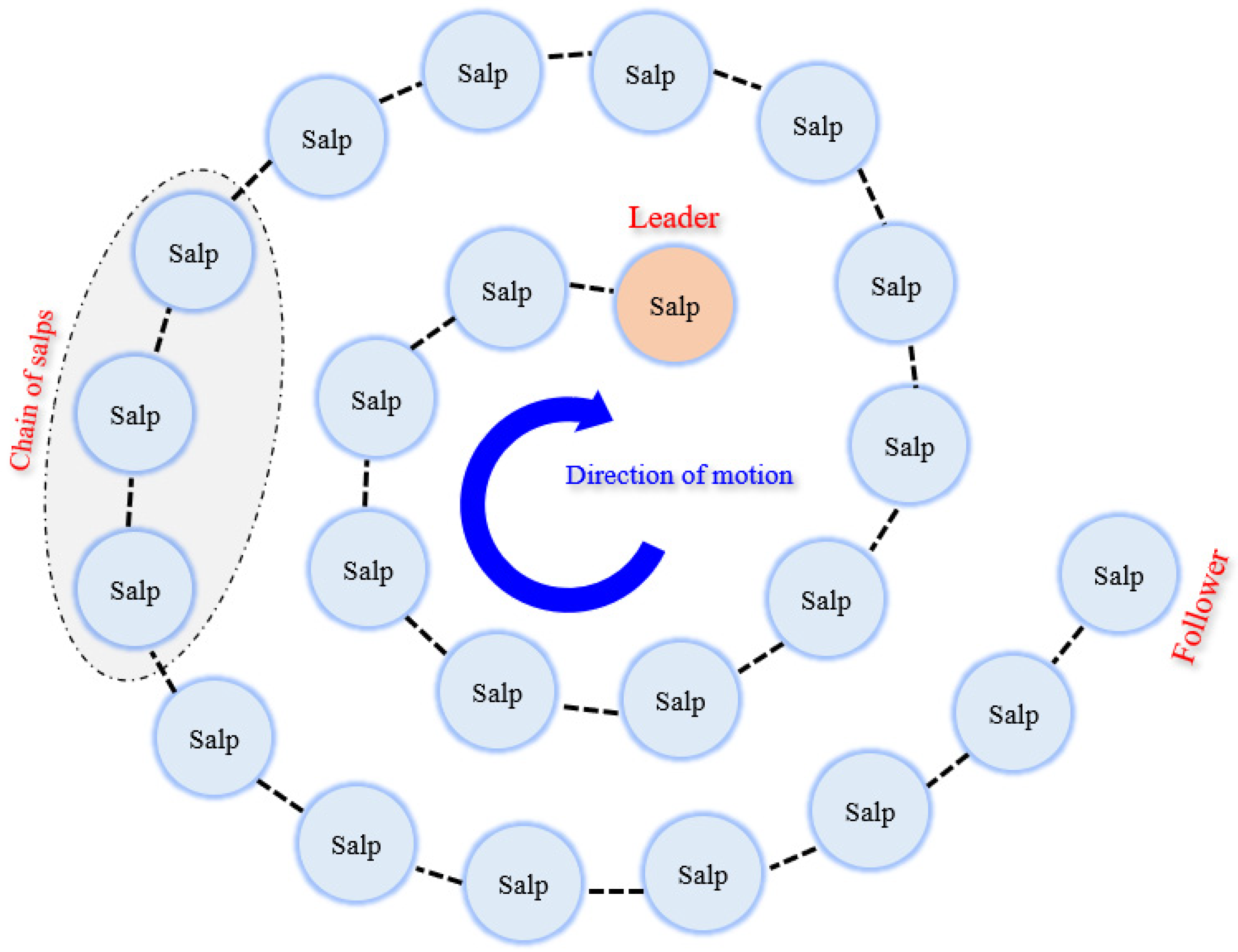
SSA is proposed to simulate the social behavior such as navigation and foragng of salp swarms, which has been proved as an alternative tool for optimization problems in different fields [36]. Salp is a barrel-shaped, planktic tunicate, which moves by contracting to pump water through its gelatinous body. The movement of salp is one of the most efficient examples of jet propulsion in the animal kingdom [40]. The life cycle of salps is complex with obligatory alternation of generations, including solitary life history phase and aggregation phase.
The SSA algorithm is mainly developed to model the swarming and foraging behavior of salp chains formed during the aggregate phase. Figure 1 shows the natural behavior of salp swarm, indicating that most of the salps follow the first salp in the chain in a certain order. Inspired by this aggregation behavior, the swarm in the salp chain can be divided into two types including leader and followers. The salp chain is arranged in order under the leader, but the order of the single salp varies over living and feeding together in the sea. For the sake of easy understanding, the global optimal solution is regarded as the food source chased by salp chain. Thus, the position of the leader is updated with respect to the food source; then, the positions of the followers are updated according to the leader. It is noteworthy that the position of the food source is set to that of the leader as the global optimal solution in current iteration because of the unknown of the global optimum of the optimization problems.
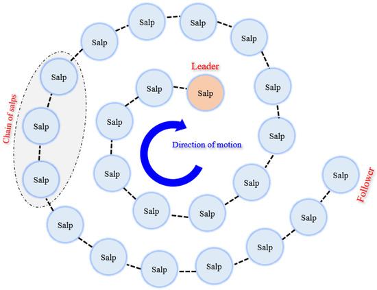
Figure 1.
The natural behavior of salp swam in the deep ocean.
(1) Updating of the leaders
Mathematical expression of the position updating strategy of the leader is given below:
where denotes the updating position of the leader in the dimension j in current iteration, wherein j = 1, 2, …, d and d is the number of decision variables; denotes the position of the food source in the dimension j of the previous generation, note that the position of the food source in the initial iteration is that of the individual salp with the best fitness value; and are the upper bound and lower bound of each salp in the dimension j, respectively. r1, r2, and r3 are the random numbers uniformly distributed in the interval [0, 1]. The functions of the three random numbers are different. The former is developed to find a balance between exploration and exploitation, whereas the latter two are used to control the salp walking in the positive direction or negative direction. Note that r1 decreases nonlinearly over the course of iterations, which can be expressed below:
where t denotes the current iteration; T denotes the maximum number of iterations.
(2) Updating of the followers
The inspiration of position updating of the followers comes from Newton’s law of motion, which can be expressed below:
where i = 1, 2, …, N, but here and N is the population size; denotes the updating position of the follower i in the dimension j in current iteration; a and w0 denote the acceleration and the velocity of the salp chain, respectively. It is noteworthy that the initial speed w0 is assumed to 0 and the discrepancy of time represented by iteration is set to 1. Thus, Equation (3) can be also expressed below:
The pseudo-code of the SSA can be found in the original paper [35].
3.2. Sine Cosine Operator
The sine cosine operator refers to the position updating strategy using sine and cosine functions in the SCA algorithm [35]. The sine and cosine operators are able to promote a search agent to update its position around another search agent. In other words, the SCA algorithm can control its ability of exploration and exploitation in the search space by adaptive adjustment of the range in the sine and cosine functions. The position updating equations using sine and cosine functions developed in the SCA algorithm can be expressed below:
where denotes the updating position of one search agent in dimension j at iteration t; c1, c2, c3 and c4 denotes random numbers; denotes the position of the best solution obtained so far in dimension j at iteration t. Note that denotes the absolute value between the current search agent and its reference one .
It is noteworthy that the random numbers c1, c2, c3, and c4 are applied to achieve different random functions. Among them, c1 is the most important parameter controlling the movement direction of one search agent to diverge from its reference or converge towards its reference to balance the exploration and exploitation of search agents, whereas c2 determines the step size of the movement towards or outwards the reference search agent; c3 is used to quantify the effect of the reference search agent on the distance between one search agent and its reference one; and c4 is applied to decide whether to use a sine function or a cosine function to perform position updating. Different from other parameters, c1 is updated over the course of iterations to balance exploration and exploitation, which can be expressed below:
where a is a constant.
3.3. Opposition-Based Learning
Opposition-based learning is a learning mechanism proposed by Tizhoosh [41]. The core idea of OBL is to help search agents enrich their search directions to generate neighboring solutions, thus approaching the global optimal solution faster. More concretely, OBL redirects each search agent in the opposite direction, which indirectly enriches the diversity of the population during optimization. From this point of view, OBL can promote the convergence rate of the algorithm by creating a new candidate search agent with the opposite direction of the current search agent to increase the selection pressure over the course of iterations. As a result, the convergence ability of the algorithm is improved, whereas the time consumption is decreased overall [41].
In summary, the OBL mechanism consists of two steps when applied in meta-heuristic algorithms. Firstly, the new search agent with the opposite position corresponding to the current search agent is generated, which can be expressed by Equation (20). Secondly, the fitness values of the new search agent and its corresponding one are evaluated and compared; then, the one with higher fitness value is selected to the next generation. The second step can be expressed by Equation (21):
where lb and ub are the lower and upper bounds of the search agent in current iteration t; , , and denote the search agent in the current search agent, the corresponding opposite search agent and the search agent selected to the next generation, respectively; and are the fitness values of , , respectively. Note that denotes that the performance of is better than or equal to that of and vice versa.
3.4. Elitism Strategy
Population is one of the important concepts in meta-heuristic algorithms. Population-based algorithms generate more than one search agent using a variety of stochastic generation mechanisms and improve them to expand the search space or enhance the local search ability over the course of iterations. A large number of studies have proved that a small population is prone to result in slow convergence rate and stagnation in local optima, whereas a large population can increase the probability of capturing the global optimal solution but suffer from huge computational costs and memory requirement [42]. To tackle this problem, population size that guarantees an optimal solution quickly enough has been a topic of intense research in past decades [43,44]. The compact GA (cGA) was proposed by Harik et al. [45] to generate offspring population by an estimation of distribution method instead of original recombination and mutation operators. It can provide a higher quality global optimal solution when solving simple optimization problems, while lacking the ability to solve the difficult optimization problems without exerting a higher selection pressure.
Elitism strategy effectively solves the above-mentioned problems. The best solution obtained so for is set as an elite solution and the worst solution in current iteration is replaced by an elite one to the next generation, preventing the loss of information of low salience. In other words, elitism strategy enhances the ability to find the best solution by increasing the selection pressure instead of increasing memory. As a result, elitism strategy has an effect on enriching the diversity of each population during optimization, leading to the improvement of the convergence rate and accuracy.
4. Proposed ISSA Algorithm
4.1. Proposed ISSA
As mentioned in the Introduction, SSA is simple yet effective to solve complex optimization problems, making it have extensive applications in various fields. Despite the merits of SSA, it can not solve all the optimization problems based on the No Free Lunch (NFL) theorem. In other words, SSA also faces some demerits. It has been found that SSA suffers from a slow convergence rate because of unbalanced exploration and exploitation and stagnation in local optima caused by poor exploration. To cope with such problems, multiple strategies are integrated to the original SSA to promote its convergence rate and the ability of balancing exploration and exploitation in this paper.
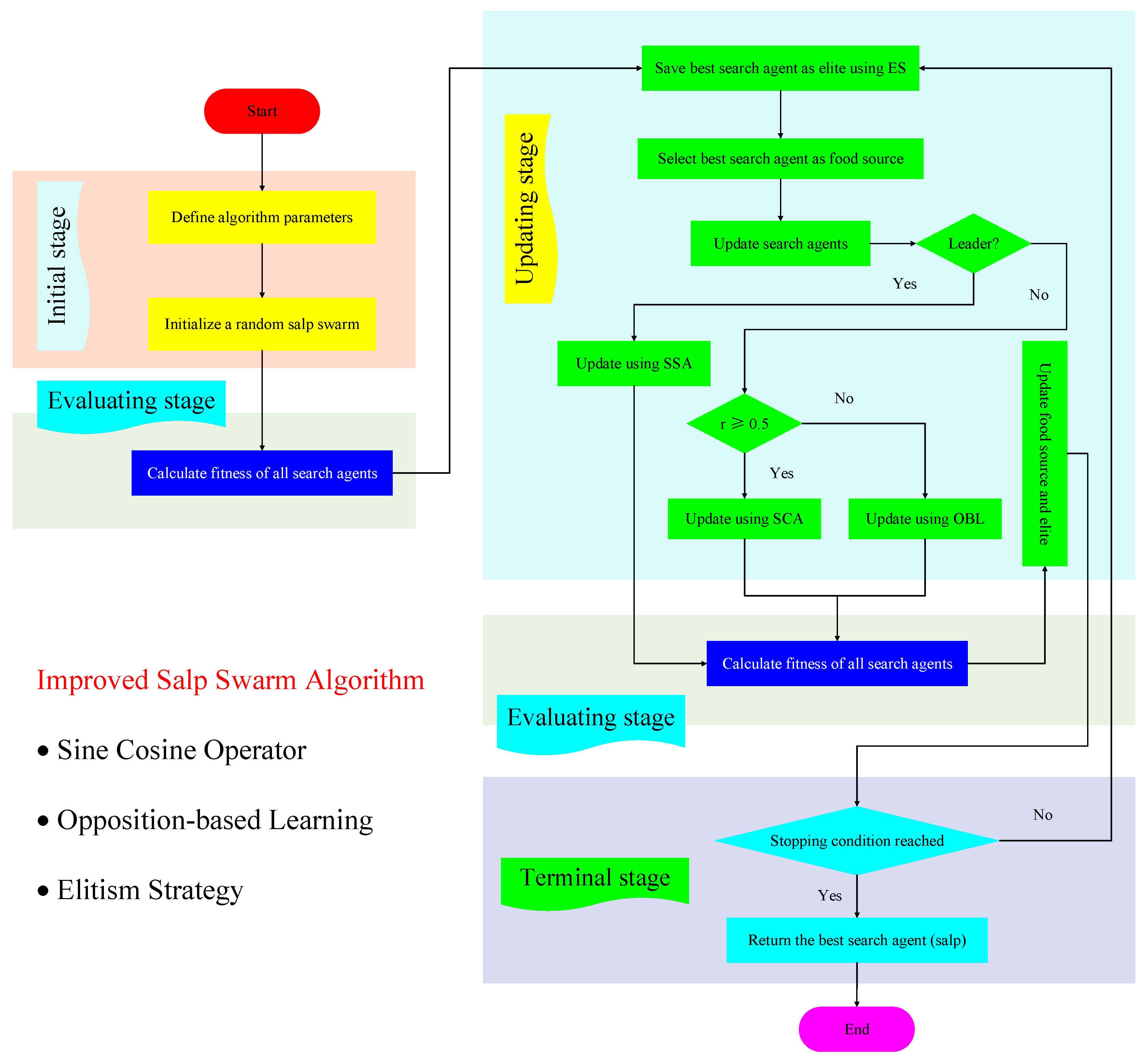
Needless to say, ISSA also consists of four steps similar to other population based meta-heuristic algorithms. Firstly, few algorithm parameters such as population size N, maximum number of iterations T, and number of decision variables d are defined and a random population (refer to salp swarm here) of solutions is generated in the initial stage. Secondly, the fitness value of each search agent (refer to a single salp here) is evaluated for leader selection in the evaluating stage. Thirdly, follower search agents are randomly updated by SCO and OBL. When a random number r is bigger than or equal to 0.5, the search agent is updated by SCO and vice versa. Then, one-to-one competition between the candidate search agent produced by SCO or OBL and the original search agent in the current iteration is conducted to obtain the better one. In addition, elitism strategy is applied to save the best search agent as elite in the current iteration in the updating stage. Fourthly, stopping condition is evaluated and the best search agent is obtained finally in the terminal stage. It is noteworthy that the third step is the core of the proposed ISSA, wherein population diversity is enriched to balance exploration and exploitation. For the sake of clarity, more detailed expression of ISSA is presented in Figure 2.
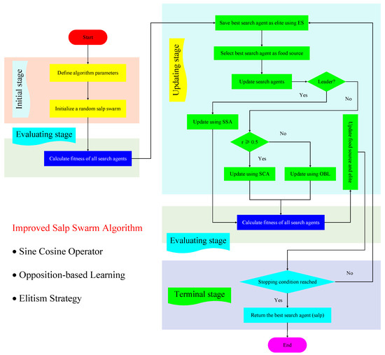
Figure 2.
Framework of the ISSA algorithm.
4.2. Computational Complexity
The goal of complexity analysis is to carry out quantitative analysis of time and space resources required by an algorithm during optimization. In this paper, the computational complexity with respect to ISSA can be determined by multiple strategies (SCO, OBL, and elitism) except original SSA itself, which can be expressed below:
where denotes Big O notation of computational complexity; Ns denotes the number of search agents handled by the SSA algorithm.
5. Experimental Evaluation and Discussion
5.1. Benchmark Functions
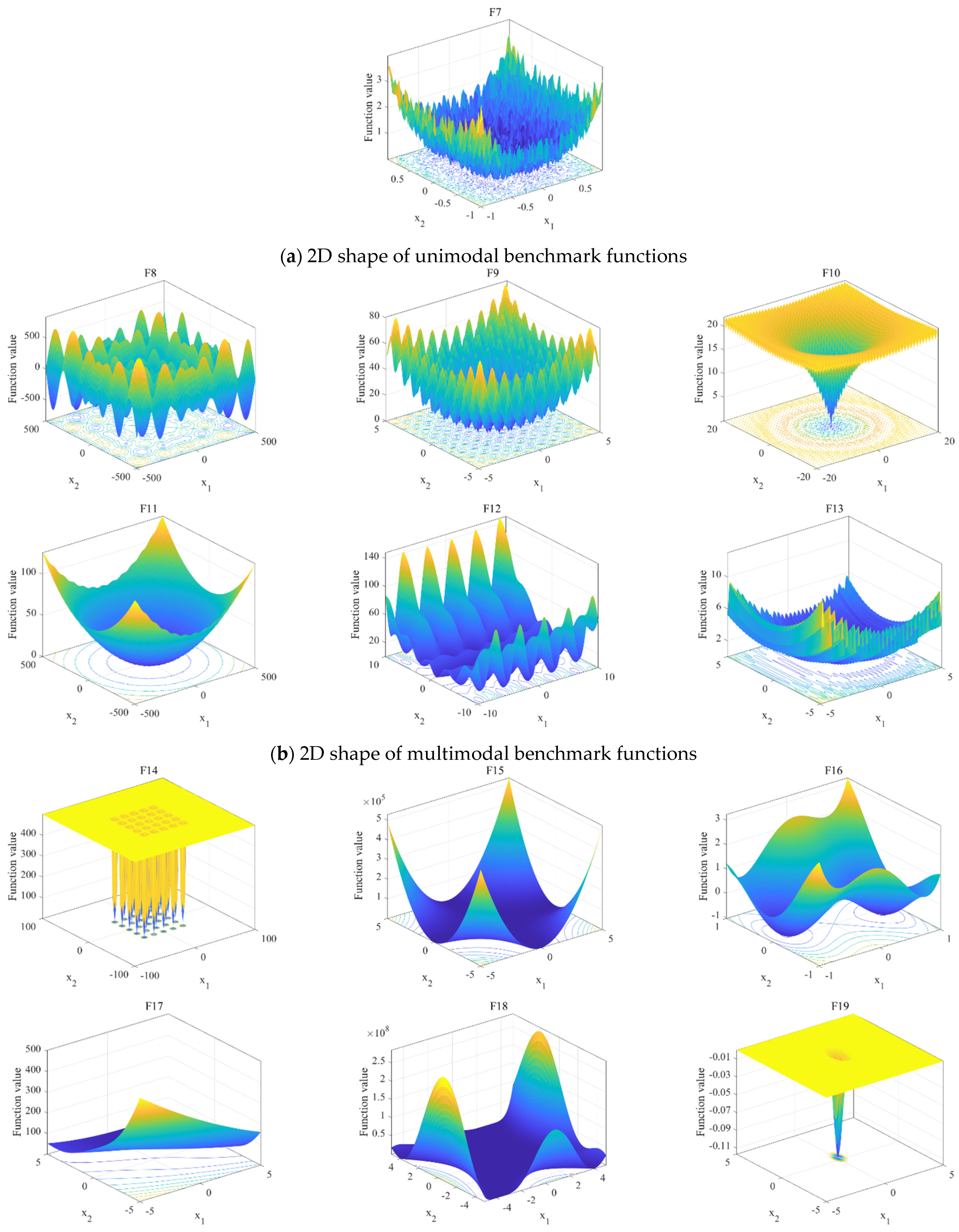
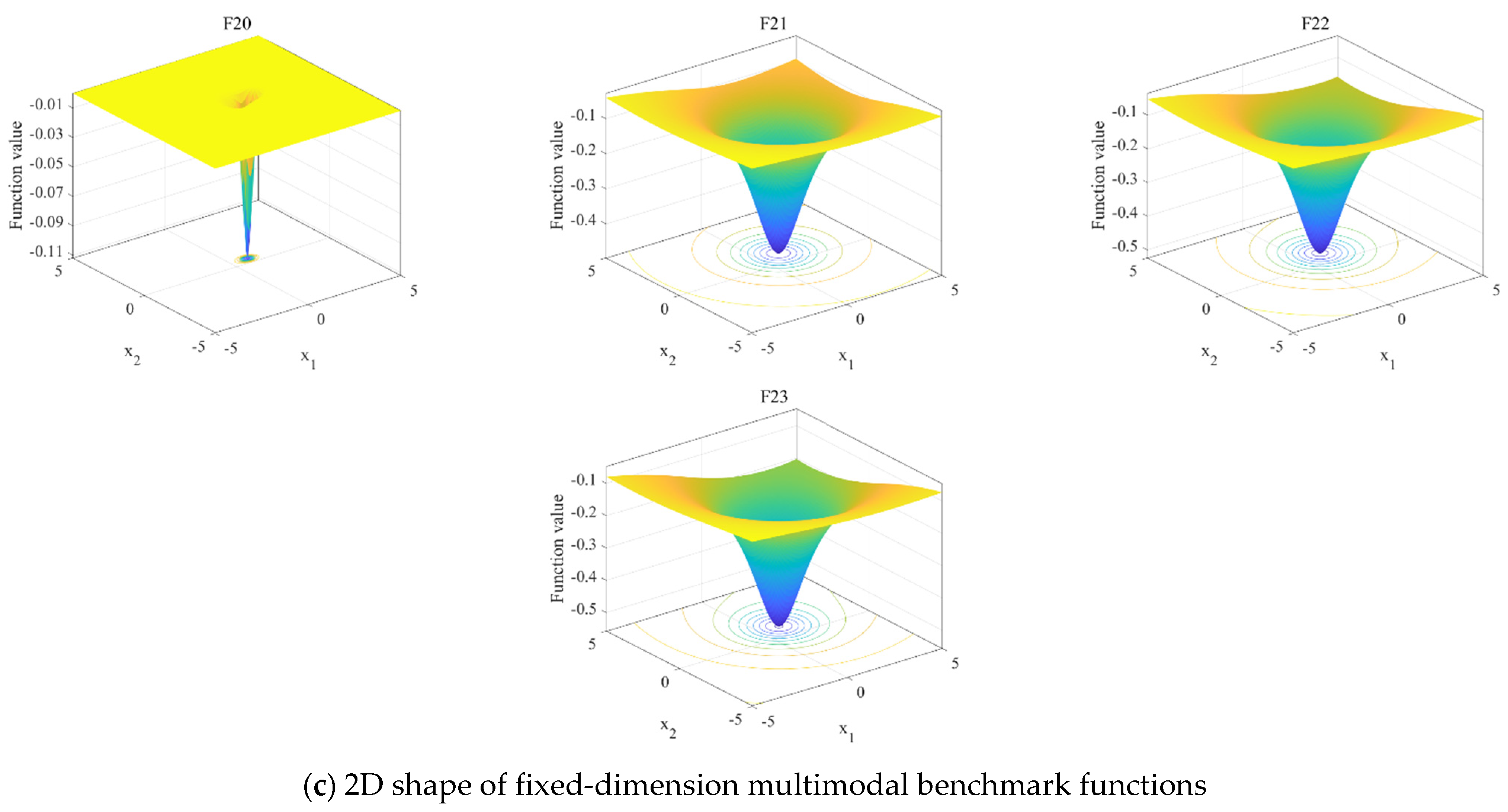
In this subsection, 23 classical benchmark functions with different characteristics widely used for meta-heuristics algorithms testing are adopted to testify the performance of ISSA. Such benchmark functions are widely applied to qualitative and quantitative analysis for meta-heuristic algorithms in a large number of studies in recent years [46,47,48], which can be divided into three types: unimodal (F1–F7), multimodal (F8–F13), and fixed-dimension multimodal (F14–F23). Note that all these benchmark functions are minimization problems.
The detailed descriptions of these benchmark functions are presented in Table 1, Table 2 and Table 3. The detailed information of the symbols in Table 1, Table 2 and Table 3 can be found in Mirjalili et al. [23]. In addition, their landscapes are illustrated in Figure 3. Figure 3 shows that unimodal benchmark functions only have one global optimal solution without any local minima. Thus, they can be used to test the performance of meta-heuristic algorithms on convergence rate. Additionally, Figure 3 shows that there are multiple local optimal solutions for multimodal benchmark functions, increasing the difficulty of searching the global optimal solution. Such benchmark functions are closer to the complex issues in real-world optimization. Therefore, they can be applied to benchmark the ability of meta-heuristic algorithms in terms of local optima avoidance and global search ability.

Table 1.
Unimodal benchmark functions.
Table 2.
Multimodal benchmark functions.
Table 3.
Fixed-dimension multimodal benchmark functions.
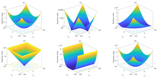

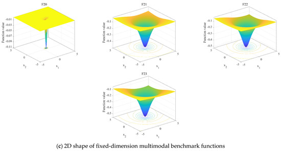
Figure 3.
Landscapes of benchmark functions.
5.2. Performance Comparison
In this subsection, the proposed ISSA is compared to the widely used meta-heuristic algorithm including PSO [32], GWO [23], WOA [33], SCA [35], MVO [49], and the original SSA. Average (Ave) and standard deviation (Std) are adopted as performance metrics to quantify the performance differences among such meta-heuristic algorithms, wherein Ave and Std are applied to verify how well and robust ISSA is while tackling optimization problems, respectively. Additionally, the boxplot method is employed to further verify the superiority of the proposed ISSA. For the sake of fair comparison, the number of search agents and maximum iteration are set to 50 and 1000, respectively. It is noteworthy that the parameter settings of other algorithms can refer to the source code in their corresponding original literature to maximize the performances. Each algorithm mentioned above run 30 times independently on benchmark functions. Then, the results including Ave and Std are obtained.
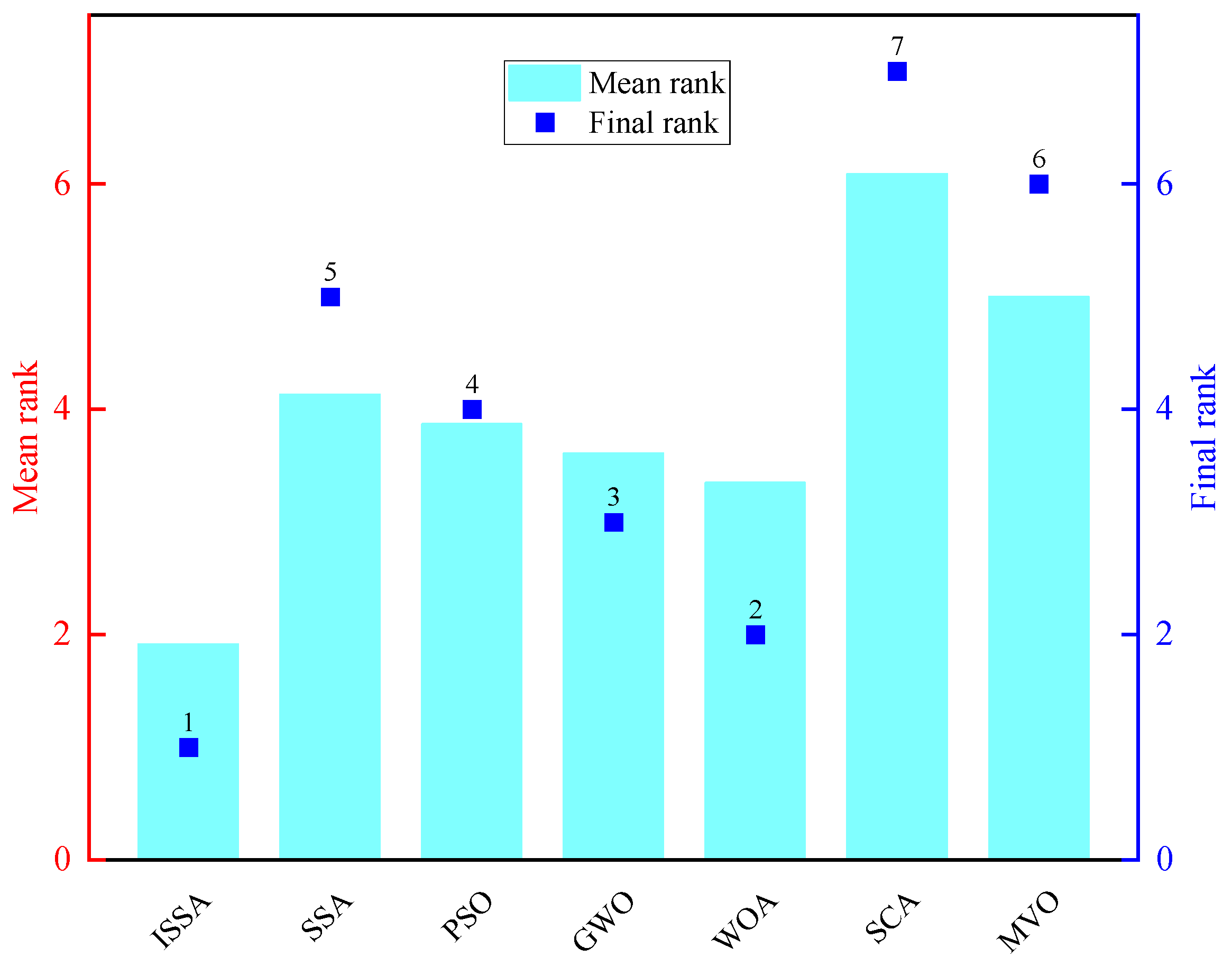
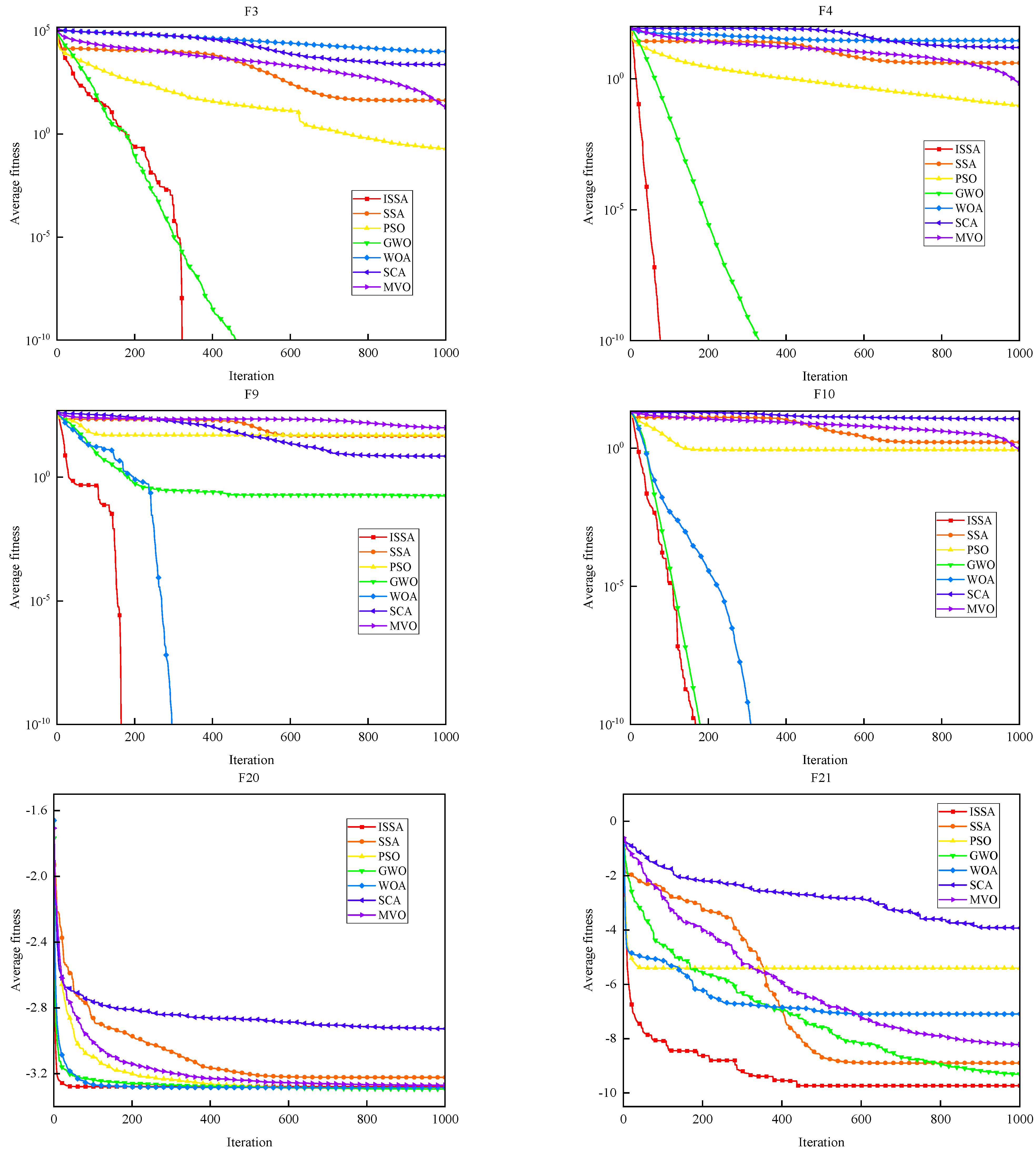
The statistic results in terms of Ave and Std of the best fitness values on each benchmark function were calculated by all algorithms mentioned above, as shown in Table 4, Table 5 and Table 6. Table 4, Table 5 and Table 6 show the statistic results on unimodal, multimodal, and fixed-dimension multimodal benchmark functions, respectively. F1–F7 are unimodal benchmark functions for benchmarking exploitation ability of meta-heuristic algorithms, whereas F8–F23 are multimodal ones for testing exploration ability of meta-heuristic algorithms. According to Table 4, ISSA performs better than all others in most of the benchmark functions including F1–F5 and F7. These results indicate that ISSA performs better in exploitation ability. In addition, Table 5 and Table 6 show that ISSA achieves the best candidate solutions for F8–F15 compared to all others, indicating that ISSA has good performance in terms of exploration ability. Figure 4 shows mean rank and final rank based on the statistic results. It can be observed from the mean rank that ISSA is ranked first and has the best overall performance, while WOA are the second best, followed by GWO, PSO, SSA, MVO, and SCA. Meanwhile, the ISSA algorithm is first with respect to final rank among all algorithms. Furthermore, in order to explore the convergence rate of the proposed algorithm, the convergence curves of all algorithms on several benchmark functions are given in Figure 5, wherein F3 and F4 represent unimodal functions, F9 and F10 represent multimodal functions, and F20 and F21 represent fixed-dimension functions. Figure 5 shows that ISSA has a faster convergence rate than all other algorithms, indicating its good convergence ability.
Table 4.
Statistical results of ISSA on unimodal benchmark functions.
Table 5.
Statistical results of ISSA on multimodal benchmark functions.
Table 6.
Statistical results of ISSA on fixed-dimension multimodal benchmark functions.

Figure 4.
Ranks of all algorithms based on the average values.
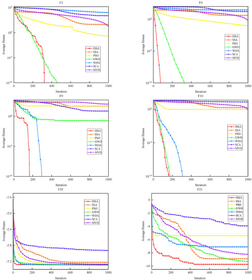
Figure 5.
Convergence curves of algorithms for selected six benchmark functions (F3, F4. F9, F10, F20, and F21).
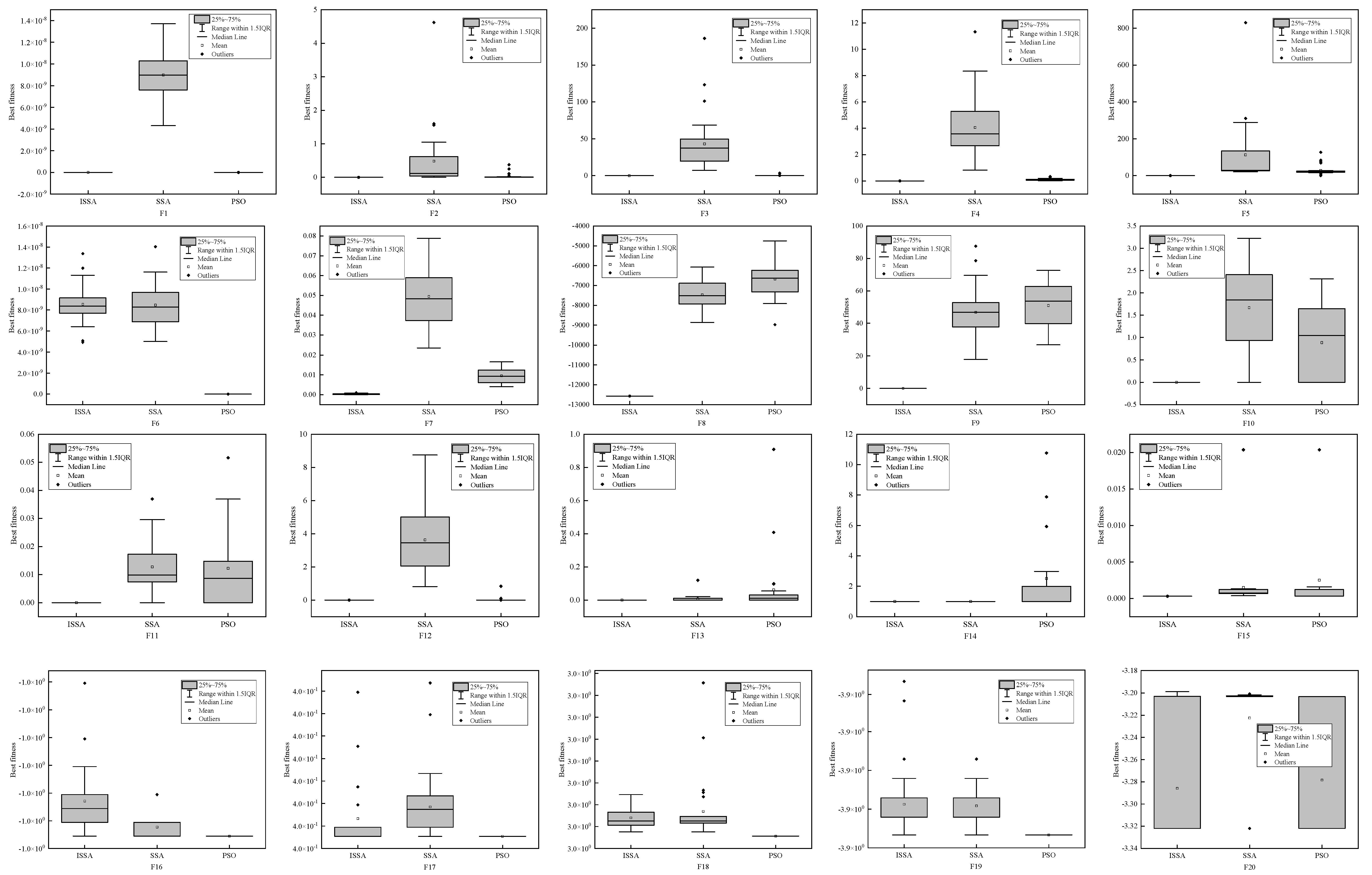
Furthermore, the boxplot is applied to graphically depict the distribution features of optimal solutions obtained by algorithms. Boxplot displays differences between populations without making any assumptions of the underlying statistical distribution and the spacings between the different parts of the box indicate the degree of dispersion (spread) and skewness in the data, and show outliers. The boxplots of ISSA, SSA, and PSO on 23 classical benchmark functions are shown in Figure 6. Figure 6 shows that ISSA has smaller best fitness values distribution and fewer outliers than most of other algorithms, indicating its stronger robustness and adaptability.
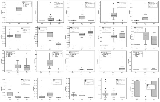
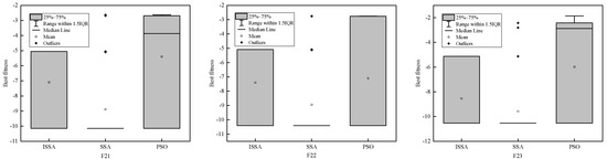
Figure 6.
Boxplot of several algorithms on 23 classical benchmark functions.
In summary, the ISSA algorithm is able to provide competitive performance on the 23 classical benchmark functions in contrast to other popular meta-heuristic algorithms. It substantially realizes the balance of exploration and exploitation, avoiding the drawback of original SSA easy to fall into local optimal solution, while having a faster convergence rate. This is mainly due to the multiple strategies introduced in this paper. SCO and OBL are able to promote the search agent to move toward the promising regions of the search space, while elitism strategy can avoid optimal search agent from being destroyed by position updating during optimization to promote the convergence rate. These results demonstrate that ISSA has advantages in exploration and exploitation.
5.3. Scalability Test for ISSA
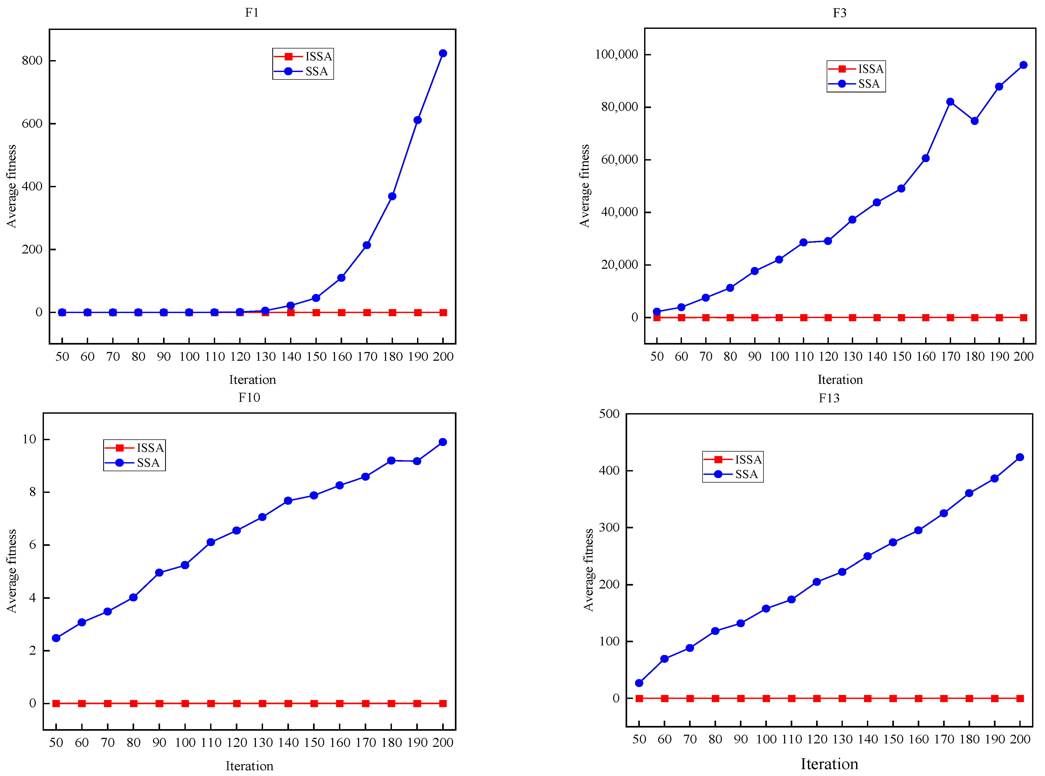
The optimization problems in the real world are much more complex than the benchmark problems mentioned above. Therefore, the property, also called scalability, of an algorithm to handle a growing amount of dimensions is important. In this subsection, the scalability test of ISSA compared to SSA is conducted to benchmark its performance with an increasing number of variables of benchmark functions. F1 and F3 are selected to represent unimodal benchmark functions. F10 and F13 are selected to represent multimodal benchmark functions. The number of dimension varies from 50 to 200 with the step size of 10 [35]. ISSA and SSA are run 30 times on the four benchmark functions at the same conditions, respectively, wherein the number of search agents is set to 50 and maximum iteration is set to 1000. The results of average best fitness values of 30 times run are given in Figure 7. Figure 7 shows that ISSA is able to find the optimal solution on F1, F3, F10, and F13, and its performance is stable with the increased dimensions. In addition, it can be observed that the performance of SSA on F1 does not significantly degrade when the dimension changes from 50 to 120. However, it gradually degrades with the dimension varying from 120 to 200. For F3, F10, and F13, it can be seen that the performance of SSA significantly degrades with the increased dimension from 50 to 200. In summary, the proposed ISSA has good scalability and the potential to solve optimization problems with high complexity in the real world.
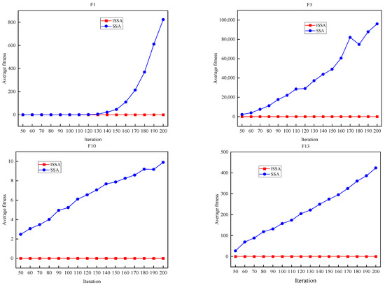
Figure 7.
Results of scalability test on four selected benchmark functions (F1, F3, F10, and F13) for ISSA.
6. Application to Optimal Operation of Multiple Reservoir Systems
6.1. Engineering Background
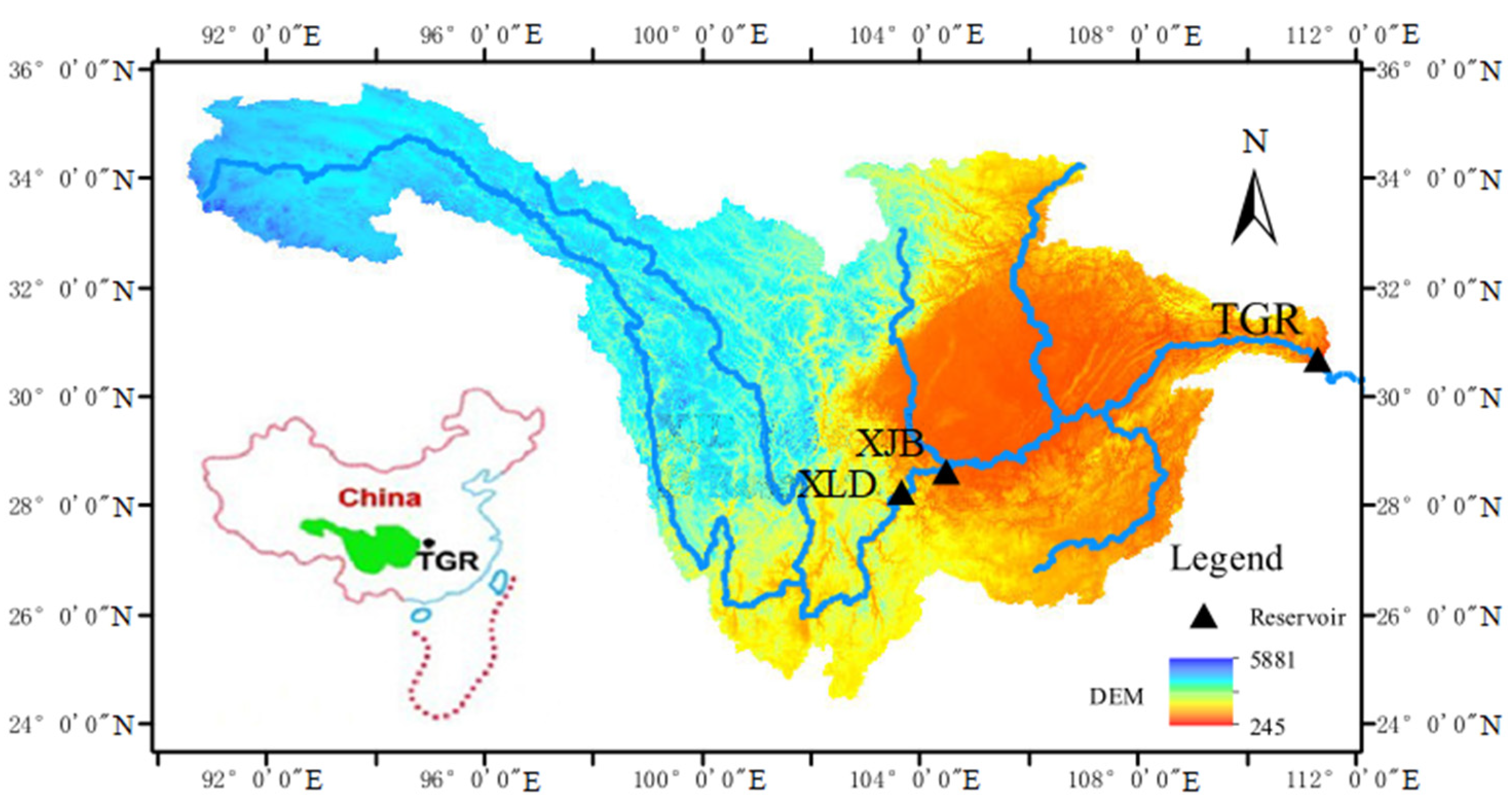
The Xiluodu Reservoir (XLD) and Xiangjiaba Reservoir (XJB) in the upper Yangtze River of China are selected as a case study. XLD and XJB are multiple hydropower reservoirs located in the lower reaches of Jinsha River. The location of XLD and XJB are shown in Figure 8. The designed installed capacities of XLD and XJB are 1260 × 104 kW and 600 × 104 kW, respectively, which are mainly for hydropower generation and have great comprehensive benefits in flood control, blocking, improving downstream shipping conditions, environmental, and social economy. It is noteworthy that there are two flood control tasks for XLD and XJB in flood season. Specifically, one is to ensure the flood control safety of downstream Sichuan-Chongqing reach, and the other is to cooperate with the Three Gorges Reservoir (TGR) for flood control in the middle and lower reaches of the Yangtze River on the premise of ensuring the safety of the dam itself. Therefore, the XLD and XJB multiple reservoir system is required to intercept a certain flood volume to reduce flood control pressure of TGR in the Jingjiang section and Chenglingji section in the middle and lower reaches of the Yangtze River. To guarantee the hydropower generation benefit in the case of specified intercepted flood volume, an effective and efficient optimization method needs to be developed for operators to make reasonable storage and release strategy for multiple hydropower reservoirs.
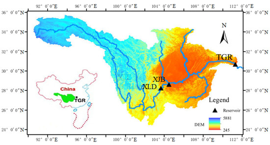
Figure 8.
Location of XLD and XJB cascade reservoirs.
6.2. Data
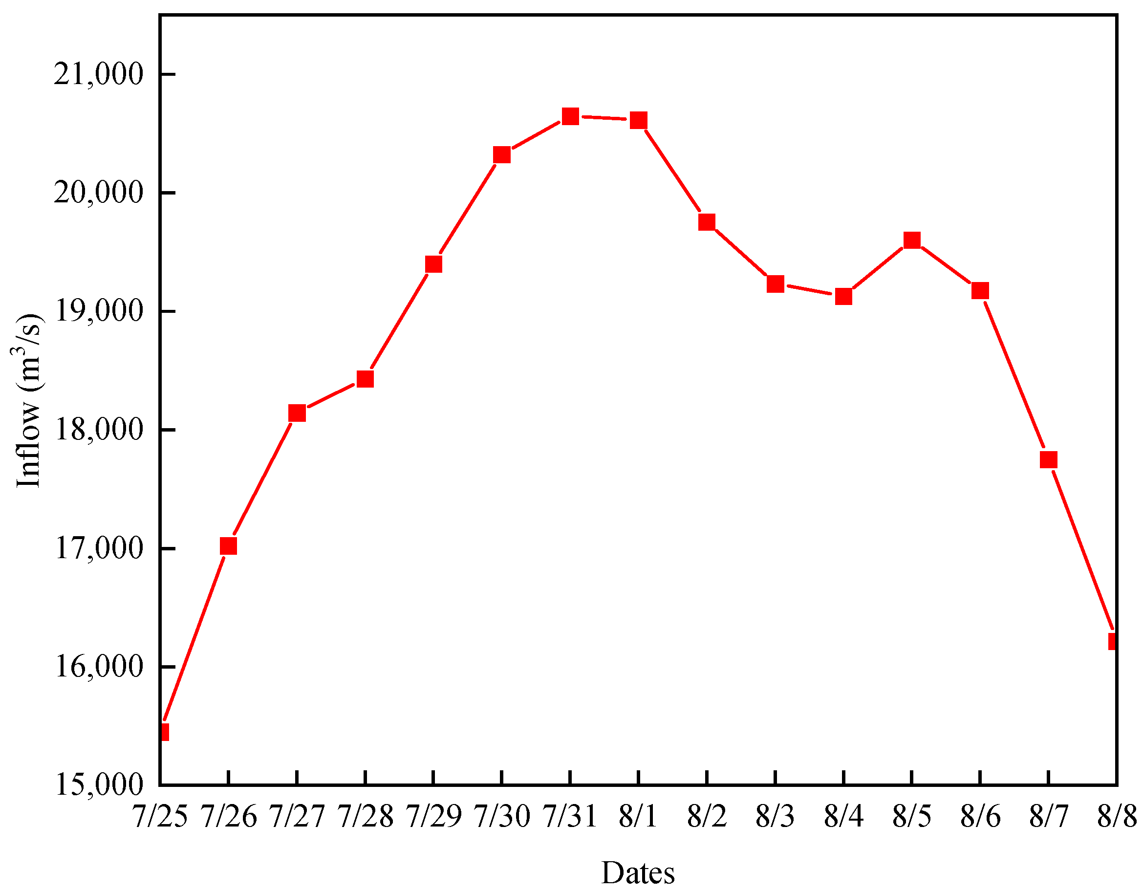
The typical flood with a 100 return period in 1954 from 1 June to 30 September is used as the original inflow. Then, the maximum 15-day flood hydrograph is obtained based on the original inflow and is from 25 July to 8 August, as shown in Figure 9. Figure 9 shows that the maximum 15-day flood hydrograph presents significant characteristics with double peak, increasing the difficulty of solving optimal operation of multiple hydropower reservoirs. The flood limiting water levels of XLD and XJB are 560 m and 370 m, respectively. The flood control water levels of XLD and XJB are 600 m and 380 m, respectively. The forebay water level fluctuations of XLD and XJB are 3 m and 4 m, respectively. Other parameters of the two reservoirs can be referred to their operation regulations.
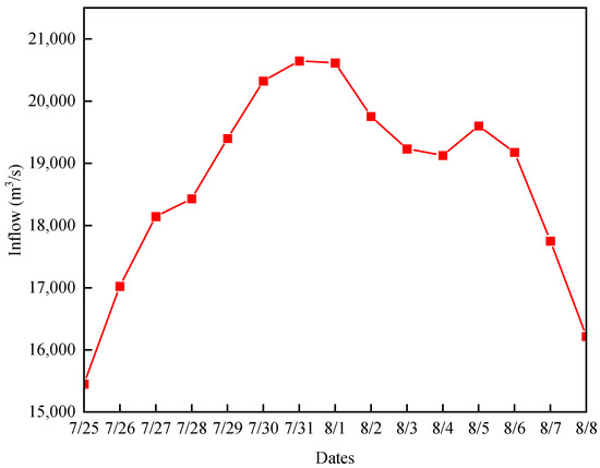
Figure 9.
Maximum 15-day flood hydrograph of typical flood with a 100 return period in 1954.
6.3. Results and Discussion
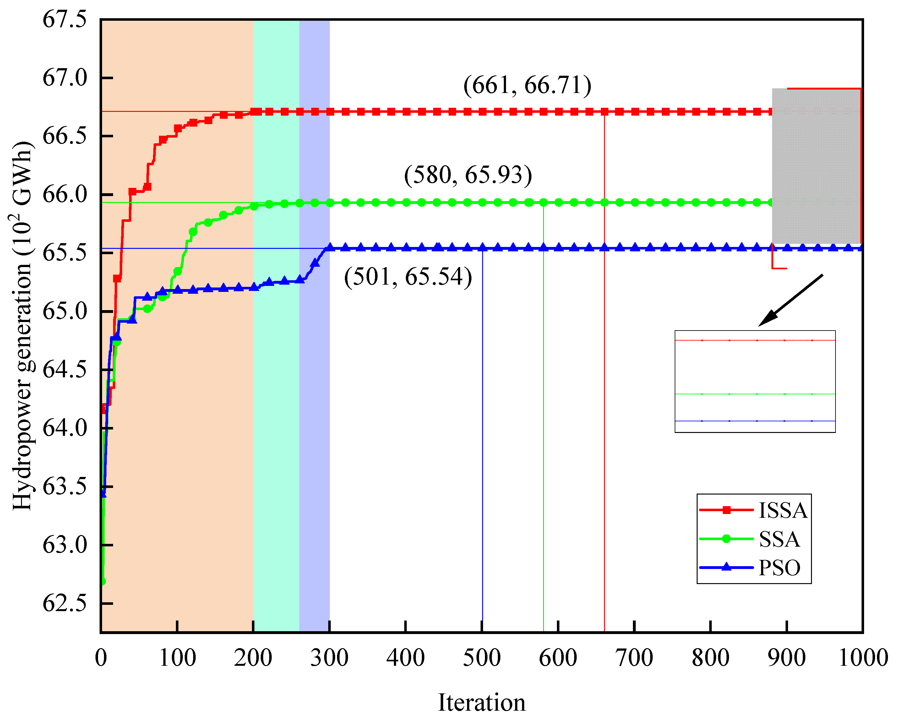
To verify the usefulness, ISSA is used for the optimal operation of XLD and XJB multiple hydropower reservoirs. The convergence curves of ISSA, SSA, and PSO algorithms for optimal operation are shown in Figure 10, indicating that the total hydropower generation of multiple reservoir system eventually converges to the optimal solution over the course of iterations. From the different background colors in Figure 10, the convergence rate of ISSA is higher than that of SSA, followed by PSO and the hydropower generation obtained by ISSA is bigger than that of SSA, followed by PSO. In addition, from the square view enlarged at the end of Figure 10, the optimal solutions by ISSA, SSA, and PSO are different, wherein the maximum hydropower generations obtained by ISSA, SSA, and PSO are 6671, 6593, and 6554 GWh, respectively. As a result, hydropower generation obtained by ISSA is increased by 1.18% compared to SSA and 1.77% compared to PSO, indicating the stronger exploration ability of ISSA for optimal operation of the multiple reservoir system.
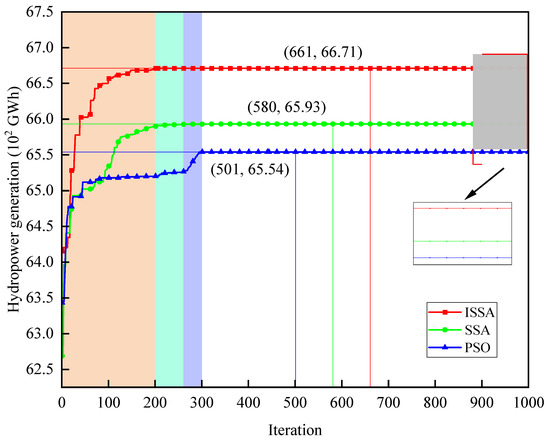
Figure 10.
Convergence curves of ISSA, SSA, and PSO for optimal operation.
In order to fully prove the effectiveness of the ISSA algorithm, water level, flow, and output processes are given in Figure 11, Figure 12 and Figure 13. Figure 11 shows that the water levels of XLD and XJB are all between their flood limiting water level and flood control water level. The absolute water level fluctuations of XLD and XJB are lower than 3 m and 4 m, respectively. This indicates the effectiveness of the constraints handling method. In addition, it can be observed that XLD operates at higher water levels by ISSA than SSA and PSO, while XJB operates at lower water levels by SSA and PSO. According to the regular operation scheme of the XLD and XJB multiple reservoir system in the flood season, the flood control capacity of XLD is first used in the operation sequence of reservoir capacity. When the water level of XLD rises to 573.1 m, the balance between the inflow and outflow of XLD is maintained, and XJB begins to intercept flood volume; when the flood control capacity of XJB is used up, XLD will continue to intercept. It can be seen from the operation results by ISSA in Figure 11 that the water level of XLD gradually increases from 560 m to 570 m from 25 July to 31 July, intercepting most of the flood volume in this stage. It can be seen from Table 7 that the optimized target water level of XLD and XJB by ISSA are 570.11 m and 376.58 m, respectively. The corresponding storage volume are 10.42 × 10⁸ m3 and 5.58 × 10⁸ m3, respectively, meeting the preset target storage volume 16 × 108 m3. This also indicates that XLD and XJB jointly intercept flood volume form the upper reaches of the Yangtze River. XLD and JXB undertake 65 % and 35 % of flood control task for the typical flood with 100 return period in 1954, respectively.
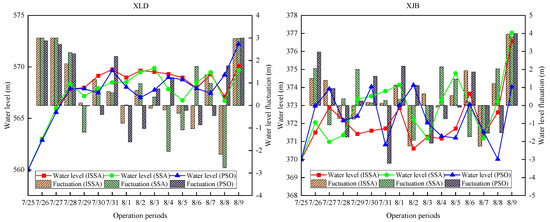
Figure 11.
Water level processes of XLD and XJB.
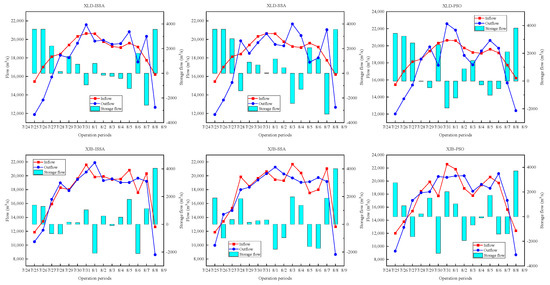
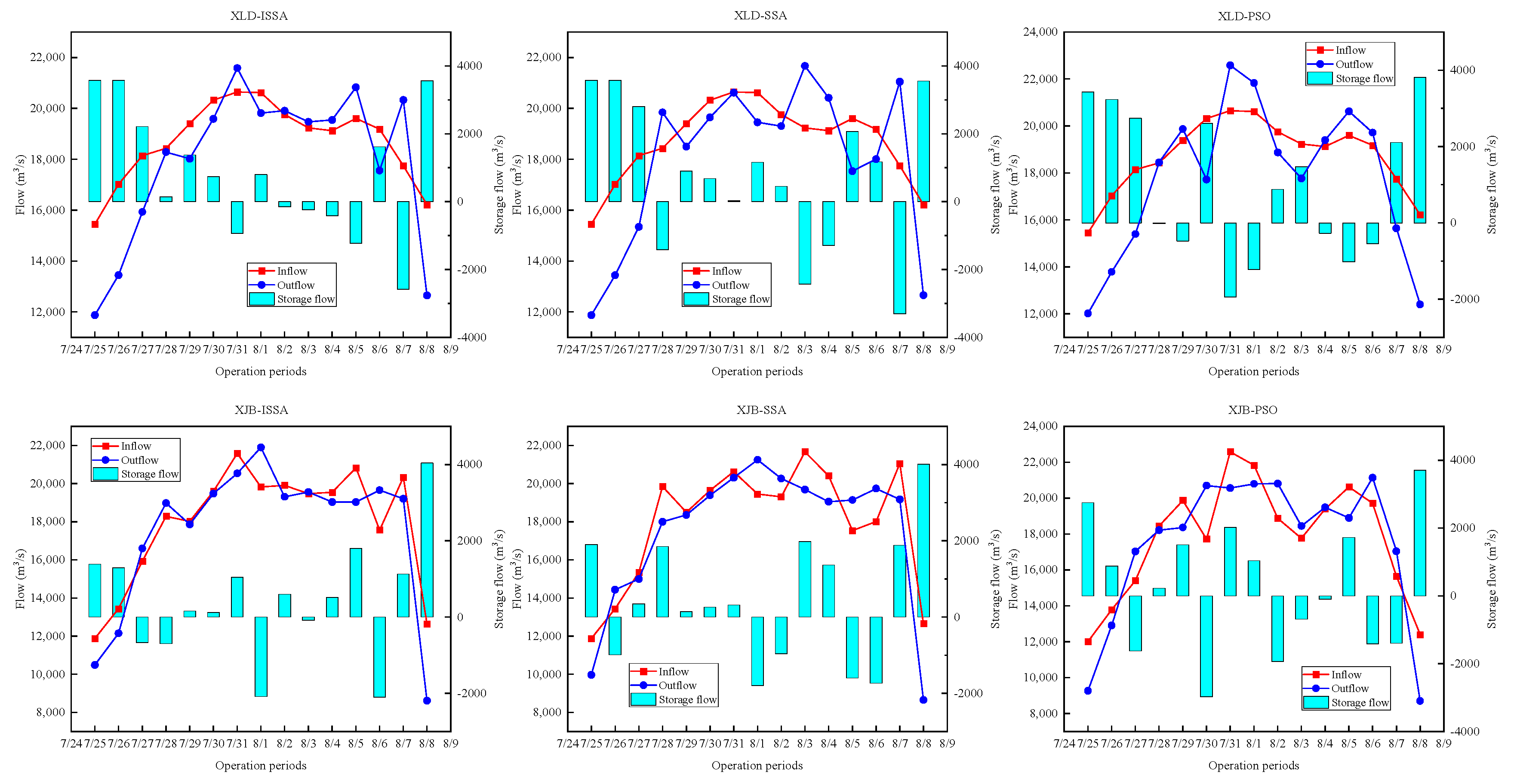
Figure 12.
Flow processes of XLD and XJB.
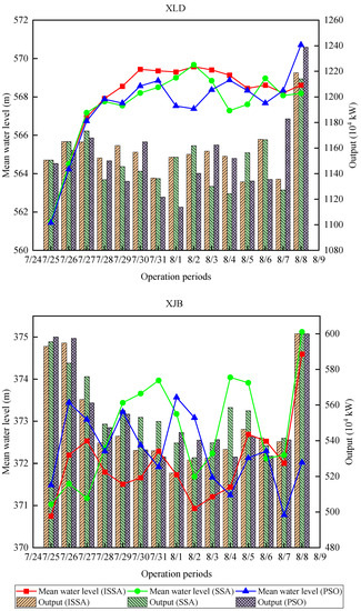
Figure 13.
Mean water level and output processes of XLD and XJB.
Table 7.
Storage volume of XLD and XJB cascade reservoirs.
It is noteworthy that XLD and XJB should make full use of flood resources while cooperating with TGR to intercept flood volume. Therefore, XLD then roughly maintains the balance of inflow and outflow and the corresponding absolute storage flow is low when its water level rises to 570 m (as shown in Figure 12), operating at a high water level. At the same time, the hydropower generation benefits of XLD are improved because of the high water head caused by high water level. It can be seen from Figure 12 that XJB cooperates with XLD and dynamically adjusts the storage and release capacity to meet the final flood control requirements, namely intercepting certain flood volume. However, the water levels and outflows of XLD and XJB obtained by SSA and PSO are different from those of ISSA. Firstly, the water levels of XLD obtained by SSA and PSO are lower than those of ISSA (as shown in Figure 11), reducing the hydropower generation benefits. Secondly, the water level and outflow fluctuations (as shown in Figure 11 and Figure 12) obtained by SSA and PSO are significantly larger than those of ISSA, which is not conducive to the safe and stable operation of cascade reservoirs.
Furthermore, the mean water level and output processes during optimization are given in Figure 12. It can be observed that the outputs of XLD and XJB all meet the power output limits, indicating the effectiveness of the constraints handling method. For XLD, the outputs calculated by ISSA are larger than those calculated by SSA and PSO, while XJB is on the contrary. This indicates that the contribution of XLD to the hydropower generation benefits for multiple hydropower reservoirs is greater than XJB. The reason is that XLD is first used to intercept flood volume while cooperating with TGR for the flood control of the middle and lower reaches of the Yangtze River and XLD operates at a higher water level by ISSA than SSA and PSO, resulting in the higher water head to produce more hydropower generation than SSA and PSO.
In summary, the optimal results including water level, outflow, and output by ISSA satisfy the complex constraints during optimal operation for multiple hydropower reservoirs. The second is that more hydropower generation can be obtained for multiple hydropower reservoirs by the proposed ISSA algorithm. Those demonstrate that ISSA can be used to solve complex optimal operation problem for multiple hydropower reservoirs.
7. Conclusions
In this study, a novel multiple strategy based salp swarm algorithm (ISSA) is proposed to cope with the drawbacks faced by the original SSA including slow convergence rate, unbalanced exploration and exploitation, and stagnation in local optima. Then, ISSA is used to the optimal operation of multiple hydropower reservoirs in the real world. The main contributions of this paper can be concluded below:
(1) Multiple strategies are integrated into SSA to enhance its performance. SCO is used to control balance between exploration and exploitation; the OBL is employed to promote the convergence rate of the algorithm, while the elitism strategy is adopted to enhance the ability to find the best solution by increasing the selection pressure.
(2) ISSA with multiple strategies is benchmarked by 23 classical benchmark functions. The results demonstrate that ISSA outperforms most of the well-known metaheuristic algorithms, and has good scalability and the potential to solve optimization problems with high complexity in the real world.
(3) ISSA is applied to optimal operation of XLD and XJB multiple reservoir systems in the upper Yangtze River. The results indicate that the proposed ISSA algorithm can solve the complex optimal operation problem effectively and efficiently. In addition, the maximum hydropower generation for XLD and XJB obtained by ISSA is 6671 GWh, increasing by 1.18% and 1.77% compared to SSA and PSO, respectively.
In the future, the feasibility of the ISSA algorithm in other complicated real-world engineering problems can be deepened.
Author Contributions
J.Z. conceived the original idea, and H.Q. designed the methodology. H.Q. and Y.Z. collected the data. H.Q. developed the code and performed the study. H.Q., J.Z., and L.C. contributed to the interpretation of the results. H.Q. wrote the paper, and J.Z. and L.C. revised the paper. All authors have read and agreed to the published version of the manuscript.
Funding
This research has been supported by the key project of the Natural Science Foundation of China (No. U1865202, No. 52039004), Natural Science Foundation of Hubei Province (No. 2020CFA101), Water conservancy science and technology innovation project of Guangdong province (No. 2020-23), National Natural Science Funds for Excellent Young Scholar (No. 51922047), State Key Laboratory of Simulation and Regulation of Water Cycle in River Basin of China (SKL2020ZY08).
Institutional Review Board Statement
Not applicable.
Informed Consent Statement
Not applicable.
Data Availability Statement
Due to the strict security requirements from the departments, some or all data, models, or code generated or used in the study are proprietary or confidential in nature and may only be provided with restrictions (e.g., anonymized data).
Acknowledgments
The authors also greatly appreciate the anonymous reviewers and academic editor for their careful comments and valuable suggestions to improve the manuscript. In addition, Hongya Qiu wants to thank, in particular, the invaluable support received from Bingyu Niu over the years.
Conflicts of Interest
The authors declare that no conflict of interest.
References
- Labadie, J.W. Optimal operation of multireservoir systems: State-of-the-art review. J. Water Resour. Plan. Manag. 2004, 130, 93–111. [Google Scholar] [CrossRef]
- Ren, K.; Huang, S.; Huang, Q.; Wang, H.; Leng, G.; Wu, Y. Defining the robust operating rule for multi-purpose water reservoirs under deep uncertainties. J. Hydrol. 2019, 578, 124134. [Google Scholar] [CrossRef]
- Feng, Z.K.; Liu, S.; Niu, W.J.; Li, S.S.; Wu, H.J.; Wang, J.Y. Ecological operation of cascade hydropower reservoirs by elite-guide gravitational search algorithm with Lévy flight local search and mutation. J. Hydrol. 2020, 581, 124425. [Google Scholar] [CrossRef]
- Niu, W.J.; Feng, Z.K.; Liu, S.; Chen, Y.B.; Xu, Y.S.; Zhang, J. Multiple hydropower reservoirs operation by hyperbolic grey wolf optimizer based on elitism selection and adaptive mutation. Water Resour. Manag. 2021, 35, 573–591. [Google Scholar] [CrossRef]
- Herman, J.D.; Quinn, J.D.; Steinschneider, S.; Giuliani, M.; Fletcher, S. Climate adaptation as a control problem: Review and perspectives on dynamic water resources planning under uncertainty. Water Resour. Res. 2020, 56, e24389. [Google Scholar] [CrossRef]
- SeethaRam, K.V. Three level rule curve for optimum operation of a multipurpose reservoir using genetic algorithms. Water Resour. Manag. 2021, 35, 353–368. [Google Scholar] [CrossRef]
- Deveci, K.; Güler, Ö. A CMOPSO based multi-objective optimization of renewable energy planning: Case of Turkey. Renew. Energy 2020, 155, 578–590. [Google Scholar] [CrossRef]
- Yu, L.; Li, Y.P.; Huang, G.H. A fuzzy-stochastic simulation-optimization model for planning electric power systems with considering peak-electricity demand: A case study of Qingdao, China. Energy 2016, 98, 190–203. [Google Scholar] [CrossRef]
- Lv, S.; He, W.; Zhang, A.; Li, G.; Luo, B.; Liu, X. Modelling and analysis of a novel compressed air energy storage system for trigeneration based on electrical energy peak load shifting. Energy Convers. Manag. 2017, 135, 394–401. [Google Scholar] [CrossRef]
- Yue, Q.; Guo, P. Managing agricultural water-energy-food-environment nexus considering water footprint and carbon footprint under uncertainty. Agric. Water Manag. 2021, 252, 106899. [Google Scholar] [CrossRef]
- Pfister, S.; Scherer, L.; Buxmann, K. Water scarcity footprint of hydropower based on a seasonal approach-Global assessment with sensitivities of model assumptions tested on specific cases. Sci. Total Environ. 2020, 724, 138188. [Google Scholar] [CrossRef]
- Qiu, H.; Chen, L.; Zhou, J.; He, Z.; Zhang, H. Risk analysis of water supply-hydropower generation-environment nexus in the cascade reservoir operation. J. Clean. Prod. 2021, 283, 124239. [Google Scholar] [CrossRef]
- Dai, Q.; Zhu, X.; Zhuo, L.; Han, D.; Liu, Z.; Zhang, S. A hazard-human coupled model (HazardCM) to assess city dynamic exposure to rainfall-triggered natural hazards. Environ. Model. Softw. 2020, 127, 104684. [Google Scholar] [CrossRef]
- Sansare, D.A.; Mhaske, S.Y. Natural hazard assessment and mapping using remote sensing and QGIS tools for Mumbai city, India. Nat. Hazards 2020, 100, 1117–1136. [Google Scholar] [CrossRef]
- Zhu, F.; Zhong, P.A.; Xu, B.; Wu, Y.N.; Zhang, Y. A multi-criteria decision-making model dealing with correlation among criteria for reservoir flood control operation. J. Hydroinformatics 2016, 18, 531–543. [Google Scholar] [CrossRef]
- Feng, Z.K.; Liu, S.; Niu, W.J.; Li, B.J.; Wang, W.C.; Luo, B.; Miao, S.M. A modified sine cosine algorithm for accurate global optimization of numerical functions and multiple hydropower reservoirs operation. Knowl.-Based Syst. 2020, 208, 106461. [Google Scholar] [CrossRef]
- Pan, Z.; Chen, L.; Teng, X. Research on joint flood control operation rule of parallel reservoir group based on aggregation–decomposition method. J. Hydrol. 2020, 590, 125479. [Google Scholar] [CrossRef]
- Wang, X.; Hu, T.; Zeng, X.; Zhang, Q.; Huang, J. A bilevel modeling framework to analyze the institutional gap between research and operation practices–Case on the Three Gorges Reservoir pre-impoundment problem. J. Hydrol. 2020, 585, 124742. [Google Scholar] [CrossRef]
- Chang, J.; Meng, X.; Wang, Z.; Wang, X.; Huang, Q. Optimized cascade reservoir operation considering ice flood control and power generation. J. Hydrol. 2014, 519, 1042–1051. [Google Scholar] [CrossRef]
- He, W.; Ma, C.; Zhang, J.; Lian, J.; Wang, S.; Zhao, W. Multi-objective optimal operation of a large deep reservoir during storage period considering the outflow-temperature demand based on NSGA-II. J. Hydrol. 2020, 586, 124919. [Google Scholar] [CrossRef]
- Liu, X.; Chen, L.; Zhu, Y.; Singh, V.P.; Qu, G.; Guo, X. Multi-objective reservoir operation during flood season considering spillway optimization. J. Hydrol. 2017, 552, 554–563. [Google Scholar] [CrossRef]
- Ferdowsi, A.; Singh, V.P.; Ehteram, M.; Mirjalili, S. Multi-objective Optimization Approaches for Design, Planning, and Management of Water Resource Systems. In Essential Tools for Water Resources Analysis, Planning, and Management; Springer: Singapore, 2021; pp. 275–303. [Google Scholar]
- Mirjalili, S.; Mirjalili, S.M.; Lewis, A. Grey wolf optimizer. Adv. Eng. Softw. 2014, 69, 46–61. [Google Scholar] [CrossRef] [Green Version]
- Zhou, Y.; Guo, S.; Chang, F.J.; Liu, P.; Chen, A.B. Methodology that improves water utilization and hydropower generation without increasing flood risk in mega cascade reservoirs. Energy 2018, 143, 785–796. [Google Scholar] [CrossRef]
- Rahimi, H.; Ardakani, M.K.; Ahmadian, M.; Tang, X. Multi-Reservoir Utilization Planning to Optimize Hydropower Energy and Flood Control Simultaneously. Environ. Process. 2020, 7, 41–52. [Google Scholar] [CrossRef]
- Feng, Z.K.; Niu, W.J.; Zhang, R.; Wang, S.; Cheng, C.T. Operation rule derivation of hydropower reservoir by k-means clustering method and extreme learning machine based on particle swarm optimization. J. Hydrol. 2019, 576, 229–238. [Google Scholar] [CrossRef]
- Yang, S.; Yang, D.; Chen, J.; Zhao, B. Real-time reservoir operation using recurrent neural networks and inflow forecast from a distributed hydrological model. J. Hydrol. 2019, 579, 124229. [Google Scholar] [CrossRef]
- Suwal, N.; Huang, X.; Kuriqi, A.; Chen, Y.; Pandey, K.P.; Bhattarai, K.P. Optimisation of cascade reservoir operation considering environmental flows for different environmental management classes. Renew. Energy 2020, 158, 453–464. [Google Scholar] [CrossRef]
- Hayyolalam, V.; Kazem, A.A.P. Black widow optimization algorithm: A novel meta-heuristic approach for solving engineering optimization problems. Eng. Appl. Artif. Intell. 2020, 87, 103249. [Google Scholar] [CrossRef]
- Back, T. Evolutionary Algorithms in Theory and Practice: Evolution Strategies, Evolutionary Programming, Genetic Algorithms; Oxford University Press: Oxford, England, 1996. [Google Scholar]
- Blum, C.; Li, X. Swarm Intelligence in Optimization. In Swarm Intelligence; Springer: Berlin/Heidelberg, Germany, 2008; pp. 43–85. [Google Scholar]
- Eberhart, R.; Kennedy, J. A new optimizer using particle swarm theory. In Proceedings of the Sixth International Symposium on Micro Machine and Human Science, Nagoya, Japan, 4–6 October 1995; pp. 39–43. [Google Scholar]
- Mirjalili, S.; Lewis, A. The whale optimization algorithm. Adv. Eng. Softw. 2016, 95, 51–67. [Google Scholar] [CrossRef]
- Karaboga, D.; Basturk, B. A powerful and efficient algorithm for numerical function optimization: Artificial bee colony (ABC) algorithm. J. Glob. Optim. 2007, 39, 459–471. [Google Scholar] [CrossRef]
- Mirjalili, S. SCA: A sine cosine algorithm for solving optimization problems. Knowl.-Based Syst. 2016, 96, 120–133. [Google Scholar] [CrossRef]
- Mirjalili, S.; Gandomi, A.H.; Mirjalili, S.Z.; Saremi, S.; Faris, H.; Mirjalili, S.M. Salp Swarm Algorithm: A bio-inspired optimizer for engineering design problems. Adv. Eng. Softw. 2017, 114, 163–191. [Google Scholar] [CrossRef]
- Wolpert, D.H.; Macready, W.G. No free lunch theorems for optimization. IEEE Trans. Evol. Comput. 1997, 1, 67–82. [Google Scholar] [CrossRef] [Green Version]
- Rahnamayan, S.; Tizhoosh, H.R.; Salama, M.M. Opposition-based differential evolution. IEEE Trans. Evol. Comput. 2008, 12, 64–79. [Google Scholar] [CrossRef] [Green Version]
- Feng, Z.K.; Niu, W.J.; Cheng, X.; Wang, J.Y.; Wang, S.; Song, Z.G. An effective three-stage hybrid optimization method for source-network-load power generation of cascade hydropower reservoirs serving multiple interconnected power grids. J. Clean. Prod. 2020, 246, 119035. [Google Scholar] [CrossRef]
- Bone, Q.; Trueman, E.R. Jet propulsion in salps (Tunicata: Thaliacea). J. Zool. 1983, 201, 481–506. [Google Scholar] [CrossRef]
- Tizhoosh, H.R. Opposition-based learning: A new scheme for machine intelligence. In Proceedings of the International Conference on Computational Intelligence for Modelling, Control and Automation and International Conference on Intelligent Agents, Web Technologies and Internet Commerce (CIMCA-IAWTIC’06), Vienna, Austria, 28–30 November 2005; Volume 1, pp. 695–701. [Google Scholar]
- Ahn, C.W.; Ramakrishna, R.S. Elitism-based compact genetic algorithms. IEEE Trans. Evol. Comput. 2003, 7, 367–385. [Google Scholar]
- Reed, P.M.; Hadka, D.; Herman, J.D.; Kasprzyk, J.R.; Kollat, J.B. Evolutionary multiobjective optimization in water resources: The past, present, and future. Adv. Water Resour. 2013, 51, 438–456. [Google Scholar] [CrossRef] [Green Version]
- Mansouri, N.; Javidi, M.M. A review of data replication based on meta-heuristics approach in cloud computing and data grid. Soft Comput. 2020, 1–28. [Google Scholar] [CrossRef]
- Harik, G.R.; Lobo, F.G.; Goldberg, D.E. The compact genetic algorithm. IEEE Trans. Evol. Comput. 1999, 3, 287–297. [Google Scholar] [CrossRef] [Green Version]
- Yao, X.; Liu, Y.; Lin, G. Evolutionary programming made faster. IEEE Trans. Evol. Comput. 1999, 3, 82–102. [Google Scholar]
- Xu, Y.; Chen, H.; Heidari, A.A.; Luo, J.; Zhang, Q.; Zhao, X.; Li, C. An efficient chaotic mutative moth-flame-inspired optimizer for global optimization tasks. Expert Syst. Appl. 2019, 129, 135–155. [Google Scholar] [CrossRef]
- Muthusamy, H.; Ravindran, S.; Yaacob, S.; Polat, K. An improved elephant herding optimization using sine–cosine mechanism and opposition based learning for global optimization problems. Expert Syst. Appl. 2021, 172, 114607. [Google Scholar] [CrossRef]
- Mirjalili, S.; Mirjalili, S.M.; Hatamlou, A. Multi-verse optimizer: A nature-inspired algorithm for global optimization. Neural Comput. Appl. 2016, 27, 495–513. [Google Scholar] [CrossRef]


Publisher’s Note: MDPI stays neutral with regard to jurisdictional claims in published maps and institutional affiliations. |
© 2021 by the authors. Licensee MDPI, Basel, Switzerland. This article is an open access article distributed under the terms and conditions of the Creative Commons Attribution (CC BY) license (https://creativecommons.org/licenses/by/4.0/).