Deep Learning Based Filtering Algorithm for Noise Removal in Underwater Images

Abstract

Under-water sensing and image processing play major roles in oceanic scientific studies. One of the related challenges is that the absorption and scattering of light in underwater settings degrades the quality of the imaging. The major drawbacks of underwater imaging are color distortion, low contrast, and loss of detail (especially edge information). The paper proposes a method to address these issues by de-noising and increasing the resolution of the image using a model network trained on similar data. The network extracts frames from a video and filters them with a trigonometric–Gaussian filter to eliminate the noise in the image. It then applies contrast limited adaptive histogram equalization (CLAHE) to improvise the image contrast, and finally enhances the image resolution. Experimental results show that the proposed method could effectively produce enhanced images from degraded underwater images.

1. Introduction

As with light propagating through the air, underwater light propagation is affected by scattering and absorption. Nonetheless, absorption and scattering have enormous magnitudes. While light attenuation coefficients in the air are measured in inverse kilometers, they are measured in inverse meters in an underwater environment [1]. Such severe light degradation creates significant challenges for imaging sensors attempting to acquire information about the underwater area of interest. Unlike air, water is transparent to the visible spectrum but opaque to all other wavelengths. The visible spectrum’s constituent wavelengths absorb at varying rates, with longer wavelengths absorbing more rapidly. Light energy decays in water in truly remarkable ways. By the time light energy reaches a depth of 150 m in the crystal-clear waters of the middle oceans, less than 1% of light energy remains. Thus, in oceans, the visibility is reduced beyond 20 m and in turbid coastal water the visibility is reduced beyond 5 m. Additionally, no natural light from the sun reaches below 1 km from the sea. As a result, the amount of light contained within water is always less than the amount of light above the water’s surface. This leads to the poor visual quality of the underwater images [2]. Underwater, light is typically scarce due to two unavoidable facts. One, light loses its true intensity when it is submerged, and two, the likelihood of light scattering within water is quite high. This insufficient amount of light has an immediate effect on the colour distortion and illumination of the underwater scene’s visibility. The absorption of light energy and the random path change of light beams as they travel through a water medium filled with suspended particles are two of the most detrimental effects on underwater image quality. The portion of light energy that enters the water is rapidly absorbed and converted to other forms of energy, such as heat, which energizes and warms the water molecules, causing them to evaporate. Additionally, some of the light energy is consumed by the microscopic plant-based organisms that utilize it for photosynthesis. This absorption reduces the underwater objects’ true colour intensity. As previously stated, some light that is not absorbed by water molecules may not travel in a straight line but rather follows a random Brownian motion. This is due to the presence of suspended matter in water. Water, particularly seawater, contains dissolved salts and organic and inorganic matter that reflects and deflects the light beam in new directions and may also float to the surface of the water and decay back into the air [3]. The scattering of light in a liquid medium is further classified into two types. Forward scattering refers to the deflection of the light beam after it strikes the object of interest and reaches the image sensor. Typically, this type of scattering causes an image to appear blurry. The other type of scattering is backscattering, which occurs when the light beam strikes the image sensor without being reflected by the object. In some ways, this is the light energy that contains no information about the object. It merely contributes to an image’s degraded contrast.

One way to improve visibility underwater is to introduce an artificial light source, though this solution introduces its own complications [4]. Apart from the issues mentioned previously, such as light scattering and attenuation, artificial light tends to illuminate the scene of interest in a non-uniform manner, resulting in a bright spotting in the image’s center and darker shades surrounding it. As lighting equipment is cumbersome and expensive, they may require a constant supply of electricity, either from batteries or a surface ship.

As a result, the underwater imaging system is no longer only affected by low light conditions, severely reduced visibility, diminishing contrast, burliness, and light artefacts, but also by colour range and random noise limitations. As a result, the standard image processing techniques that we rely on for terrestrial image enhancement must be modified or abandoned entirely, and new solutions must be developed. Significantly, increasing the quality of underwater images can result in improved image segmentation, feature extraction, and underwater navigation algorithms for self-driving underwater vehicles. Additionally, offshore drilling platforms may benefit from improved imagery for assessing the structural strength of their rigs’ underwater sections.

The absorption of light energy and the dispersion in the media contribute to the scattering effect which may be forward or backward scattering as shown in Figure 1. The forward scattering of light (also known as random dispersion) is higher in water than in air and that also results in further blurring of the images. Backward scattering is the fraction of light that is reflected back to the camera by water molecules before it hits the object of interest [5]. Back scattering gives a hazed appearance to the captured image due to the superimposition of reflections.

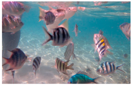
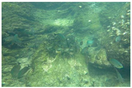
The images which are considered for analysis in this paper are underwater images. Absorption and scattering are further catalyzed by other elements such as small floating particles or dissolved organic matter. The floating particles present recognized as “marine snow” (highly variable both in nature and concentration) is one common factor that increases the effects of absorption and scattering. Artificial lighting used in underwater imaging is another cause for blurring due to scatter and absorption. Artificial lighting from point sources also causes non-uniform lighting on the image, often giving a brighter center compared to the edges.

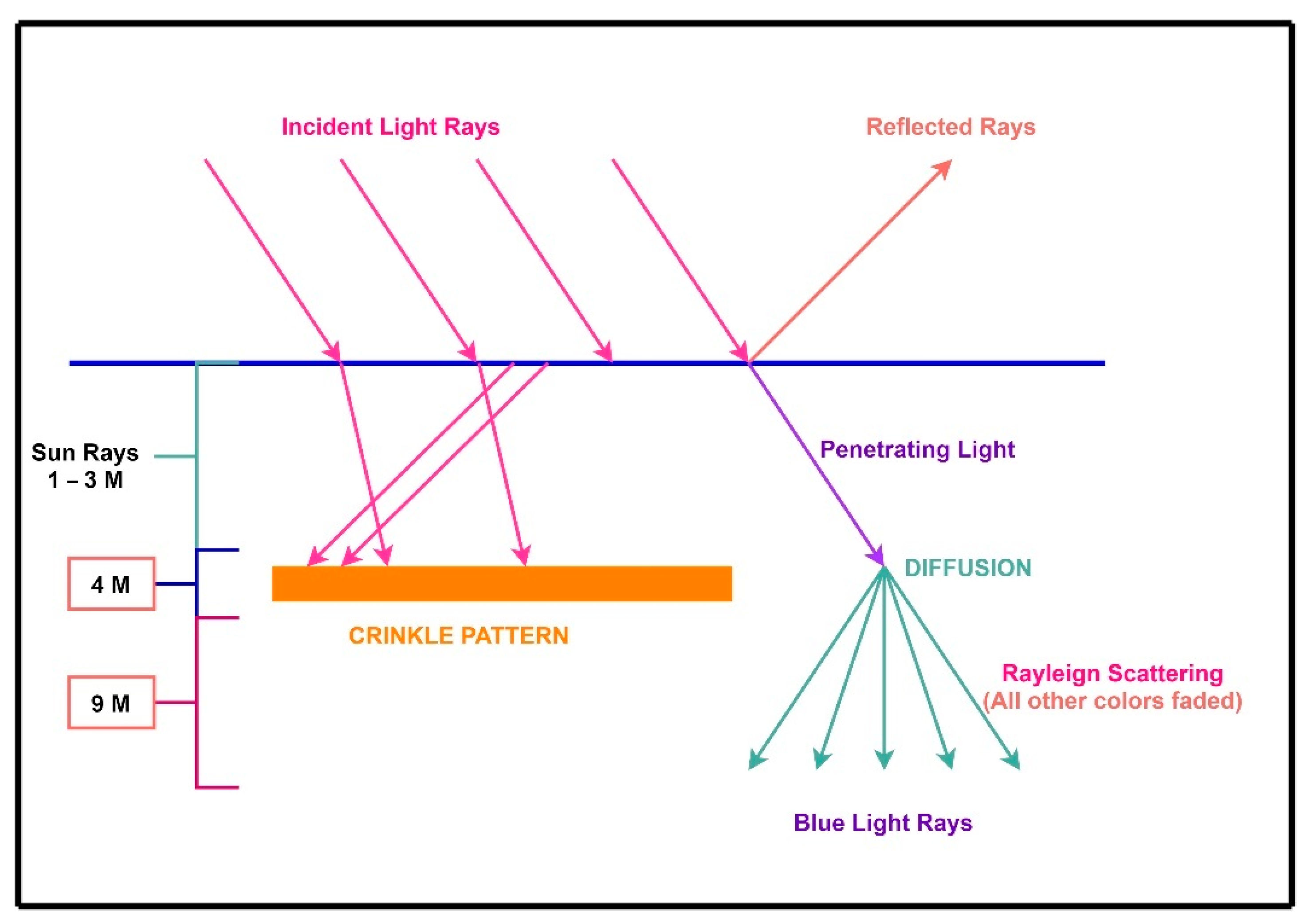
In this segment, a few challenges existing in underwater images, like light absorption and the effect of an implicit marine structure, are discussed. White [6] suggests that marine structure strongly affects light reflection. The water influences the light to either create crinkle patterns or to disperse them, as shown in Figure 2. Water quality such as sprinkling dust in water [7] also regulates and determines the features of water filtration. Moreover, the transmitted light is partly horizontally polarized and partly penetrates the water vertically. A vertical polarization enables the object to be less shiny, in turn enabling to retain dark colors which would have been marginalized otherwise.

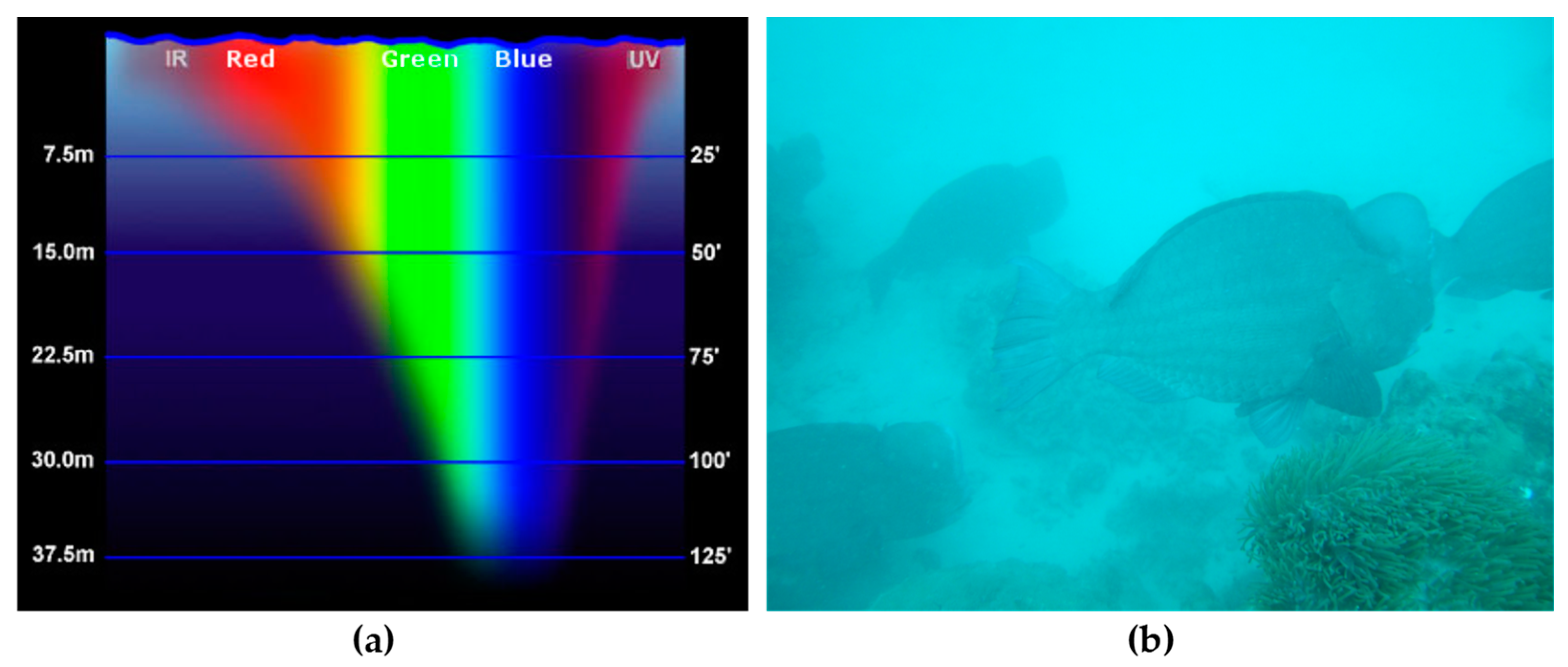
The density of the medium also plays a vital role in lowering the resolution of the underwater images. The density of water, which is 800 times that of air, induces light to be partly reflected when it travels from the air to water. As we move deeper into the sea, the amount of water entering the camera also decreases. This causes deep-sea images to look darker. Moreover, colors drop off systematically as a function of wavelength with depth. Since color is marked by a band of wavelengths, color degradation occurs with imaging depth.

Table 1. The Wavelength of Different Colours of Light.

Wavelength (m)	Color of Light
380–450 × 10−9	Violet
450–495 × 10−9	Blue
495–570 × 10−9	Green
570–590 × 10−9	Yellow
590–620 × 10−9	Orange
620–750 × 10−9	Red

shows the wavelength of different colors in the spectrum. The phenomenon of color dropping can be explained by considering a beam of light entering the sea/water [8]. As light enters the heavier medium (water), the light gets scattered. This phenomenon is referred to as backscattering in the area of photography where the rays of light are reflected back in the direction of the origin of light. Torres-Méndez and Dudek [9] report that, at a depth of 3 m, all the red color vanishes (highest wavelength). At the depth of 5 m, the orange color begins to fade. On moving deeper to 5 m, the orange color is completely lost and yellow becomes more vulnerable [10,11]. That also fades off at a depth of about 10 m, followed by green and purple disappearing further down the water level. Thus, the shorter the wavelength of the color, the longer the distance it travels. This results in a phenomenon where the color with the shortest wavelength dominates the image. [12] Blue has the shortest wavelength and a domination of blue color gives the image a low brightness. This paper mainly aims at the reconstruction of underwater images which are caused due to the poor lightening and dust in the deep-water bodies. The algorithm adopted for the removal of noise from the image bypasses the image through a trigonometric bilateral filter. Later, the images are enhanced by applying CLAHE. The experimental analysis and results are discussed in the following sections.

Generally, an image taken underwater always degrades in quality. It loses the true tonal quality and contrast necessary for distinguishing the image’s subject. When neighboring objects have very small differences in pixel intensity values, the situation becomes more difficult. This situation significantly complicates the task of extracting finer details from the data and degrades the performance of the algorithms used to extract information from images. As a result, there is a pressing need for underwater images to be processed in such a way that they accurately represents their tonal details. Underwater imagery is used for a variety of purposes, including the investigation of aquatic life, the assessment of water quality, defense, security, and so on. As a result, images or videos obtained to accomplish these objectives must contain precise details.

The purpose of this research is to develop an improved enhancement technique that is capable of operating in a variety of conditions and employs a standard formulation for evaluating the quality of underwater images. In this work, a hybrid solution is proposed. By training a deep learning architecture on image restoration techniques, a function for image enhancement is learned. A dataset consisting of pairs of raw and restored images is used to train a convolutional network, which is then capable of producing restored images from degraded inputs. The results are compared to those obtained from other image enhancement methods, with the image restoration serving as the system’s ground truth.

2. Related Work

A large number of underwater image processing methods have been discovered over the last two decades. Different approaches have been considered, e.g., inversion of the light propagation phenomenon, colour filtering, frequency filtering, etc. In this study, we propose to expose approaches based on colour filtering methods utilising the physical model on the one hand and colour consistency methods allowing unsupervised processing on the other. These methods rely on an adjustment of the luminance of the pixels of the image on each of the colour channels to improve the contrast and colours of the image [13]. Existing methods of processing by the physical model require knowing one or more references, allowing the establishment of the processing chain, as well as some knowledge on the conditions of acquisition. Chromatic adjustment methods are unsupervised but provide a chromatic correction that is not necessarily in keeping with reality. The goal is therefore to reconcile these two aspects, namely unsupervised and chromatic adjustment based on the physical model and the four methods that have caught our attention because they provide particularly good correction results [14].

Several methods based on the propagation model exist. Based on an estimate of the attenuation, they use controlled acquisition conditions. These systems make it possible to estimate the spectral attenuation and diffusion coefficients necessary for the model either by having reference in the image or by using more elaborate specific systems than the simple camera. This section presents two methods corresponding respectively to each of these two categories [15].

2.1. Underwater Image Correction Based on Spectral Data

In [16], the authors propose a correction method based on the attenuation coefficient. The estimation uses the reflectance values of a grey reference target in the images. This object, named Spectralon, is a plastic surface that strongly reflects light in a Lambertian reflection [16]. However, the camera’s properties and position are known. The luminance reaching the spectral is known as well as the value of the luminance reaching the camera for each of the three chromatic channels. The camera is positioned vertically on the ocean floor. So, the water column size corresponds to depth. The luminance received by the camera is thus written as a function of depth [17].

• The photographic seabed has a Lambertian reflection.
• The spectral receives as much light as the surrounding environment.
• The camera has stable sensitivity curves with respect to illumination variations.

With these elements, the attenuation coefficient can be expressed as a function of depth and luminance. The reflectance of an object is the ratio of the incident (incoming) Lin to the diffused (outgoing) Lout received by the spectral [18]. Peng et al. used Beer’s law to find the value corrected pixels after measuring the depth and attenuation coefficient. We could not replicate the acquisition campaign with the reference object. The visual quality of the correction is good judging by the results. However, the study only looks at clear water and shallow photographs. High turbidity of the water may distort the estimation of the attenuation coefficient and background luminance. This method also necessitates a mastery of acquisition (illumination, depth, position of the camera, etc.).

2.2. Underwater Image Correction with Polarization Filter

The second method [19] uses a light polarising filter. Inversion of the physical model poses the problem of estimating object-camera distance. Due to attenuation and diffusion, image visibility is minimal. This method is used to increase visibility. The authors suggest taking two images with different polarizations to gain more information. The authors first describe the camera-level image formation mechanism before implementing a treatment to compensate for diffusion and increase image visibility. This method relies not only on propagation inversion, but also on the acquisition system’s properties [20]. Using the light propagation model, the signal is the sum of the direct transmission D (attenuated light from objects) and the forward scatter (ambient light scattered in a direction close to the camera’s line of sight). So, the image signal is measured, and direct transmission is achieved. Forward scatter blurs the image. To compensate for this, the authors use a point spread function (PSF). In a plane image, a PSF accounts for distance, inverse Fourier transform, and spatial frequency [5].

A degraded image may affect both the human eye’s interpretation and the performance of a computer vision system. This section shows the phenomena that can affect the quality of the captured image at various stages of the scene acquisition chain. The chapter then describes methods for improving image quality [21].

2.3. Polarization

Underwater diffusion is polarised. The method uses these effects to compensate for visibility loss. An incidence plane is formed by a ray from a light source and the line of sight. Backscattered light is polarised parallel to this plane. As a result, natural underwater backscattering is partially horizontally polarised [22]. The scene is acquired through a polarising filter to measure the polarisation components. Because backscattering is polarised, its intensity varies with the filter’s orientation. Backscattered light transmittance reaches maximum values Bmax and Bmin for two orthogonal orientations. Two linear polarisation components result [23].

When using a polarizer, the image intensity is a cosine function of the orientation angle. The visibility enhancement algorithm compensates for the haze effect caused by the broadcast [24].

2.4. Total Variation Model

The image’s local characteristics determine its global regularity. Total variation refers to this regularity and is the sum of the image’s local gradients, as observed in the case of additive noise. Looking for the image creates image noise. Total variation is a regularisation term that allows discontinuities along sufficiently regular outlines to be penalised. Less variation in the image is achieved by increasing the denoising force [25]. Its disadvantage is that the textures can be considered noise and erased. Yang [26] noticed stairwell effects. This method can also be used to restore images degraded by fuzziness. The “Total Variation Model” method is a subset of Bayesian approaches.

2.5. Bayesian Approaches

For an image, the posterior distribution is expressed as a Bayes formula. Denoising increases this likelihood. The likelihood is known and determined from the model of data formation. The maximum likelihood (ML) estimate seeks to maximise the likelihood. It is simpler to estimate the log of this probability product. In general, maximisation involves finding an image that meets the probability density of a Gaussian noise. The prior can be taken into account in MAP estimation. The MAP is found by applying the logarithmic function to the Bayes formula [27]. They are often used to find prior probabilities. So, the image is an arrangement of atoms in various energy states, the grey levels. Only its neighbours determine an atom’s state. The Hammersley–Clifford theorem expresses this probability as the sum of potential functions computed on cliques (neighbourhoods), selecting potential functions (differential operator, for example) a priori [28]. There are two methods for determining the MAP [19]:

• Fast deterministic algorithms that may not converge to the global minimum. As an example, we discuss gradient descent and its variants.
• Slow stochastic algorithms that find a global minimum.

2.6. Transformed into Wavelets

Wavelets were invented in the early 1980s to solve a problem with the Fourier transform that prevented locating the signal’s frequencies in time. In order to recover the image without noise, the coefficients cmn and jo mn must be kept significant [29]. To recover the coefficients of interest to analysts, a threshold must be found to detect the noise coefficients, for which many methods exist (strong, soft thresholding). Other methods in the same family (time-frequency representation) include curvelet and contourlet. In addition to noise issues, the image may lose contrast [30].

2.7. Hazing Methods

Noise removal in images is an active area of research. Removal of haze by using a solo color-based framework was introduced by Fattal [31]. This method did not produce the required results in heavily hazed images due to its difficulty to ascertain the color lines. Lu et al. [32] suggested a method to enhance the underwater images of shallow oceans by estimating the ambient light in an image. The highlighted regions are removed by applying a bilateral filter-based de-flicker filter. The method could successfully reconstruct the color of images when particle sediments were of moderate size. The method could not, however, remove the hazy scatters in the image.

Later, Serikawa and Lu [33] introduced a de-hazing method that smoothens the depth map using an improved trigonometric filtering de-hazing algorithm. A complete framework for pre-processing underwater images was proposed by Arnold et al. [34]. The noise in underwater images could be removed using this method which involves a framework with a mixture of de-convolutional networks. To oppose lighting indifference, attenuation, backscattering, and contrast equalization were applied. As backscattering has a minimum change in value in space, this method plays a vital role. The method removes primary noise produced by back-scattering [35]. It is followed by a distance-dependent exponential light attenuation function to remove the remaining noise in the image. The detection of edges in the images is further improved using an adaptive smoothing filter.

Torres-Mendez and Dudek [7] noted that the color of images can be enhanced by considering it as an energy minimization problem on learned attributes/constraints. The model uses a stochastic process called the Markov random field (MRF) which captures the characteristics of the training data. This helps to learn a marginal probability distribution which is later used on the input images. Belief propagation (BP) infers the color correction on each pixel of the depleted image.

Belief propagation is an algorithm used to create inferences on graphical methods by calculating the probability distribution of variables. However, this algorithm fails in terms of accuracy due to the statistical inconsistency of the training set leading to a poor value of parameters, such as variance, iterations, and pixel difference of the MRF. Chongyi Li [36] presented the first comprehensive perceptual study and analysis of underwater image enhancement using large-scale real-world images. An underwater image enhancement benchmark (UIEB) was constructed which includes 950 real-world underwater images, 890 of which have the corresponding reference images. Qingbo [37] proposed a transmission-aware nonlocal regularization to avoid noise amplification by adaptively suppressing noise and preserving fine details in the recovered image.

3. Proposed Method

In our method, we address two main issues in underwater images, namely noise in the image due to the scattering of light and poor contrast of the image due to low lighting. The noises in an image can be removed in several ways. The most used method of noise removal includes the filtering method, anisotropic diffusion, based on nonlocal averaging of pixels, wavelet transforms, block matching algorithms, deep learning [38], etc. The dataset used for this experiment is taken from the underwater surveillance database of airis4D (airis4d.com, accessed on 22 May 2021). The most effective way of noise removal is by convolving the image with filters. These filters are mainly low pass filters. A low pass filter is also called a blurring or smoothing filter. The filters can be mainly of two types, linear and non-linear. A linear filter is considered to be more efficient in noise removal compared to a non-linear filter. The best example for a linear filter is the Gaussian filter which works on the Gaussian function.

The Gaussian filter has the advantage that its Fourier transform is also a Gaussian distribution centered around zero frequency. This is referred to as a low pass filter as it attenuates the high-frequency amplitudes. A bilateral filter on the other hand is an edge-preserving filter that replaces each pixel value with the average intensity of its neighboring pixel values. In the proposed method, a bilateral filter with a gaussian trigonometric function is used. This makes the computational complexity of O(N) which is more efficient than the state of art bilateral filtering methods. A non-linear low pass filter on the other hand is a filter whose output is not a linear function to its input. This includes the noise in the domain continuous and discrete as well. Examples of non-linear filters include the median filters, rank-order filters, and Kushner–Stratonovich filters. Other low pass filters include the Butterworth low pass filter, ideal low pass filter, etc. To remove the dust from the high pass filtered image, we introduce a convolutional neural network. To train the network, we create and use a synthetic dataset of 15,000 rainy/clean and dust/clean image pairs. Finally, the denoised high pass filtered image is the resultant dust removed image. CLAHE is applied to remove partial noises, thus improving the contrast of the image.

The proposed method uses the deep learning method to remove the noise and haze from underwater images. The proposed method is said to outperform the existing method based on its run time complexity and increased resolution of the reconstructed image. The computational complexity of the traditional bilateral filter is O(N²). The proposed method applies a trigonometric filter which has a complexity of O(N) This proves that it is more efficient than the state-of-the-art bilateral filtering methods. The noise in the underwater images caused by particles such as dust, sediments, and haze is removed by passing the image through a convolutional neural network (CNN).

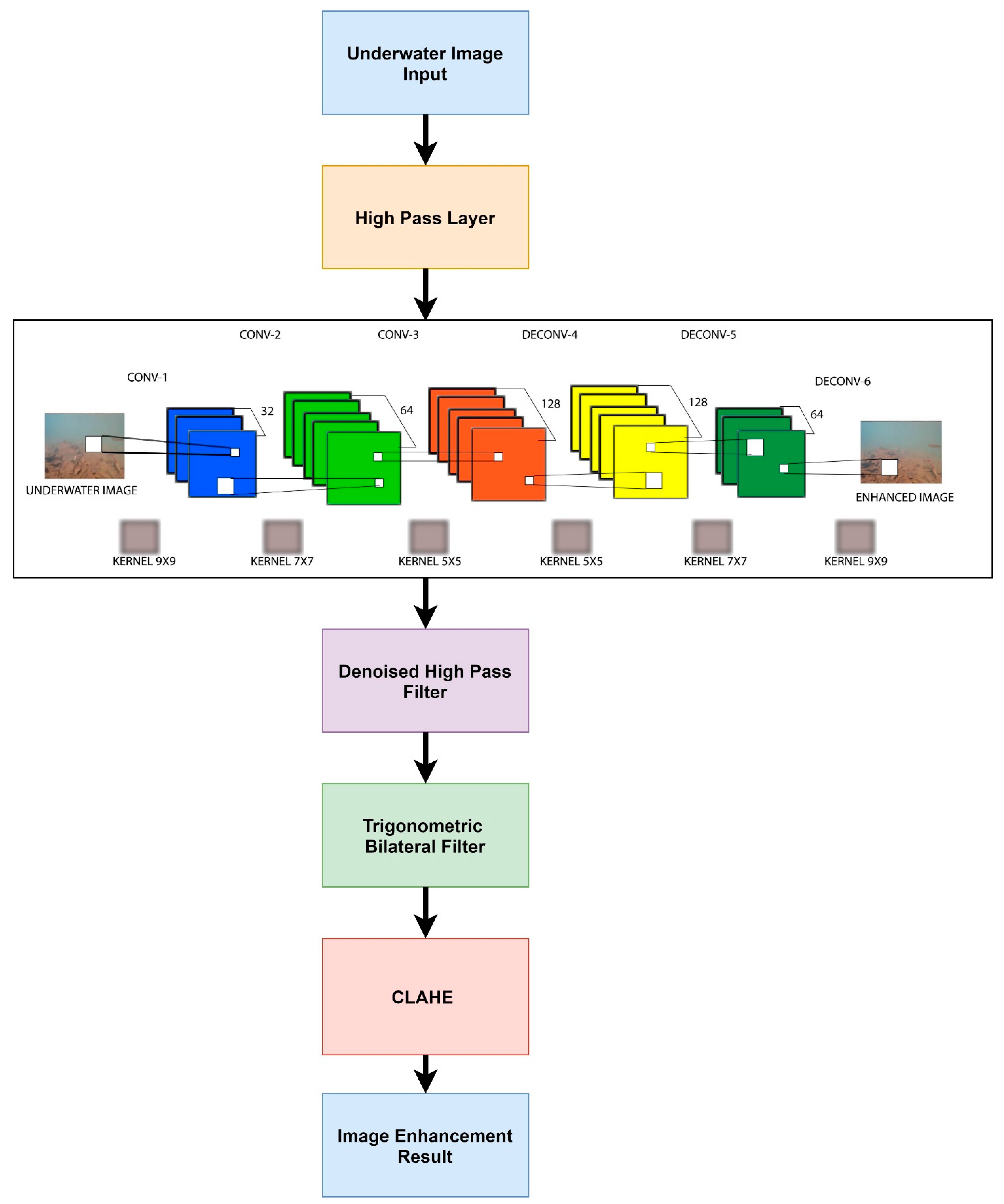
Figure 3 describes the schematic representation of the proposed framework. In the figure, the input is first passed to a high pass filter layer. For accomplishing this, the image is first converted to its frequency domain. The high pass filter makes the image appear sharper, emphasizing the fine details of the image by using a different convolutional kernel. The CNN is used to remove the unwanted noise in the image. The images that are considered for the noise removal are mainly 3-dimensional images. The images are fed to a convolutional neural network for the removal of noise. The CNN architecture consists of a low pass filter for the process of convolution. The size of the filter depends on the sigma σ (standard deviation) of the image (ideally the value of sigma is taken as 1). The filter size is calculated as 2 × int(4 × σ + 0.5) + 1. This computes the filter size to be 9 × 9. The filter is computed based on the bilateral trigonometric method. The feature map which is produced by sliding the filter over the input image is the dot product taken between the filter and the parts of the input image with respect to the size of the filter. In the proposed method, the network consists of 3 convolutional layers. The first layer consists of the input image of size 176 × 320 × 3. At each layer, the image is convolved with the filter of size 9 × 9. The activation function used for the proposed method is ReLu, which replaces all negative values of the matrix as zero. The images also undergo the process of padding in-order to retain the size of the original images. The image is then passed through a denoised bilateral filter which reduces noise in the image through a blurring effect. It replaces the intensity of each pixel in the image using the weighted average of its neighboring pixels. This weight is based on a Gaussian distribution. The last phase of the network is to apply CLAHE which improves the lost contrast of the image due to noise removal. The resultant image is an enhanced and noise-removed image. A detailed theory of the proposed method is described below.

We have used the method to enhance underwater surveillance videos to get clearer images for analysis. For this purpose, the video is first converted into frames and a trigonometric noise removal function [39] is applied as described in Section 3. The images are finally enhanced using the CLAHE algorithm described in Section 3. The frames are then put back to obtain the video as the result.

3.1. Noise Removal

The noise present in the images is eliminated by using a trigonometric filter. This filter uses a combination of bilateral filters applied on a Gaussian function. The edge-preserving bilateral filter includes a range filter other than a spatial filter. This enables to avoid the averaging of nearby pixels whose intensity is equal to or close to that of the pixel of interest.

As the range pixel operates on pixel intensities, it makes the process of averaging nonlinear and computationally better, even if the spatial filter is large.

In this paper, we have used trigonometric range kernels on the Gaussian bilateral filter. The general trigonometric function is in the form of f(s) = a₀ + a₁cos(γs) + … + a_Ncos(Nγs). This can be expressed exponentially as

$$\mathrm{f}(\mathrm{s})={{\displaystyle \sum }}_{\left|n\right|\le N}^0{c}_n{e}^{jn\mathsf{\gamma }\mathrm{s}}$$

(1)

Coefficients $c_n$ must be real and symmetric since f(s) is real and symmetric. The trigonometric kernel applied on the bilateral filter is based on the raised cosine kernel function. Moreover, f(s) have some additional properties to qualify as a valid range kernel. This includes that the function f(s) should be positive or non-negative and must also be monotonic. This ensures that it behaves like a spatial filter in a region having uniform intensity. The raised cosine of the trigonometric property helps to keep the properties of symmetry, nonnegativity, and monotonicity. This is explained by Equation (2).

$$\mathrm{f}(\mathrm{s})={[\cos \mathsf{\gamma }\mathrm{s}]}^N\left(-\mathrm{T}<\mathrm{s}<\mathrm{T}\right)$$

(2)

A bilateral filter is a non-linear filter that smoothens the image by reducing noise and preserving the sharp edges of the image. The intensity of every pixel is replaced by the average weighted value of the intensity of its neighboring pixels in an image. The weights are calculated based on a Gaussian distribution.

There are two parameters that a bilateral filter depends on, σs and σr. The σr is the range parameter and σs is the spatial parameter. The Gσr represents the range kernel Gaussian function which is used for smoothing the differences in intensity value between neighboring pixels. Gσs is the Gaussian function for smoothing the differences in coordinates in the image. The dependency of σs and σr on the bilateral filter can be explained in terms of range parameters and spatial parameters. The widening and flattening of the range Gaussian Gσr lead to more improved accuracy in the computation of Gaussian convolution by the bilateral filter. This is proportional to the distance parameter σr. Increasing the σs spatial parameter smoothens larger characteristics. In Equation (1), the intensity of pixels is represented by a function of a and y.

A bilateral filter has a major disadvantage. If the product of weights in the bilateral filter computes to zero or close to zero, then no smoothening or removal of noise occurs. This is overcome using a Gaussian-based trigonometric filter which uses a raised cosine function with the unique properties of symmetry, nonnegativity, and monotonicity. The bilateral trigonometric filter is defined as (3).

f(x) = 1/(ω(x)) ∫G_σs (y)G_σr (f(x − y) − f(x)) f(x − y)dy

(3)

where

ω(x) = ∫G_σs (y)G_σr (f(x − y) − f(x))dy

(4)

and ω is the normalization coefficient.

In our experiment, we assume the intensity values of f(x) are varied in the interval [−T, T], i.e., the difference in the intensity among neighboring pixels (σr). The Gaussian function of σr, Gσr, can be approximated by raised cosine kernels as (5).

$$\underset{N\to \infty }{\lim }\cos {(\frac{\mathsf{\gamma }\mathrm{s}}{\sqrt{N}})}^N=e^{\frac{-{\mathrm{s}}^2{\mathsf{\gamma }}^2}{2{\mathsf{\rho }}^2}}$$

(5)

for all −T ≤ s ≤ T, where γ = π/2 T and ρ = γσr (normalized radiance of a scene point).

Equation (3) leads to the important conclusion that the variance of the output Gaussian function and raised cosine values are positive and unimodal for all values of N ranging from [−T, T]. Here, T refers to the difference in intensity of a source pixel and its neighboring pixel. In the above equation ‘s’ ranges from the minimum to maximum value of the pixel in the image. ‘γ’ refers to π/2 times the difference in intensity of the image, ‘ρ’ refers to the normalized radiance of a scene point, and N refers to every pixel of the image where the Gaussian range function is applied.

3.2. Contrast Limited Adaptive Histogram—CLAHE

This method is applied on tiles, a small region in the image rather than the whole image. The variance in luminance or color that makes an object different from other objects within the same field of view is defined as a contrast. The intensity of an image is adjusted by the histogram equalization which helps in enhancing the contrast of an image. In the adaptive histogram equalization, every region of the image has its respective histograms thus causing every region of the image to be enhanced separately. This also enables the redistribution of the light in the image. The major advantage of AHE is that it improvises the local contrast and edge sharpness in every region of the image.

AHE mainly depends on 3 properties. Firstly, the size of the region, the larger the size of the region lower is the contrast and vice versa. Secondly, the nature of the histogram equalization determines the value of pixel, which is, in turn, dependent on its rank within the neighborhood. Thirdly, AHE causes over-amplification of noise in large homogeneous regions of the image as the histogram of these regions is highly peaked causing the transformation function to be narrow. The major disadvantage of using AHE over CLAHE is that AHE works on similar fog whereas a CLAHE could be applied over both similar and dissimilar fog images. The second drawback of AHE is that it uses a cumulative function that works only on gray-scale images whereas CLAHE works on both colored and gray-scale images.

CLAHE mainly depends on 3 parameters, namely block size, histogram bins, and clip limit. The block size represents the number of pixels considered in each block. For example, for a block size of 8 × 8, 64 pixels are considered. Eventually, the block size also affects the contrast of images significantly. The local contrast is achieved with smaller block size and the global contrast in the image is attained by larger block size.

For a low-intensity image, the larger the value of the clip limit, the brighter the image will be. This is because the clip limit makes the histogram of the image flatter. Similarly, the contrast of the image is increased when the size of the block is large as the dynamic range is higher.

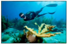
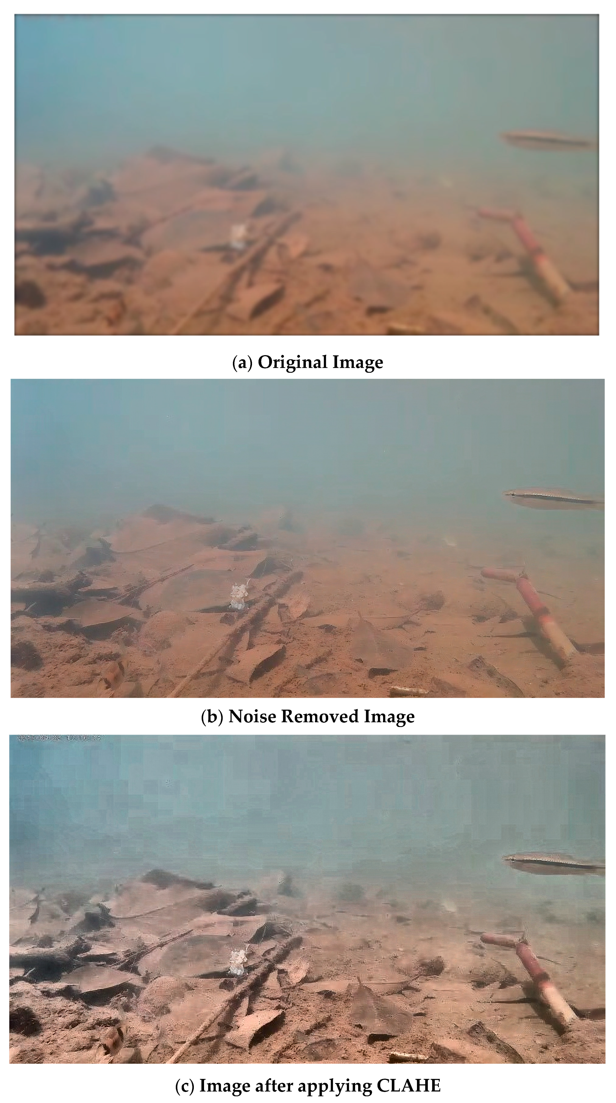
Figure 4 shows the reconstruction of an image by applying a Trigonometric filter. The first image (a) is the ground truth image. This image is taken from a video of underwater clipping. The SNR of Figure 4a is found to be 12.92. The second image (b) is the reconstructed image after passing the noise image through a bilateral trigonometric filter. The final image (c) is a contrast-enhanced image after applying CLAHE. The SNR of the reconstructed image is 20.38. This shows that the signal-to-noise ratio is higher in the reconstructed image when compared to the image with noise (S&P).

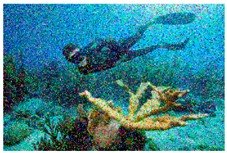
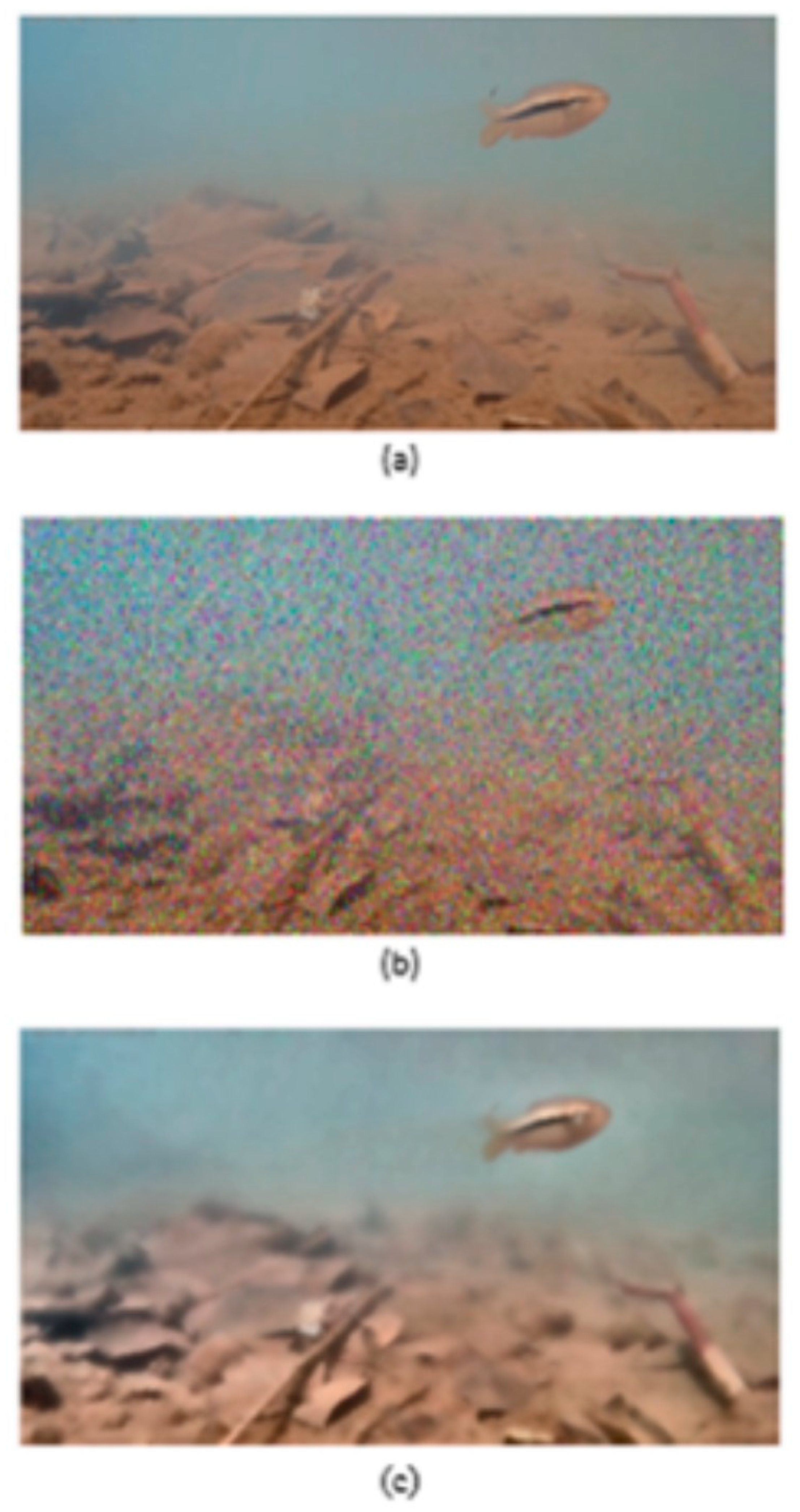
A similar example is shown in Figure 5 as well. The image in Figure 5 is another frame from the same underwater clipping. Here, the ground image has an SNR of 47.85. On applying salt and pepper noise to the image, the noise level increases, thus decreasing the SNR to 15.23. On applying the proposed method to Figure 5b, the signal strength is improved, bringing the SNR value to 17.8.

3.3. Metrics Used

The quality of an image is measured using the parameters namely, the signal noise ratio (SNR), mean squared error (MSE), underwater image quality measure (UIQM), and structural similarity index (SSIM).

The signal noise ratio (SNR) and mean squared error (MSE) of the reconstructed image and ground image was compared. The MSE of the reference image (ground truth image) is calculated with reference to the noise image and reconstructed image (target images). The SNR of the target image with comparison to the reference image is calculated as shown as (6)

SNR = 10 × R

(6)

where

R = Variance (v_ref)/MSE (v_ref, v_cmp)

(7)

Here, v_ref refers to the ground image or the reference image or the ground truth image and v_cmp refers to the reconstructed/noise image.

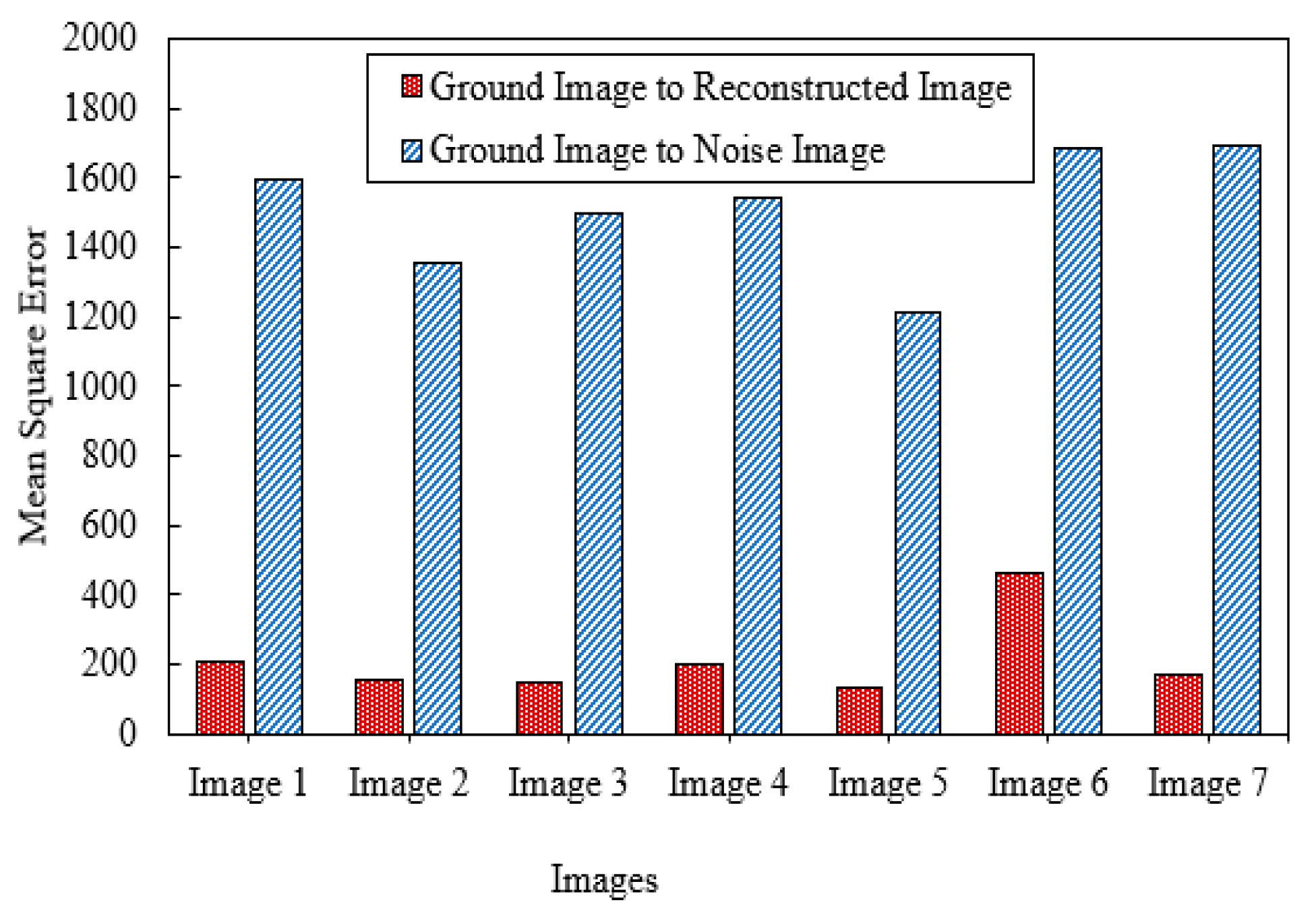
The MSE of the images are tabulated in

Table 2. Mean Squared Error (MSE) of Images.

Ground Image	Comparison	Mean Square Error (MSE)
Image 1	Ground Image to Reconstructed Image	203.8
	Ground Image to Noise Image	1598
Image 2	Ground Image to Reconstructed Image	152.23
	Ground Image to Noise Image	1358.65
Image 3	Ground Image to Reconstructed Image	147.8
	Ground Image to Noise Image	1496.1
Image 4	Ground Image to Reconstructed Image	197.2
	Ground Image to Noise Image	1543.9
Image 5	Ground Image to Reconstructed Image	131.33
	Ground Image to Noise Image	1211
Image 6	Ground Image to Reconstructed Image	458.9
	Ground Image to Noise Image	1683.11
Image 7	Ground Image to Reconstructed Image	168
	Ground Image to Noise Image	1691.57

. These images are different frames of underwater image clippings. It shows the error of the noise image and the reconstructed image with respect to the ground image. The noisy image is generated by applying salt and pepper noise of intensity 0.1. Figure 6 shows the plot of the MSE noisy image in relation to its corresponding reconstructed image.

A measure of the similarity between 2 images is given by the Structural Similarity Index (SSIM). The Image and Video Engineering Laboratory based at the University of Texas, Austin was the first one to coin the term. There are two key terms here, structural information and distortion. These terms are usually defined with respect to image composition. The property of the object structure that is independent of contrast and brightness is called structural information. A combination of structure, contrast, and brightness gives rise to distortion. Estimation of brightness was undertaken using mean values, contrast using standard deviation, and structural similarity was measured with the help of covariance.

SSIM of two images, x and y can be calculated by:

$$\mathrm{SSIM}\left(\mathrm{x},\mathrm{y}\right)=\frac{\left(2{\mathsf{\mu }}_{\mathrm{x}}{\mathsf{\mu }}_{\mathrm{y}}+{\mathrm{c}}_1\right)\left(2{\mathsf{\sigma }}_{\mathrm{xy}}+{\mathrm{c}}_2\right)}{\left({\mathsf{\mu }}_{\mathrm{x}}^2+{\mathsf{\mu }}_{\mathrm{y}}^2+{\mathrm{c}}_1\right)\left({\mathsf{\sigma }}_{\mathrm{x}}^2+{\mathsf{\sigma }}_{\mathrm{y}}^2+{\mathrm{c}}_2\right)}$$

(8)

In Equation (8), the average of x is μ_x and the average of y is μ_y. σ2x and σ2y gives the value of variance. The covariance x and y are given by σxy. c₁ = (k1L2), c₂ = (k2L2) are constants. They are used to preserve stability. The pixel values dynamic range is given by L. Generally, k1 is taken as 0.01, and k2 is given by 0.03.

Underwater image quality measure (UIQM) has also been taken into consideration to quantify parameters like underwater image contrast, color quality, and sharpness. This umbrella term consists of three major parameters to assess the attributes of underwater images, namely, underwater image sharpness measure (UISM), underwater image colorfulness measure (UICM), along with underwater image contrast measure (UIConM). Each of these parameters is used to appraise a particular aspect of the degraded underwater image carefully. Altogether, the comprehensive quality measure for underwater images is then depicted by

$$\mathrm{UIQM}={\mathrm{c}}_1\times \mathrm{UICM}+{\mathrm{c}}_2\times \mathrm{UISM}+{\mathrm{c}}_3\times \mathrm{UIConM}$$

(9)

Equation (9) relates all three attributes mentioned effectively. The selection of the parameters c₁, c₂, and c₃ are purely based on the parameters’ application. As an illustration, consider UICM. This parameter is given more weightage for applications that involve image color correction while sharpness (UISM) and contrast (UIConM) have more significance while enhancing the visibility of the images. UIQM regresses to an underwater image quality measure when these two parameters achieve null values.

4. Discussions and Result Analysis

Underwater images contain disturbances which are mainly caused by the noise in the image due to the scattering of light. The poor contrast in the image due to low lighting while the image is captured. This is reduced to a great extent by the proposed method by applying a trigonometric filter and CLAHE. The resultant image is an enhanced and noise-removed image. The results attained using the proposed method are compared using the metrics of SNR, SSIM, MSE, and UQIM of the images. The experimental results show that the proposed method performs better in removing haze-like scatters and dust-like scatters.

The experimental results using the proposed produces a more contrast and clear image compared to the ground image. SNR, which is used to define the quality of an image, is used as a metric to validate the images. The greater the value of SNR, the more improved the quality of the image.

Table 3. Comparison of SNR of Images.

Images	SNR
	Ground	Image with a Noise of 0.1 S&P	Reconstructed
Image 1	13.08	12.4	16.69
Image 2	14.6	13.6	15.64
Image 3	17.5	16.36	18.56
Image 4	37.55	24.95	28.22
Image 5	40.58	25.34	26.54
Image 6	47.85	15.23	17.8
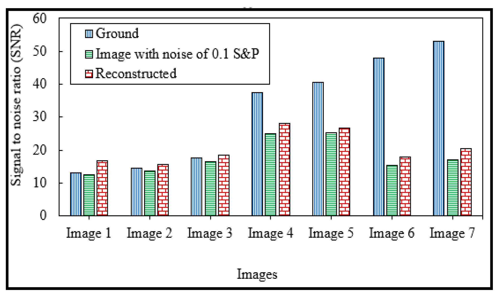
Image 7	52.92	16.98	20.38

provides the complete analysis of SNR values of the ground image and the image after its reconstruction using the proposed method using the trigonometric bilateral filter. The table explains that the image taken for the test has an improved value of signal compared to its noise images. From the results, it can be inferred that the SNR value of the noise image is less than the corresponding reconstructed image. The decreased value of SNR proves the increased noise in the image. From the statistical data in Table 3, it can be inferred that for images 1, 2, and 3, the SNR of the reconstructed image is greater than the ground images. For raw images with SNR greater than 20, the signal in the reconstructed image is substantially lower when compared to the ground image. Thus, it is not able to reach the quality of the ground image. The grey line depicts the value of reconstructed and the orange line shows the SNR of noise images. Figure 7 plots the SNR comparison of the images. The SNR of the ground image is shown using a blue line. The graph shows that the SNR of the noise image is less than the reconstructed images, thus showing more noise content in it. The blue line is the SNR of the ground image, orange is the SNR of the noisy image (0.1 salt and pepper noise is applied), and the grey line is the reconstructed SNR of each image. From the graph, for image 1, the SNR of noise is 12.4, and the reconstructed image by applying the proposed method has an SNR of 16.69. This variation helps to understand the efficiency of noise removal in the images. Thus, the proposed method of noise removal using the trigonometric bilateral filter and contrast enhancement using CLAHE is highly effective and efficient.

The proposed method was compared with the existing algorithm stated by Li [37]. A comparison of the MSE, SNR, and SSIM is shown in

Table 4. Image Quality Reference.

Method	MSE (×103)	PSNR (dB)	SSIM
Proposed Method	0.4589	17.8	0.8712
Bluriness Based [40]	1.5826	16.1371	0.6582
Dive+	0.5358	20.8408	0.8705
Fusion Based [41]	0.8679	18.7461	0.8162
GDCP [39]	3.6345	12.5264	0.5503
Histogram Prior [35]	1.6282	16.0137	0.5888
Red Channel [11]	2.1073	14.8935	0.5973
Regression Based [42]	1.1365	17.5751	0.6543
retinex-based [43]	1.3531	16.8757	0.6233
Two-step based [44]	1.1146	17.6596	0.7199
UDCP [16]	5.13	11.0296	0.4999

. The reconstructed image is said to be closer to its ground image if it has a lower MSE and higher PSNR value, while a higher SSIM score means that the result is more similar to its reference image in terms of image structure and texture. Structural similarity index measure (SSIM) is a metric used to compare the perceived quality of an image. It helps to define the similarity between two images. Table 4 explains that the proposed method has a lower MSE and higher PSNR value compared to state of art methods.

Table 5. SNR Comparison of an Image with Different Intensity of Noise.

S&P Noise	Noise Image	Reconstructed Image
0.1	SNR = 12.4	SNR = 16.69
0.2	SNR = 11.9	SNR = 17.63
0.3	SNR = 11.44	SNR = 18.49
0.4	SNR = 11.11	SNR = 19.55
0.5	SNR = 10.8	SNR = 21.67
0.6	SNR = 10.55	SNR = 23.50
0.7	SNR = 10.42	SNR = 26.53
0.8	SNR = 10.26	SNR = 28.82
1	SNR = 10.01	SNR = 31.35

shows the image reconstruction by applying different levels of noise. The image is mixed with salt and paper noise. The third column shows the corresponding reconstructed image of the noise image using the proposed method. It can be adduced that, as the noise intensity varies from 0.1 to 1, the SNR value of the noise image decreases, thus showing more content of noise than the signal. Moreover, upon analyzing the reconstructed image, it can be noticed that the SNR value increases, which conveys that the signal is reconstructed from the noised images. This shows the efficiency of our method.

The other inference from this experiment is that even though the noise level in the image increases, the perception of the reconstructed image is good to some extent. Perception is defined as the pattern formed by the visual centers of the brain after an image reaches the human eye. An image can be perceived differently by different humans.

It is the process of what one sees, organizing it in the brain, and making sense of it. Perception is the ability to see from the senses. It is how an individual sees, interprets, and understands visual data. From our experiment, we perceive that after the noise of more than 50% (S&P = 0.5) is applied, the perception of the corresponding reconstructed image starts to decrease. From Table 5, we infer that the perception of the reconstructed image of 0.1 noise is higher than that of 0.2, 0.3, and so on. The proposed method can reconstruct images up to a noise level of 0.5. The reconstructed images of noise higher than 0.6 have a very low level of perception, even though the signal strength is higher. Thus, the perceptional view decreases even though the signal strength is higher.

Table 6. Average Runtime for Different Image Sizes (In Second).

Method	1280 × 720	640 × 480	500 × 500
Proposed Method	1.598	0.6012	0.5889
Bluriness Based [40]	146.0233	47.2538	37.0018
Fusion Based [41]	1.8431	0.6798	0.6044
GDCP [39]	9.5934	3.8974	3.2676
Histogram Prior [35]	16.9229	5.8289	4.6284
Red Channel [11]	9.7447	3.2503	2.7523
Regression Based [42]	415.4935	167.1711	138.6138
Retinex Based [43]	2.1089	0.8829	0.6975
Two-step based [44]	1.0361	0.4391	0.2978
UDCP [16]	9.9109	3.3185	2.2688

shows the average run time required for removing noise in images using the existing algorithms stated by Li [37]. The statistics show that the proposed algorithm works better than the existing methods. This experiment was performed in different sizes of the images like 1280 × 720, 640 × 480, and 500 × 500. The results show the outstanding performance of the proposed algorithm.

Table 7. Evaluation Metrics Comparison of UIQM Scores.

Method	1280 × 720	640 × 480	500 × 500
Proposed Method	2.41	2.85	3.23
Bluriness Based [40]	2.12	2.51	3
Fusion Based [41]	2.11	2.80	3.22
GDCP [39]	1.98	2.66	3.15
Histogram Prior [35]	2.39	2.65	3.05
Red Channel [11]	2.21	2.69	3.15
Regression Based [42]	2.33	2.81	3.10
Retinex Based [43]	2.1	2.55	3.01
Two-step based [44]	2.02	2.32	3.18
UDCP [16]	2.3	2.76	3.20

shows the UIQM SCORES of images using the existing algorithms stated by Li [37]. The proposed method has a greater UIQM value compared to the existing methods for different image sizes used for the testing purpose.

5. Conclusions

The algorithm proposed in this paper is a tool for increasing the quality of marine optical images. The proposed method enhances the image by reducing the noise using a bilateral trigonometric filter. Finally, the contrast of the image is improved using CLAHE. The noise in the image, due to back scattering, the presence of large particles, and haze, is addressed. This model provides a high SNR value for the reconstructed images for images with SNR values less than 25. Moreover, the perception of the reconstructed image seems to be good up to a noise intensity of 0.5. Nevertheless, during the experiments, we found that the edges of the objects present in the image were not clear. Some of the images were detected with false edges and some details of the images were lost after applying the Gaussian filter. In addition, determining the parameters of CLAHE is a challenging task. This is one of the major disadvantages of applying CLAHE for improving image contrast. Thus, in the future, we would work on further improving the clarity of the image by concentrating on the image sharpness and the determination of parameters of CLAHE, thus increasing the resolution of the images further.