Fluctuating Characteristics of the Stilling Basin with a Negative Step Based on Hilbert-Huang Transform

Abstract

The violent fluctuation of hydrodynamic pressure in stilling basins is an important factor threatening the safety of the bottom plates of stilling basins, and plays an important role in the safe operation of stilling basins. In order to deeply understand the fluctuating characteristics of stilling basins, the fluctuating pressure signal of a stilling basin bottom plate is processed by the Hilbert-Huang transform method through a hydraulic model test. In this paper, three signal decomposition methods are used to decompose the pulsating pressure signal. A Hilbert transform is used to select the component with the best decomposition effect. The time-frequency-amplitude diagram of the pulsating pressure signal is obtained by Hilbert transform, and its time-frequency characteristics are discussed in depth. The analysis results are as follows: (a) the decomposition results from the CEEMD method are orthogonal and complete. The HHT method is suitable for processing fluctuating pressure signals. (b) With an increase in IMF decomposition order, the signal frequency band becomes narrow, the Hilbert spectrum amplitude decreases and the pulsating pressure energy decreases. The decomposition of the fluctuating pressure signal into components of different scales shows that the turbulence is composed of multiple scales of vortices, reflecting the vortex structure in the turbulence. (c) The jet impingement zone of the drop bucket stilling basin is near x/L = 0.075. The dominant frequency and marginal spectrum energy of the jet impingement zone are very prominent, and the marginal spectrum energy is mostly concentrated within 5.0 Hz. (d) At different drop height and different flow energy ratio, the fluctuation in the dominant frequency of fluctuating pressure decreases, the dominant frequency of the head of the stilling basin is larger, the dominant frequency of the middle and rear parts tends to be stable, and the dominant frequency is finally stabilized at about 1.0 Hz. This paper attempts to use the HHT method to process the fluctuating pressure signal, and the results provide a new discussion method for exploring the fluctuating pressure characteristics of hydraulic structures.

1. Introduction

Stilling basins with a negative step are a representative new type of energy dissipation building [1]. Compared with the conventional stilling basin, stilling basins with a negative step not only ensure a high energy dissipation rate, but also significantly reduce the bottom flow velocity of the stilling basin, and the resulting flood discharge atomization is very small [2]. Therefore, stilling basins with a negative step are widely used in water conservancy projects. Figure 1 shows a schematic diagram of a conventional stilling basin and a stilling basin with a negative step.

In recent years, the bottom plates of stilling basins in many high dam projects have been seriously damaged. This has been attributed to the fluctuation of hydrodynamic pressure on the bottom plates of stilling basins. The fluctuation of hydrodynamic pressure acting on the bottom plate of a stilling basin may cause the vibration of hydraulic structures and increase the possibility of cavitation erosion [3]. No matter what type of stilling basin, once resonance occurs, it will seriously threaten the safety of hydraulic structures [4]. Therefore, the study of fluctuating pressure characteristics of stilling basin floors has important engineering significance.

Pulsating pressure sensors are mostly used in the measurement of fluctuating pressure. The results of these measurements are random waveform graphs with irregular shapes. The analysis and calculation of waveform graphs are a significant research focus. In existing research, mathematical statistics and power spectrum analysis are the two most commonly used methods to study the fluctuating pressure characteristics in stilling basins [4].

The result of the measurement of fluctuating pressure is a random waveform with an irregular shape. It is very important to study this nonstationary signal. At present, the Fourier transform and wavelet analysis are the two most commonly used methods to study the fluctuating pressure in stilling basins [5]. However, fast Fourier transforms can only be analyzed in time or frequency domains and cannot express the time-frequency local properties of signals. Wavelet analysis depends on the selection of basis functions, and different selections of basis functions may lead to inconsistent analysis results [6].

In 1998, the Hilbert–Huang transform was created on the basis of the Fourier transform and wavelet transform. It is a research method created by Huang et al. [7]. This method breaks through the limitations of the Fourier transform, and at the same time has the advantage of the multi-resolution of the wavelet transform. This article attempts to use this signal processing method to study the spectral characteristics of pulsating pressure. It should be noted that this method is only an attempt and supplement to the pulsating pressure signal processing method, and does not attempt to replace the traditional spectrum analysis method.

The HHT method includes two parts: Empirical Mode Decomposition (EMD) and the Hilbert transform [7]. EMD is an empirical method, but the decomposition of this method is based on the inherent characteristics of the signal itself and does not require a windowing function, so it has good adaptability and completeness. The author compares the Fourier transform, wavelet analysis and the Hilbert-Huang transform from the aspects of whether the signal processing technology needs the basis function, whether it is suitable for nonlinear and non-stationary signals, and whether it has theoretical basis. The comparison results are shown in the

Table 1. Comparison of commonly used signal processing methods.

Comparison Item	Fourier	Wavelet	HHT
Basis	a priori	a priori	a posteriori adaptive
Presentation	energy in frequency space	energy in time-frequency space	energy in time-frequency space
Nonlinearity	no	no	yes
Nonstationary	no	yes	yes
Feature extraction	no	Discrete, no; continuous, yes	yes
Theoretical base	complete mathematical theory	complete mathematical theory	empirical

.

According to the comparison in the table, the HHT method can adaptively decompose the fluctuation of different scales in the signal, describe the time-frequency characteristics of non-stationary and nonlinear signals, and quickly capture the transient characteristics of the signal [8]. When dealing with non-stationary and nonlinear signals, the Hilbert–Huang transform is more suitable than the Fourier transform and wavelet transform.

Therefore, in the medical field, the HHT method is used to detect arrhythmia and changes in blood pressure. In the transportation field, the HHT method is used to detect the safety of highway bridges. In the aerospace field, the HHT method is used to analyze satellite data. The HHT method has high time-frequency resolution when processing nonlinear and non-stationary signals, but is also an empirical method. The current theory is not perfect and is still in the research stage. In this paper, the HHT method is used to study the rich information contained in the fluctuating pressure signal of the bottom plate of a stilling basin with a negative step. A new research method for signal processing of fluctuating pressure is added, which is of great value to theoretical research and engineering applications of bottom plate fluctuating pressure in stilling basins with a negative step.

In this paper, we attempt to use the above three methods to decompose the pulsating pressure signal, and select the best component for a Hilbert transform through the signal decomposition evaluation system. The Hilbert spectrum and Hilbert marginal spectrum of the characteristic points on the axis of the bottom plate of the plunge pool are obtained based on a Hilbert transform, and the time-frequency characteristics and amplitude distribution of the fluctuating pressure signal are obtained. Based on the above results, the energy distribution and main frequency variation of IMFs under different flow energy ratios are discussed. The applicability of the HHT method in fluctuating pressure signal processing of plunge pool bottom plates is discussed by comparing the results of the HHT method with that of a fast Fourier transform.

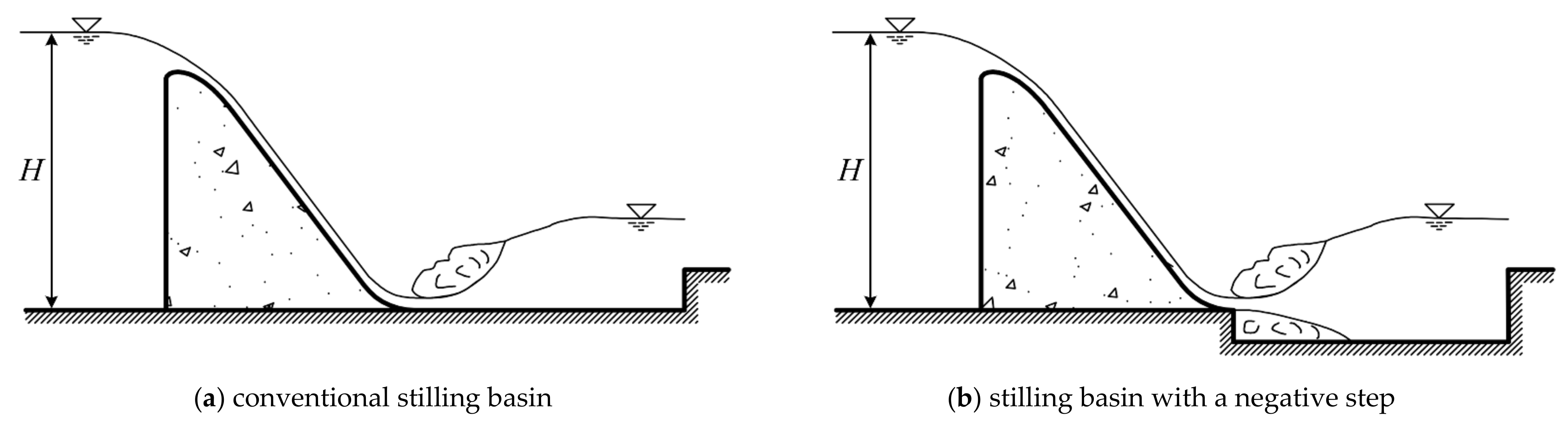
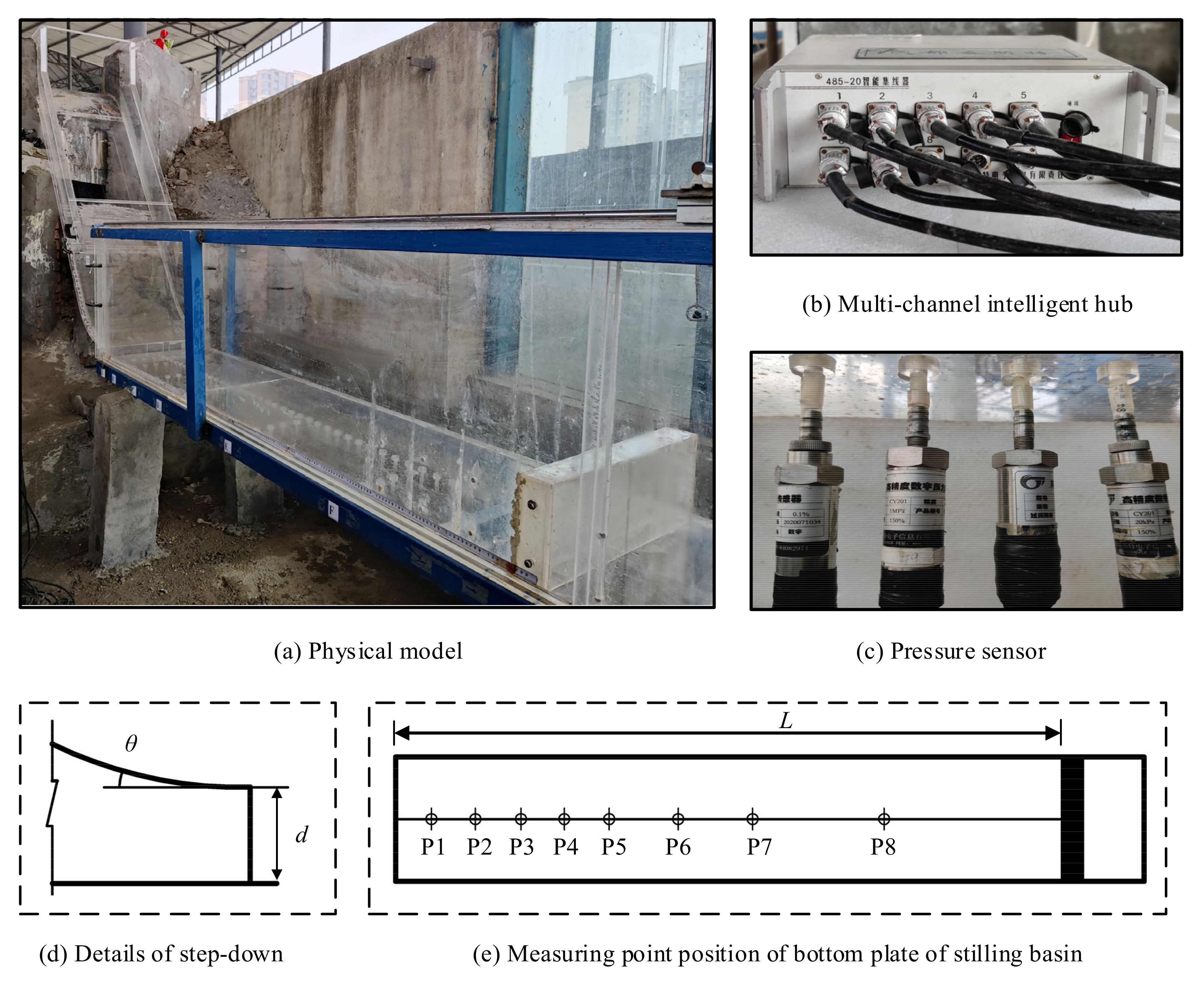
2. Physical Modeling and Experimental Setup

The experimental device consists of water weir, reservoir, spillway, stilling basin and circulating water source. The model is made of organic glass. The flow rate of the model is controlled by a thin rectangular wall weir with a precision of 0.1 mm. A SDA1000 high-performance digital sensor system was used to collect and process the fluctuating pressure. Instruments were calibrated before collection to ensure the reliability of the measurements. The sampling time was 4 min and the sampling frequency was 100 Hz. The measuring points were arranged along the center line of the bottom plate, the opening diameter is 2 mm, the interval is 5–10 cm.

Figure 2 shows the model layout. In order to measure the fluctuating pressure at eight points at the same time, eight sensors were inserted at the bottom of the stilling basin at the same time, and were connected to a multi-channel intelligent hub. The fluctuating pressure at eight points was measured by the instantaneous pressure sensor and transmitted to the computer through the hub at the same time. Figure 2a shows the overall layout of the physical model. Figure 2b shows the multi-channel intelligent hub. Figure 2c shows that some sensors are connected to the bottom of the stilling basin. Figure 2d is a detailed diagram of the stilling basin with the drop-sill, showing the drop-sill parameters: the height of the drop-sill (d), and the incident angle (θ).

In order to describe the position of pressure measuring points, a one-dimensional coordinate system was established, with the axis of the bottom plate of the stilling basin as the x axis. The original coordinate point was set at the intersection of the front end of the stilling basin bottom plate and the axis, and eight measuring points were arranged along the axis of the stilling basin.

Table 2. The measuring point position table on the central axis of the bottom plate of the stilling pool.

Number of Measuring Points	x/m	Number of Measuring Points	x/m
P1	0.025	P5	0.225
P2	0.075	P6	0.325
P3	0.125	P7	0.450
P4	0.175	P8	0.640

shows the positions of the eight measuring points on the bottom plate of the stilling basin.

In the model test, four experimental conditions were designed. In order to facilitate the description of different flow patterns, the dimensionless number–flow energy ratio k is introduced, which can reflect the hydraulic condition in the model. K is calculated by the following formula:

$$k=\frac{q}{g^{0.5}{H}^{1.5}}$$

(1)

where: q is unit discharge; H is the water level difference between upstream and downstream; g is the acceleration of gravity.

Table 3. Table of experimental conditions.

Test Plan	Q (L/s)	q	H (m)	k
a	30	0.06	131.12	0.0134
b	50	0.10	134.40	0.0223
c	70	0.14	136.88	0.0308
d	90	0.18	139.20	0.0403

calculates the flow energy ratio at different flow rates and different heads, where Q represents the upstream flow, q is the single-width flow, H is the difference between the upstream and downstream heads, and k is the flow energy ratio.

In this experiment, the conventional stilling basin was set as the control group. Four kinds of stilling pools were designed with different slam heights. The design of different stilling basin parameters is shown in

Table 4. Test plan of stilling basin with negative step.

Test Plan	d (m)	θ (°)
TP 0	0	0
TP 1	0.025	15
TP 2	0.050	15
TP 3	0.075	15
TP 4	0.100	15

, where d is the height of the stilling basin and θ is the angle of incidence. The length L, width b and height c of the stilling pool of the five body types are all kept the same, L = 2.125 m, b = 0.5 m, c = 0.2625 m.

In summary, four drop-sill stilling basins and conventional stilling basins with different drop-sill heights were designed for the model tests in this paper. The model tests were carried out under four flow energy ratios. The fluctuating pressures of eight characteristic points in the bottom plate of the stilling basins were measured in each group of experiments, with a data acquisition time for each point of 4 min. In order to avoid the endpoint effect, the experimental data in the middle of 2 min were used for data preprocessing.

3. HHT Signal Processing Technology

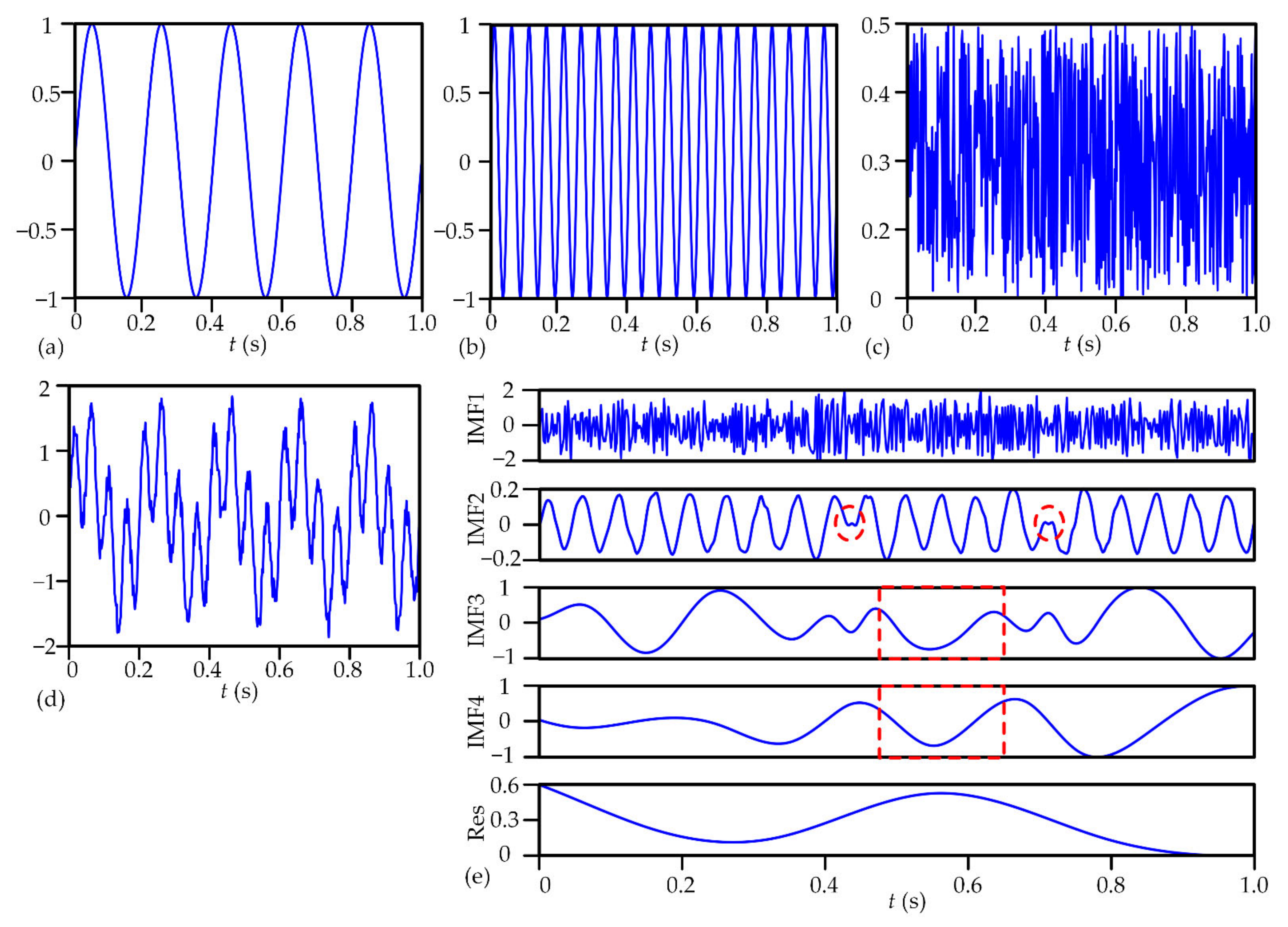
3.1. Signal Decomposition Method

(a)

Empirical mode decomposition (EMD)

EMD is a new time-frequency analysis method proposed by Huang and an adaptive time-frequency localization analysis method. Huang et al. [7] believe that any complex signal graph is composed of the most basic functions, which are IMF components based on the nature of the signal itself. Each IMF component needs to meet two basic conditions.

(1)

In the whole data sequence, the number of extreme points and the number of zero crossing must be equal, or the maximum difference can not be more than one.

(2)

For any point, the average value of the upper envelope and the lower envelope is zero.

The HHT method is an empirical method, and the empirical mode decomposition method may produce a mode mixing phenomenon and endpoint effect, which will directly affect the accuracy of EDM decomposition, resulting in a great difference between the experimental results and the actual ones. Only when the accuracy of modal decomposition is guaranteed, can the analysis results of the Hilbert Huang transform have real physical meaning.

In order to better explain the modal aliasing phenomenon, the Figure 3 is an example of signal synthesis and decomposition.

It can be seen from the EMD decomposition diagram that IMF1 corresponds to the white noise component, IMF2 corresponds to the high-frequency component, and IMF3 corresponds to the low-frequency component. It can be ideally considered that EMD decomposition gradually decomposes the frequency components in the original signal in the order from high frequency to low frequency, and each IMF represents the components of different frequencies in the original signal. IMF2 represents a high frequency sine wave with a frequency of 40Hz. However, in the decomposition diagram for IMF2, a waveform with a small characteristic time scale is visible. The waveform within the red circle is substantially different from the characteristic time scale of other positions. In the same band with two different peaks, there is a case of modal aliasing. In IMF3 and IMF4, the waveforms circled by the red boxes are very similar, and the appearance of similar waveforms in different components is also a manifestation of modal aliasing.

This example shows the superiority of EMD. This method can analyze the main components of the signal without specifying the basis function. Each frequency component of the original signal is decomposed step by step from high frequency to low frequency. At the same time, this reflects that EMD decomposition may produce redundant components and mode mixing, which directly affects the quality of EMD decomposition and determines the reliability of HHT decomposition results.

(b)

Ensemble EMD (EEMD)

In order to solve this problem, Wu Z and Huang N further proposed the Ensemble EMD (EEMD) method in 2009 [8]. This method added random white noise with different amplitudes to the original signal, and the added white noise sequences offset each other after integrated screening. The EEMD method can suppress modal confusion to some extent, while retaining the advantages of EMD. The key point of the EEMD method is to add different amplitudes of white noise to the original signal [8]. The specific process is as follows:

(c)

Complementary EEMD (CEEMD)

In 2010, Yeh et al. [9] proposed Complementary EEMD (CEEMD). The CEEMD method adds two opposite white noise signals to the original signal, and then conducts EMD decomposition respectively. The decomposition effect of this method is similar to that of EEMD, but it greatly reduces the reconstruction error caused by white noise. In order to understand the improved decomposition method more clearly, the following sections will introduce the decomposition method one by one. Based on the EEMD method, the CEEMD method adds white noise with opposite symbols to the target signal in pairs. The

Table 5. Advantages and disadvantages of three decomposition methods.

Method	Overview of Methods and Principles	Major Advantage	Major Defect
EMD	Decomposition Based on Signal Properties	EMD Decomposition without Presetting Basis Function	Aliasing phenomenon and endpoint effect
EEMD	The added white noise offsets each other after integrated screening	Suppress modal confusion to some extent; Improving the Quality of IMF Decomposition	Large amount of computation and decomposition depends on adding white noise amplitude and integration times
CEEMD	Add opposite white noise to the target signal in pairs	Reduced reconstruction error greatly; Better elimination of auxiliary residual noise	Large amount of calculation, adding white noise parameter selection is not appropriate, may appear false component

shows the main advantages and disadvantages of the four methods [9].

3.2. Evaluation System of Signal Decomposition Results

3.2.1. Completeness Evaluation

The completeness of signal decomposition, the reconstruction error, is defined as the difference between the original signal and the reconstructed signal of the sum of all IMF components. The completeness test is to reconstruct the signal of several IMF components after signal decomposition, and evaluate the completeness of the signal decomposition by checking the error between the reconstructed signal and the original signal [7].

Theoretically: the formula is an identity, the decomposition and reconstruction of the signal can be transformed into each other, and the completeness of the signal decomposition is theoretically satisfactory [7].

$$X\left(t\right)={\displaystyle \sum }_{i=1}^n{c}_i+r_n$$

(2)

From a numerical point of view: if the magnitude of the error between the calculated reconstructed signal and the original signal is very small, and the magnitude of the calculated error belongs to the rounding error of the computer accuracy, then the signal decomposition can be considered to meet the completeness [9].

3.2.2. Orthogonality Evaluation

The orthogonality of signal decomposition is an important indicator to evaluate the effect of signal decomposition. EMD decomposition is obtains a series of orthogonal narrowband components. The orthogonality of IMF components directly determines the decomposition efficiency of EMD. The higher the orthogonality, the less leakage between the components [7].

Huang et al. pointed out that a total orthogonality index IO is defined as [7]:

$$\mathrm{IO}={\displaystyle \sum }_{t=0}^T\left({\displaystyle \sum }_{j=1}^{n+1}{\displaystyle \sum }_{k=1}^{n+1}{C}_j\left(t\right)C_k\left(t\right)/X^2\left(t\right)\right)$$

(3)

Among them, T is the entire sampling duration of the signal.

3.3. Hilbert Transform

The basic idea of HHT is to decompose the original signal into several IMF components, and then a Hilbert transform is performed on each IMF to obtain the instantaneous frequency and instantaneous amplitude of each IMF component, so as to construct the time, frequency and energy distribution of the signal, namely the Hilbert spectrum [7]. Figure 4 shows the calculation flow of HHT method.

(1)

Taking time series data as an example, empirical mode decomposition algorithm:

$$X\left(t\right)={\displaystyle \sum }_{k=1}^n{c}_k\left(t\right)+r_n\left(t\right)$$

(4)

In the formula, $c_k\left(t\right)$ is the IMF; $r_n\left(t\right)$ is the residual function.

(2)

Hilbert time spectrum is obtained by Hilbert transform for each IMF component:

$$H\left(\omega ,t\right)=\mathrm{Re}{\displaystyle \sum }_{i=1}^n{a}_i\left(t\right)e^{j\int {\omega }_l\left(t\right)dt}$$

(5)

(3)

Hilbert marginal spectrum is obtained by the time integral of Hilbert spectrum:

$$h\left(\omega \right)={\displaystyle \underset{0}{\overset{T}{\int }}H\left(\omega ,t\right)\mathrm{d}t}$$

(6)

4. Experimental Results

In the model test, the fluctuating pressure signals at eight characteristic points on the bottom plate of the stilling basin with a negative step were measured under four flow energy ratios, with a fluctuating pressure sensor sampling time of 4 min. In the model test, due to the existence of various noise, the fluctuating pressure signal of the bottom plate of the stilling basin is often distorted, so it is necessary to use the signal processing method to restore the real signal of the fluctuating pressure. In this paper, the least squares method was used to remove the trend term, and the five-point cubic smoothing method was used to remove the noise. The fluctuating pressure signal of the bottom plate of the stilling basin was preprocessed. The instantaneous pressure measured by the fluctuating pressure sensor is equal to the superposition of the time-averaged pressure and the fluctuating value. Therefore, the fluctuating value is equal to the instantaneous value minus the time-averaged value.

4.1. Select Signal Decomposition Method

4.1.1. Completeness Check

Firstly, according to the completeness of signal decomposition, the best method was selected. The completeness of the test decomposition is to calculate the signal reconstruction error. Reconstruction error refers to the error between the reconstructed signal composed of IMF components and the original signal. The specific test method is to reconstruct several IMF components after signal decomposition, and evaluate the completeness of signal decomposition by calculating the error between reconstructed signal and original signal.

Theoretically, Formula (4) is an identity, and the decomposition and reconstruction of signals can be transformed into each other. The completeness of signal decomposition is theoretically satisfied. Numerically, by calculating the difference between the reconstructed data obtained by the sum of all IMF and the original data, if the magnitude of the calculation error is very small, the calculation error is considered as the round-off error of the computer accuracy. Then, it can be considered that the signal decomposition also satisfies the completeness from the perspective of numerical calculation.

Firstly, the P2 point on the bottom plate of the stilling basin with a negative step, TP4, is taken as an example when k = 0.0403. The fluctuating pressure value of the point is decomposed by EMD, EEMD and CEEMD methods, and the decomposition results of the three methods are obtained. At the same time, the reconstruction error of each method is calculated. According to the empirical formula calculation and repeated experiments, EEMD and CEEMD methods add noise amplitude is set to 0.01, and the amount of added noise is 200. The decomposition results and reconstruction errors of the three methods are as follows. Figure 5 shows the EMD decomposition results.

Figure 5 shows the original signal decomposed into IMF1, IMF2, IMF3, IMF4 and residual component.

Observing the Figure 5 of the P2 point on the bottom plate of the stilling basin TP4 at k = 0.0403, it can be seen that there are many modal aliasing phenomena, which may be caused by the interference of the noise signal in the experiment, or, may be caused by the limitations of the EMD method itself. Due to the accumulation of errors, the decomposition produces false components. The IMF component decomposed by the EMD method fails to describe accurately the real decomposition process of the original signal.

Figure 6 shows the EEMD decomposition results. It can be seen from the EEMD decomposition results that the EEMD method inhibits the modal confusion to a certain extent. This method effectively improves the decomposition quality of IMF, and the decomposed IMF can represent the real change process of the original signal.

Figure 6 shows the original signal decomposed into IMF1, IMF2, …, IMF12 and residual component Res.

Figure 7 shows the original signal decomposed into IMF1, IMF2, …, IMF12 and residual component RES.

Figure 7 shows the CEEMD decomposition results. The CEEMD method inhibits modal confusion to some extent. The residual component is reduced to 50% of EEMD method, which shows that the method can better eliminate the auxiliary residual noise and effectively improve the decomposition quality of IMF. The decomposed IMF components can represent the real process of the original signal.

Figure 8 shows the reconstruction error of EMD, EEMD and CEEMD. From the perspective of the reconstruction error of EMD decomposition, the reconstruction error of EMD decomposition is within ${10}^{-12}$. The magnitude of calculation error is very small. The amplitude of calculation error belongs to the round-off error of computer accuracy. From the perspective of numerical calculation, the signal decomposition satisfies the completeness. However, the EMD decomposition has obvious modal confusion, and the decomposition produces more false components. The decomposed IMF components cannot truly represent the original signal.

The EEMD decomposition results show that the EEMD method can suppress modal confusion to a certain extent, but some residual noise will be left in the decomposition process, which will eventually lead to large reconstruction error. The CEEMD decomposition results show that the CEEMD method adds the white noise with opposite symbols to the target signal in pairs on the basis of the EMD method, which effectively inhibits the mode mixing and greatly reduces the reconstruction error. The reconstruction error is about $5\times {10}^{-12}$, and the magnitude of calculation error is very small. It can be considered that the decomposition results of the CEEMD method meet the completeness. The reconstruction error of the CEEMD method and EMD decomposition belong to the same order of magnitude, indicating that the CEEMD method can better eliminate residual noise and significantly reduce the reconstruction error. The completeness of signal decomposition meets the requirements.

Based on the comprehensive decomposition results and reconstruction error calculation, this paper chose the CEEMD method decomposition results for the Hilbert transform.

4.1.2. Orthogonality Check

The orthogonality index of EMD is negative, indicating that the decomposition effect of this method is poor and the orthogonality of signal decomposition cannot meet the requirements [10]. When the white noise amplitude and integration times are the same, the orthogonality index of CEEMD method is greater than EEMD, indicating that the CEEMD method has the best decomposition effect and less signal leakage in the decomposition process.

Table 6. Comparison of indicators for signal decomposition.

Method	Add Noise Amplitude	Adding the Number of Noise	Index of Orthogonality
EMD	0	0	$-1.4\times {10}^{-3}$
EEMD	0.01	200	$2.6\times {10}^{-4}$
CEEMD	0.01	200	$6.8\times {10}^{-3}$

shows the index of orthogonality for signal decomposition.

The results of the completeness test and orthogonality test show that the reconstruction error of the CEEMD method is the smallest, and the orthogonality index is the largest. The calculation results show that the completeness and orthogonality of the CEEMD method are the best of the three methods. Therefore, the decomposition results from the CEEMD method are used for the Hilbert transform.

4.2. Hilbert Spectrum Analysis

In this paper, the CEEMD method decomposition results are selected for the Hilbert transform. The instantaneous frequency and instantaneous amplitude of the signal are obtained by a Hilbert transform of each IMF component, that is, the change law of the frequency domain of the signal with time [11]. The Figure 9 is the Hilbert spectrum of the IMF component at the bottom of the stilling basin x/L = 0.025 when k = 0.0403 for TP4 of the drop-sill stilling basin.

Figure 9 can intuitively reflect the fluctuation of the frequency of the fluctuating pressure signal of the bottom plate of the stilling basin with time. The Hilbert spectrum amplitude of each IMF component changes randomly with time. With the increase of order, the signal frequency band gradually narrows, and the Hilbert spectrum amplitude gradually decreases. The frequency band of the first decomposed component is relatively wide, and the amplitude is also large. After decomposition, the frequency band is narrow and the amplitude is low. It can be seen from the figure analysis that the lower the frequency is, the smaller the Hilbert spectrum amplitude is, and the lower the fluctuating pressure energy is. From the perspective of time and frequency resolution, the instantaneous frequency with practical physical significance can be obtained by decomposing the pulsating pressure signal based on the nature of the signal itself.

The Hilbert spectrum of each IMF component shows low frequency, especially in the IMF component after decomposition. According to the theory of turbulence mechanics, the low frequency component of the signal represents the large-scale turbulent vortex in the turbulence. Therefore, there are low frequency components with different bandwidth in the fluctuating pressure signal, and there are different scales of vortices in the turbulence. The random mixing of different scales of vortices leads to high turbulence in the water body. In this paper, the components of different bandwidths can be obtained by decomposing the fluctuating pressure signal, which can be understood as decomposing the turbulent water body into vortices of multiple scales, reflecting the vortex structure in the turbulence. At the same time, the vortex structures of different scales can be analyzed separately from the perspectives of time domain and frequency domain.

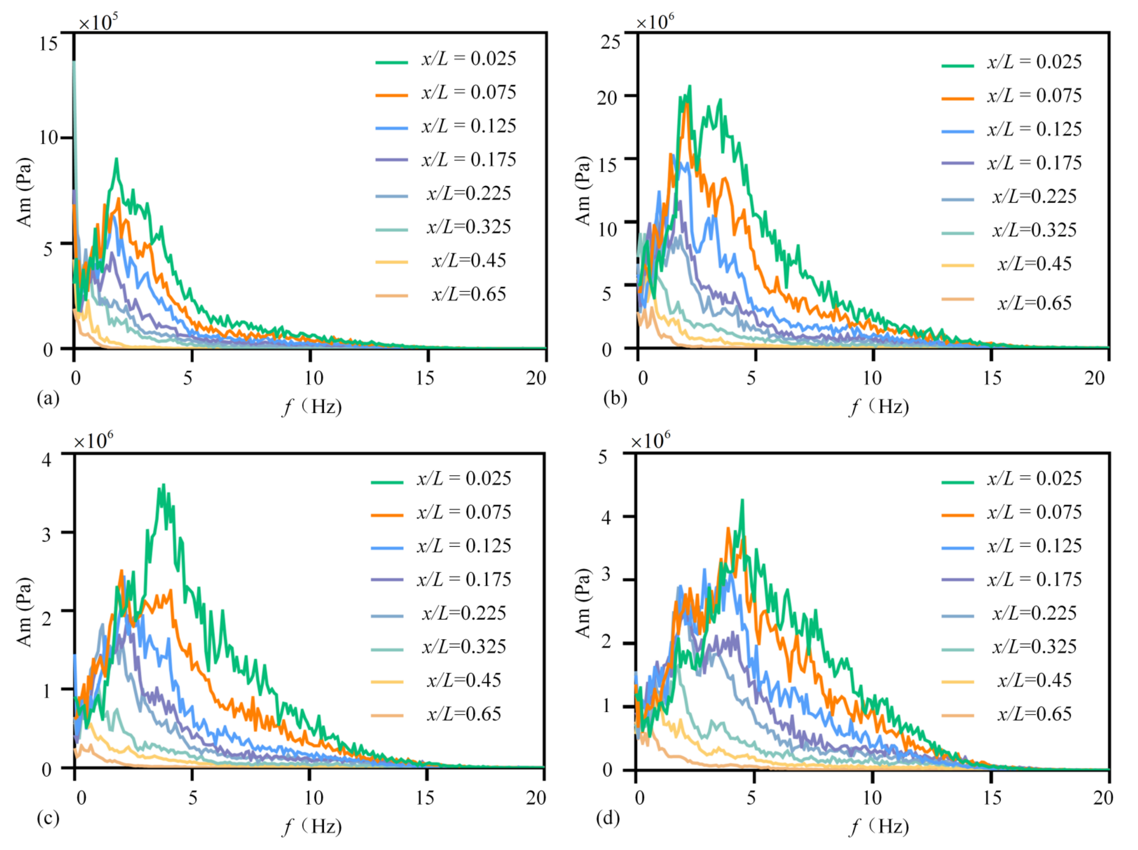
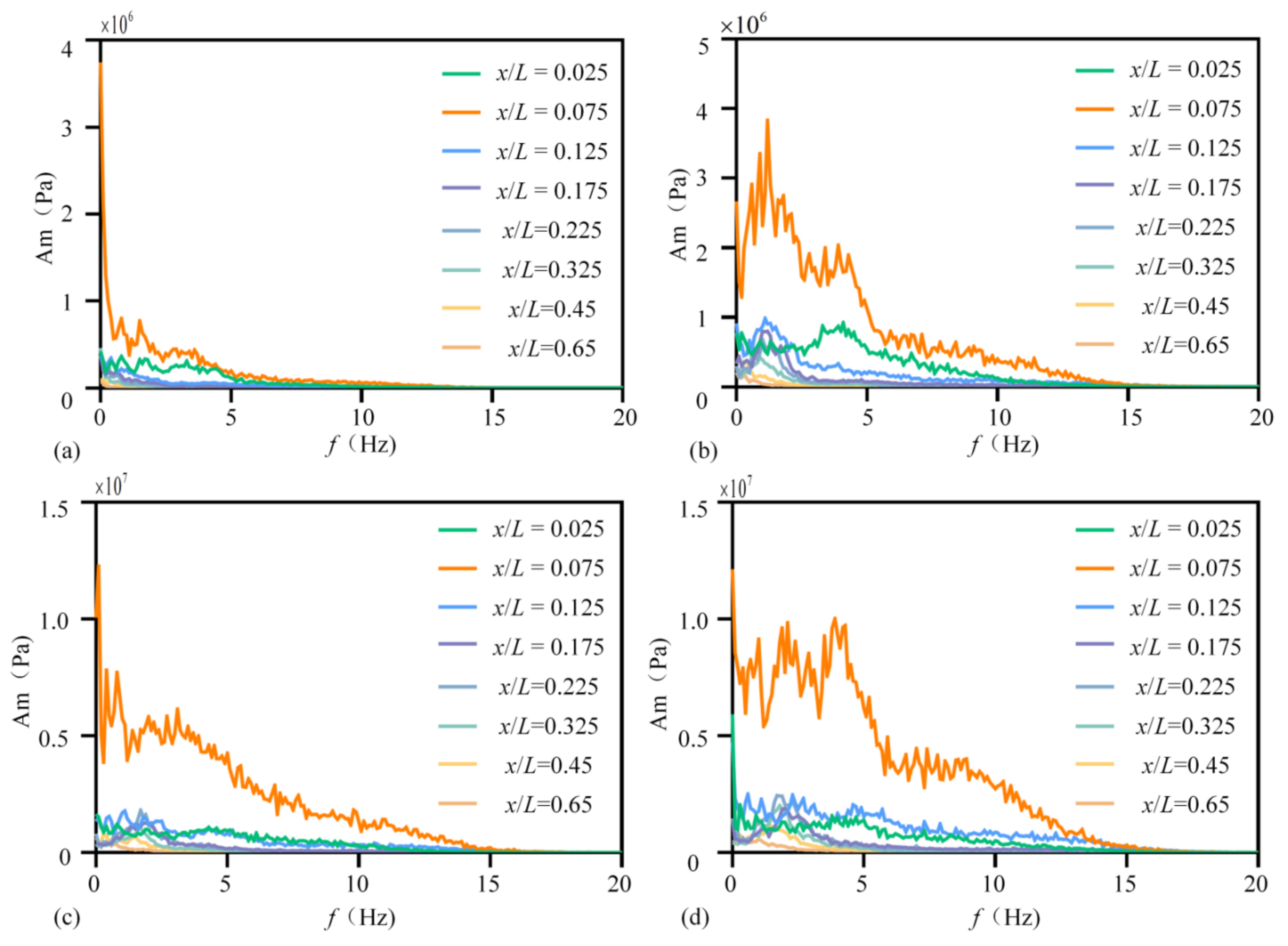
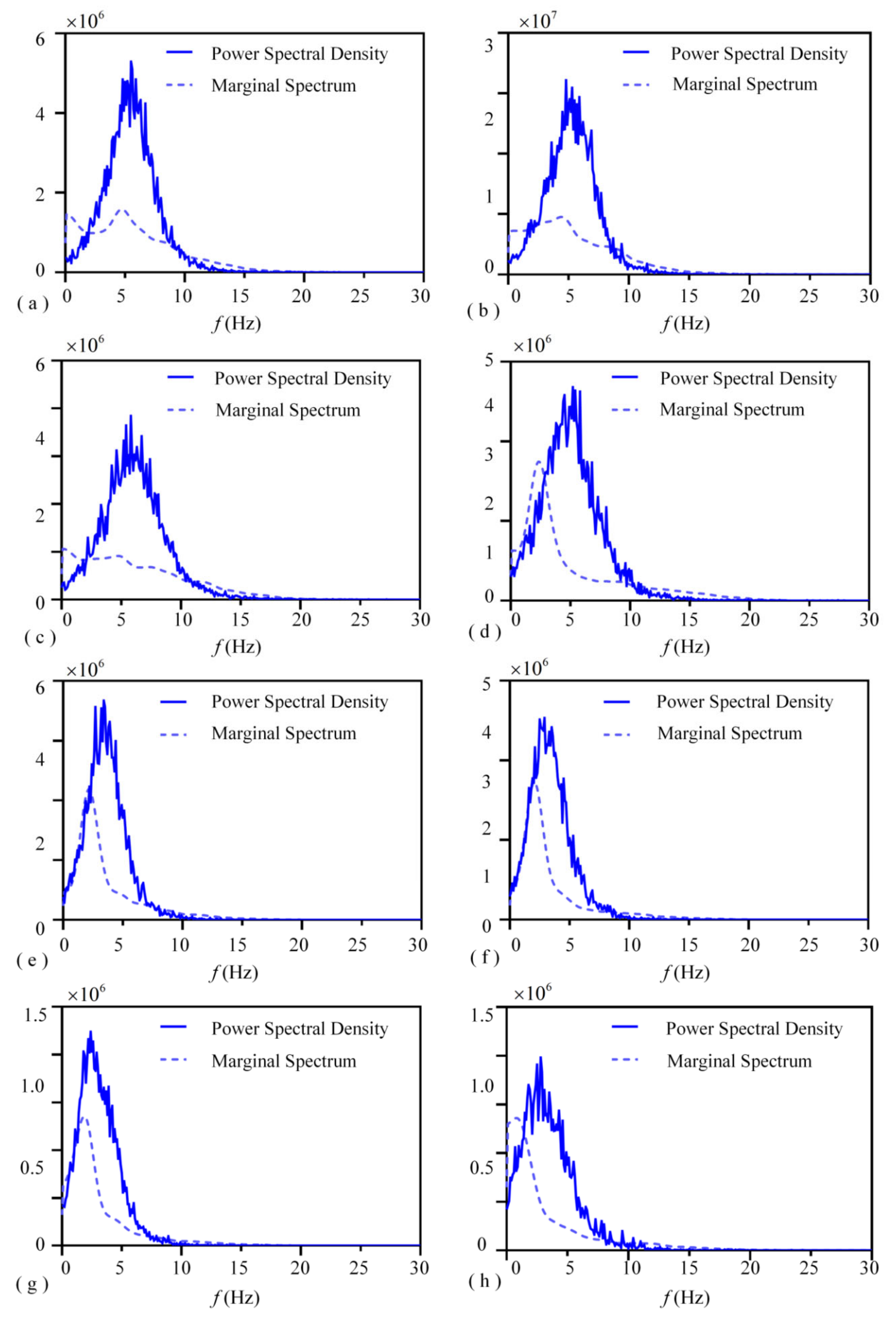
4.3. Hilbert Marginal Spectrum Analysis

The marginal spectrum is the change of signal amplitude in the whole frequency range, and also reflects the change rule of energy [12]. In order to analyze the energy variation law of each characteristic point in the bottom plate of the stilling basin, this paper calculates the marginal spectrum of TP0 and TP4 in the stilling basin with a negative step at different flow energy ratios.

Figure 10 shows the Hilbert marginal spectrum of fluctuating pressure at the characteristic point of TP0 bottom plate. Figure 11 shows advantage frequency and marginal spectrum amplitude. When k = 0.0134, the dominant frequency of the first part of the stilling basin is 2.0 Hz, and the dominant frequency of the middle and rear parts is close to 0. The marginal spectrum amplitude of each feature point increases sharply in the low-frequency region, and decreases rapidly in the low-frequency region. From the head to the tail of the stilling basin, the pulsating energy gradually decreases, reflecting the energy dissipation effect of the stilling basin.

When k = 0.0223, the dominant frequency of the stilling basin moves right relative to k = 0.0134, the dominant frequency band increases, and multiple peaks appear. The amplitude of the marginal spectrum increases significantly, and the pulsation energy increases. The marginal spectrum amplitude of each feature point increases sharply in the low frequency band and decreases sharply in the high frequency band. Along the axis of the bottom plate of the stilling basin, the dominant frequency and marginal spectral amplitude decrease.

When k = 0.0308, the dominant frequency of the stilling basin moves to the right relative to k = 0.0223, the dominant frequency band increases, and multiple peaks appear. The marginal spectrum amplitude of each feature point decreases along the path, and the marginal spectrum energy at the head of the stilling basin is greater than that at the tail of the stilling basin. The dominant frequency gradually decreases along the path, and the dominant frequency of each feature point is less than 4.0 Hz.

When k = 0.0403, the dominant frequency of each feature point of the stilling basin is less than 5.0 Hz. The dominant frequency of the head of the stilling basin is the largest, and gradually decreases along the bottom of the stilling basin. The amplitude of the marginal spectrum shows an increasing trend in the low frequency band and a decreasing trend in the high frequency band. The marginal spectrum energy at the head of the stilling basin is much larger than that at the rear of the stilling basin, and the marginal spectrum energy decreases gradually along the distance.

In the conventional stilling basin, the marginal spectrum amplitude of fluctuating pressure appears at the head of the stilling basin, and the marginal spectrum amplitude shows a trend of attenuation along the path. The marginal spectrum amplitude decays faster at the head of the stilling basin, and the attenuation speed of the marginal spectrum amplitude at the back of the stilling basin gradually slows down. There are multiple peaks in the marginal spectrum, namely multiple dominant frequencies. The first and second dominant frequencies are in the range of 1.0–5.0 Hz. In general, the marginal spectrum amplitude shows the characteristics of low frequency and large amplitude. The marginal spectrum energy decreases along the path, and the energy dissipation effect is good.

Figure 12 shows the Hilbert marginal spectrum of fluctuating pressure at the characteristic point of TP4 bottom plate. Figure 13 shows advantage frequency and marginal spectrum amplitude of TP4 bottom plate. From the marginal spectrum under different hydraulic conditions, it can be seen that the marginal spectrum amplitude at x/L = 0.075 is much larger than that at other locations, and the marginal spectrum energy is much larger than that at other locations. It can be seen from the dominant frequency table that under the same hydraulic conditions, the fluctuating pressure of the stilling basin with a negative step shows obvious low frequency.

When k = 0.0134, the dominant frequency of the bottom plate of the stilling basin with a negative step tends to 0. When k = 0.0223, the dominant frequency of the bottom plate of the stilling basin is within 1.2 Hz. When k = 0.0308, the dominant frequency of the stilling basin with a negative step floor is less than 1.5 Hz. When k = 0.0403, the dominant frequency of the stilling basin floor is less than 2.0 Hz. From the marginal spectrum amplitude table, it can be seen that under the same hydraulic conditions, the marginal spectrum amplitude of the fluctuating pressure at the bottom plate of the stilling basin with a negative step reaches the peak value near x/L = 0.075 and then decreases sharply, and finally tends to be stable. As k increases, the marginal spectral amplitude increases.

By comparing the marginal spectrum of the conventional stilling basin and the stilling basin with a negative step, it can be seen that the energy dissipation effect of the stilling basin is obviously better than that of the conventional stilling basin. Under the four hydraulic conditions, the marginal spectrum energy of the conventional stilling basin decreases gradually along the path, and the energy dissipation rate of the head of the stilling basin is slow. The energy dissipation effect of the stilling basin with a negative step is obvious. After the jet impingement zone, the marginal spectrum energy decreases significantly. After x/L = 0.075, the energy decreases rapidly and then tends to be stable. Therefore, it also shows that the energy dissipation effect of the stilling basin with a negative step is significant [13].

The HHT calculation results show that the jet impingement zone is near x/L = 0.075, and the dominant frequency of the jet impingement zone is very prominent. The marginal spectrum energy is also far greater than that of other positions, and most of the marginal spectrum energy is concentrated within 5.0 Hz; When x/L = 0.075, the proportion of high frequency band energy increases, and the dominant frequency band moves to high frequency. The whole integration of the marginal spectrum represents the energy of the flow pulsation at this point. From the marginal spectrum, it can be seen that the energy of the flow pulsation in the jet impingement zone in the stilling basin is far greater than that in other locations under different hydraulic conditions [14]. From the frequency domain, it is shown that the jet impingement zone in the stilling basin with a negative step is the region with the strongest pressure fluctuation [15]. Vortices at different scales are randomly mixed, and the water quality points have strong lateral movement, which makes the flow in the jet impingement zone highly turbulent, and the pressure fluctuation near this region very intense.

5. Discussion

5.1. Discussion on the Applicability of HHT Method

According to previous research, the variance of the fluctuating pressure signal can be called the average power of the fluctuating pressure signal, which reflects the energy of the signal. In order to facilitate the analysis of the energy characteristics of the fluctuating pressure signal, the variance of the signal in each frequency band is calculated. The variance of the IMF component of the characteristic point of the bottom plate of the stilling basin is statistically analyzed when the TP4 is k = 0.0403.

Table 7. Statistical table of signal variance decomposition (${\mathrm{Pa}}^2$ ).

IMF	x/L = 0.025	x/L = 0.075	x/L = 0.125	x/L = 0.175	x/L = 0.225	x/L = 0.325	x/L = 0.45	x/L = 0.65
IMF1	201,359.7	1,039,047.8	291,110.8	60,200.9	46,389.5	26,941.2	16,658.3	10,080.6
IMF2	131,046.4	905,789.8	215,922.7	79,423.8	125,754.5	84,511.2	43,321.4	13,802.9
IMF3	556,68.0	443,704.3	117,309.4	85,345.5	66,837.5	51,122.8	41,138.7	18,012.7
$⋮$	$⋮$	$⋮$	$⋮$	$⋮$	$⋮$	$⋮$	$⋮$	$⋮$
IMF13	11,405.1	5231.9	8943.7	927.0	3204.6	181.6	176.4	417.0
Sum	472,788.4	2,745,517.5	743,726.6	264,555.3	266,273.1	183,756.1	124,636.0	65,125.7
Original variance	456,207.8	2,794,908.8	765,561.3	279,251.3	261,882.2	198,237.3	135,588.3	70,413.6
Error (%)	3.6	−1.8	0.0	−0.1	0.0	−0.1	−0.1	−0.1

shows statistical table of signal variance decomposition.

It can be seen from the calculation results that the maximum error between the variance of the original signal and the sum of the variance of each component is 3.6%, the minimum error is 0%, and the error is approximately 0.1%. It can be considered that the variance before and after decomposition is approximately equal, and the error can be considered to be caused by calculation errors and other reasons, within the allowable range. The CEEMD method decomposes the signal, and the energy of the signal before and after decomposition is conserved. Therefore, it is considered that this decomposition method is suitable for the processing of fluctuating pressure signal of stilling basin floor.

According to previous studies, the conventional spectrum analysis method for studying fluctuating pressure signals is the fast Fourier transform method, which has the advantages of high efficiency, fast speed and reduced the calculation. In order to verify the rationality of the calculation results of the HHT method, the calculation results of HHT method are compared with those of fast Fourier transform. The TX4, k = 0.0403, the power spectral density map of each characteristic point of the stilling basin bottom plate, and the Hilbert marginal spectrum are compared and analyzed. Figure 14 shows the power spectrum density diagram and Hilbert marginal spectrum diagram of each feature point on the bottom of the stilling basin with a negative step.

When TX4, k = 0.0403, the fluctuating pressure signals of eight characteristic points on the bottom plate of the stilling basin with a negative step are processed by HHT method and FFT method respectively. The results show that the marginal spectrum obtained by the HHT method has higher resolution, more accurate local characteristics of the signal, and more clearly reflects the fluctuation characteristics of the marginal spectrum amplitude.

The marginal spectrum calculated according to the HHT method is consistent with the distribution law of the pulsating pressure power spectrum calculated by the Fourier transform. The marginal spectrum amplitude and the corresponding frequency when the power spectrum density amplitude reaches the maximum value are very similar, that is, the dominant frequencies calculated by the two methods are consistent.

The time-frequency resolution of the Hilbert marginal spectrum is higher than that of the Fourier spectrum. The power spectrum density obtained by fast Fourier transform can only represent the possibility of a certain frequency, and it is not a real frequency feature map. However, the marginal spectrum obtained by Hilbert-Huang transform is a real reflection of the vibration frequency distribution of the signal. When dealing with non-stationary and non-linear time series, the HHT method is more applicable in terms of calculation method. The fast Fourier transform is not suitable for dealing with non-linear and non-stationary signals. It is necessary to set assumptions in advance and select the basis function [16]. The HHT method is a method to obtain the time-frequency characteristics of the signal according to the characteristics of the signal itself. From the calculation results, the frequency resolution of the marginal spectrum calculated by the HHT method is higher, and the time-frequency-amplitude three-dimensional feature map can be obtained by combining the Hilbert spectrum, which is more conducive to capturing the instantaneous characteristics of the signal.

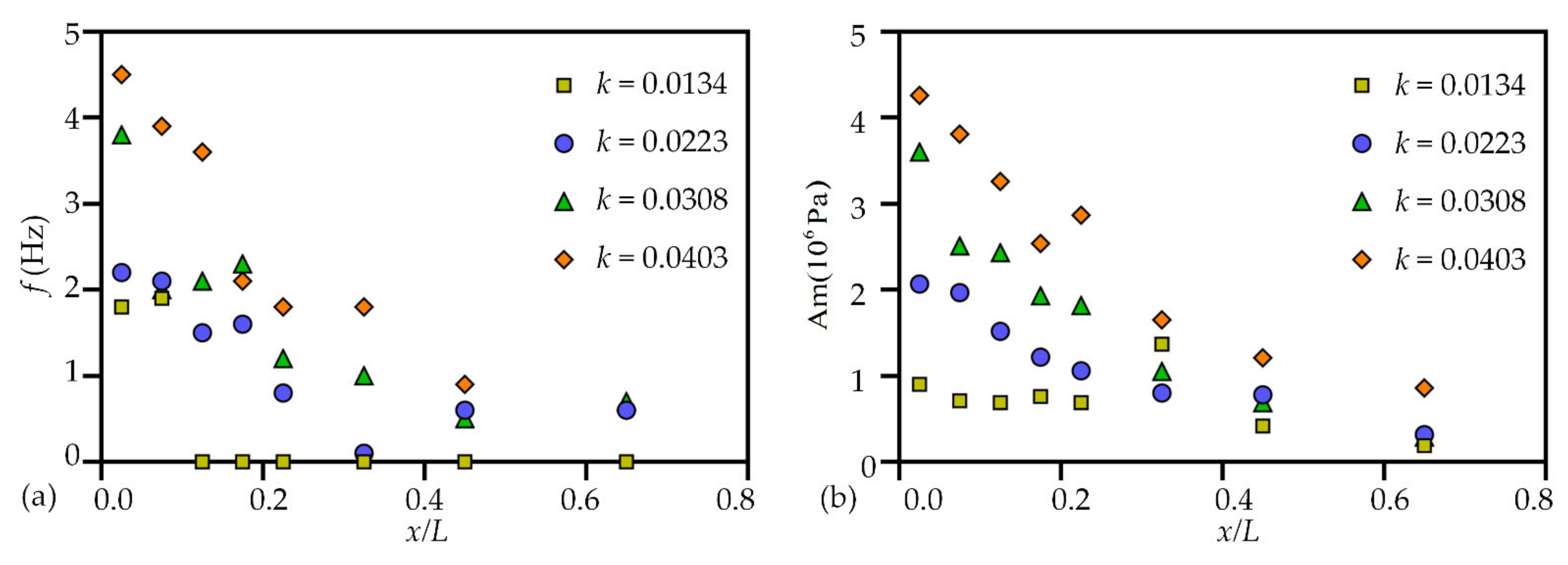
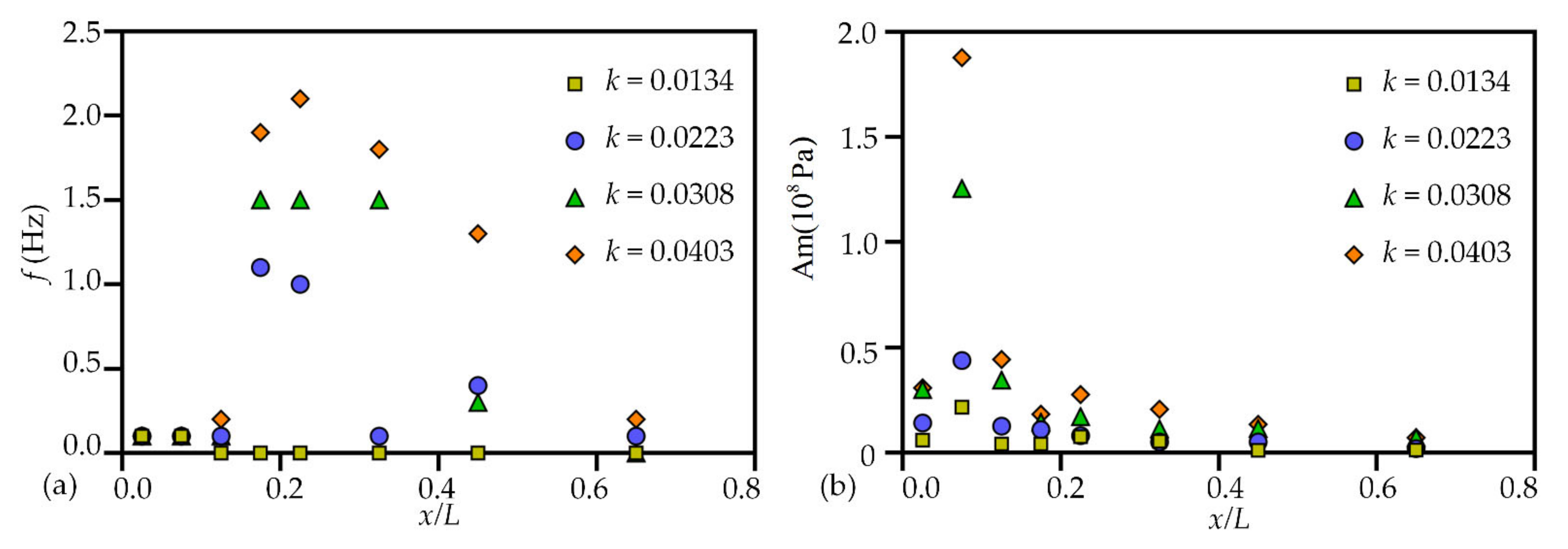
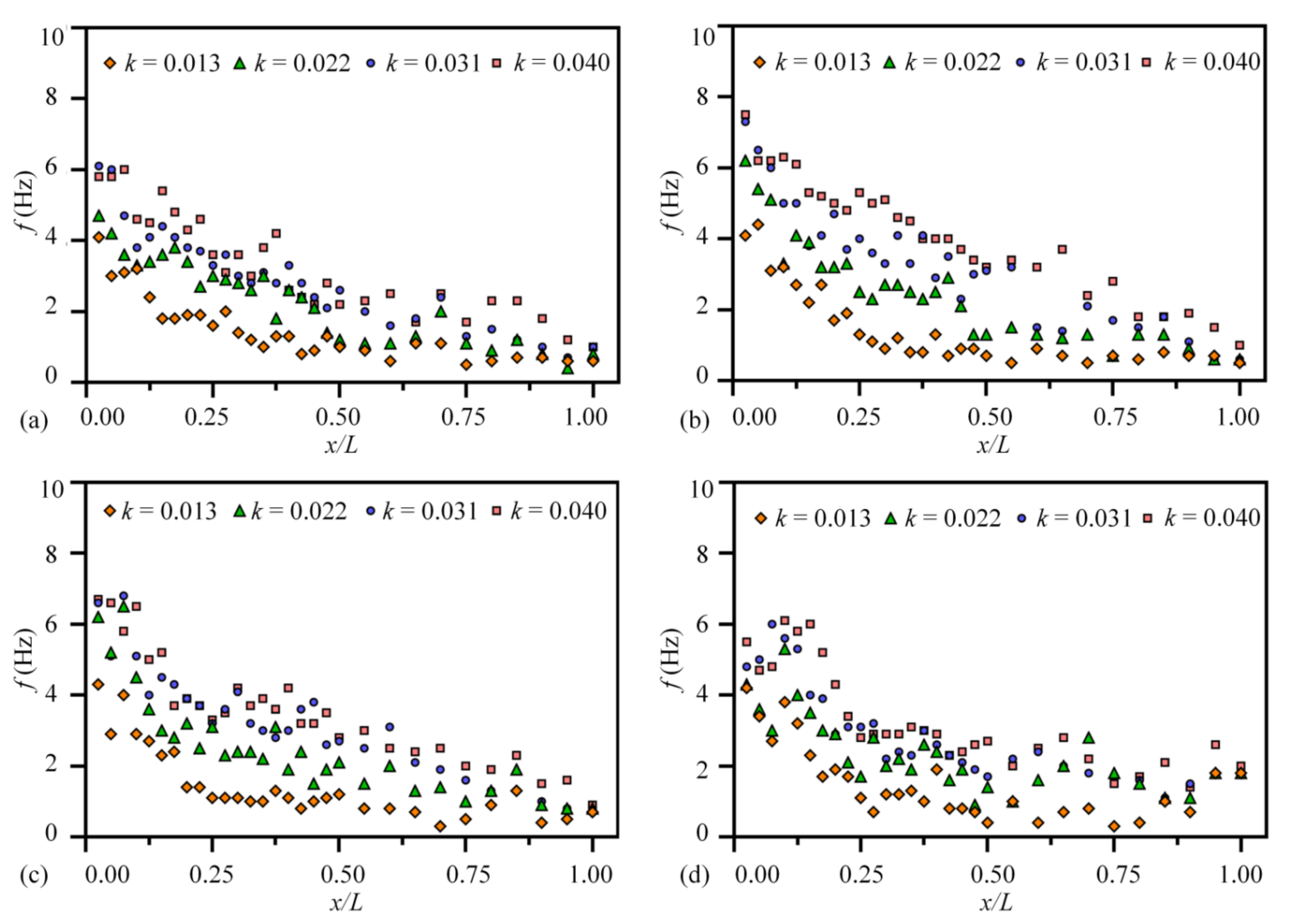
5.2. Distribution of Dominant Frequency of Different Body Types

In order to further study the distribution of dominant frequencies under different flow energy ratios, four types of stilling basin with a negative step were designed, and the number of characteristic points on the bottom of the stilling basin with a negative step was increased to 30 points. Under the four flow energy ratios, the relative distance of 30 characteristic points on the central axis of the bottom of the stilling pool is taken as the abscissa, and the dominant frequency is the ordinate. Different flow energies are compared with the dominant frequency of the fluctuating pressure on the bottom of the stilling basin with a negative step. Figure 15 shows the distribution of dominant frequencies along the way.

According to the experimental data, it can be seen that at different step-down heights and different flow energy ratios, the distribution law of the dominant frequency of the pulsating pressure of the bottom of the stilling basin with a negative step is similar, and the volatility of the dominant frequency decreases along the way, but has an overall decreasing trend. Under the four step-down heights, the dominant frequency is within 8.0 Hz, showing low frequency overall. The dominant frequency at the head of the stilling pool is larger, the dominant frequency at the middle and rear tends to be stable, and the dominant frequency is finally stabilized at about 1.0 Hz. According to turbulence mechanics, large-scale vortices in water flow cause low-frequency components of fluctuating pressure signals, and small-scale vortices cause high-frequency components. As a result, the vortex generated at the head of the stilling pool is mainly of small scale, and the vortex generated at the tail of the stilling pool is mainly of large scale.

6. Conclusions

This article used three methods to decompose the pulsating pressure signal, and a Hilbert transform was used to select the component with the best decomposition effect through the signal decomposition evaluation system. The Hilbert spectrum and Hilbert marginal spectrum of each feature point were calculated based on Hilbert transform, and the time-frequency characteristics and amplitude distribution of fluctuating pressure signals were obtained. The results of the HHT method and fast Fourier transform were compared, to explore the applicability of the HHT method in the signal processing of fluctuating pressure on the bottom plate of stilling basins with a negative step. The final important conclusions are as follows:

(1)

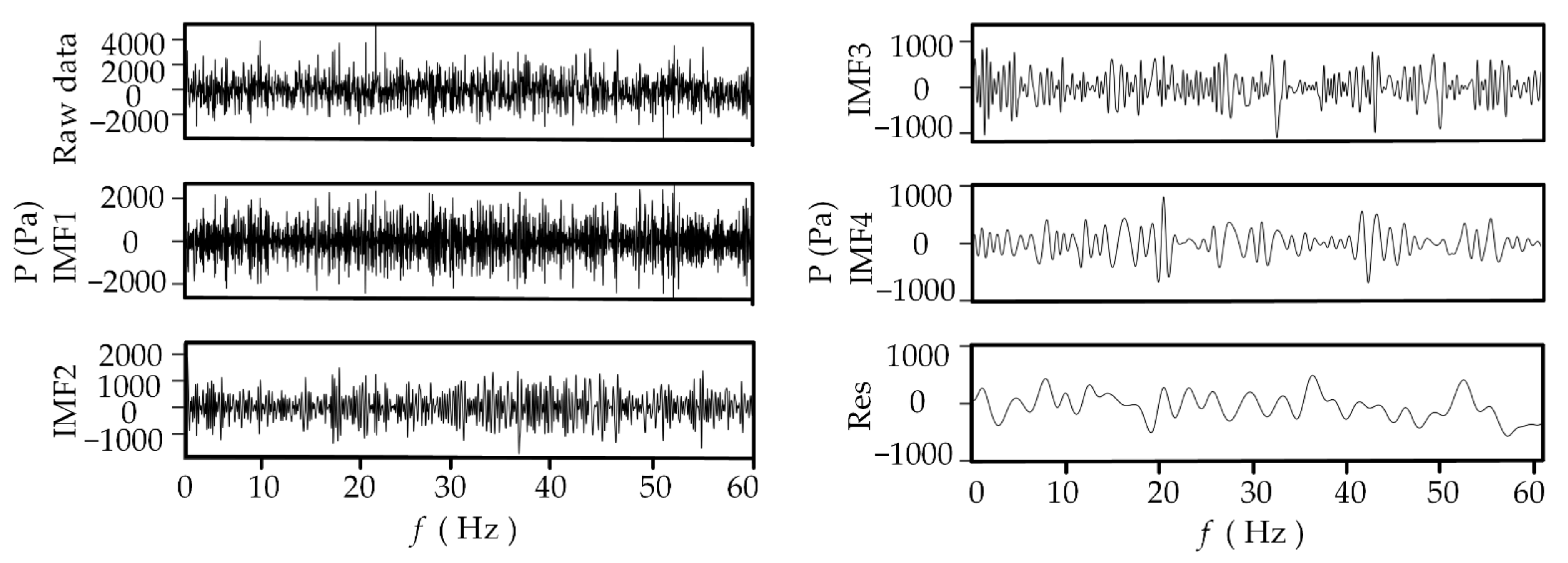
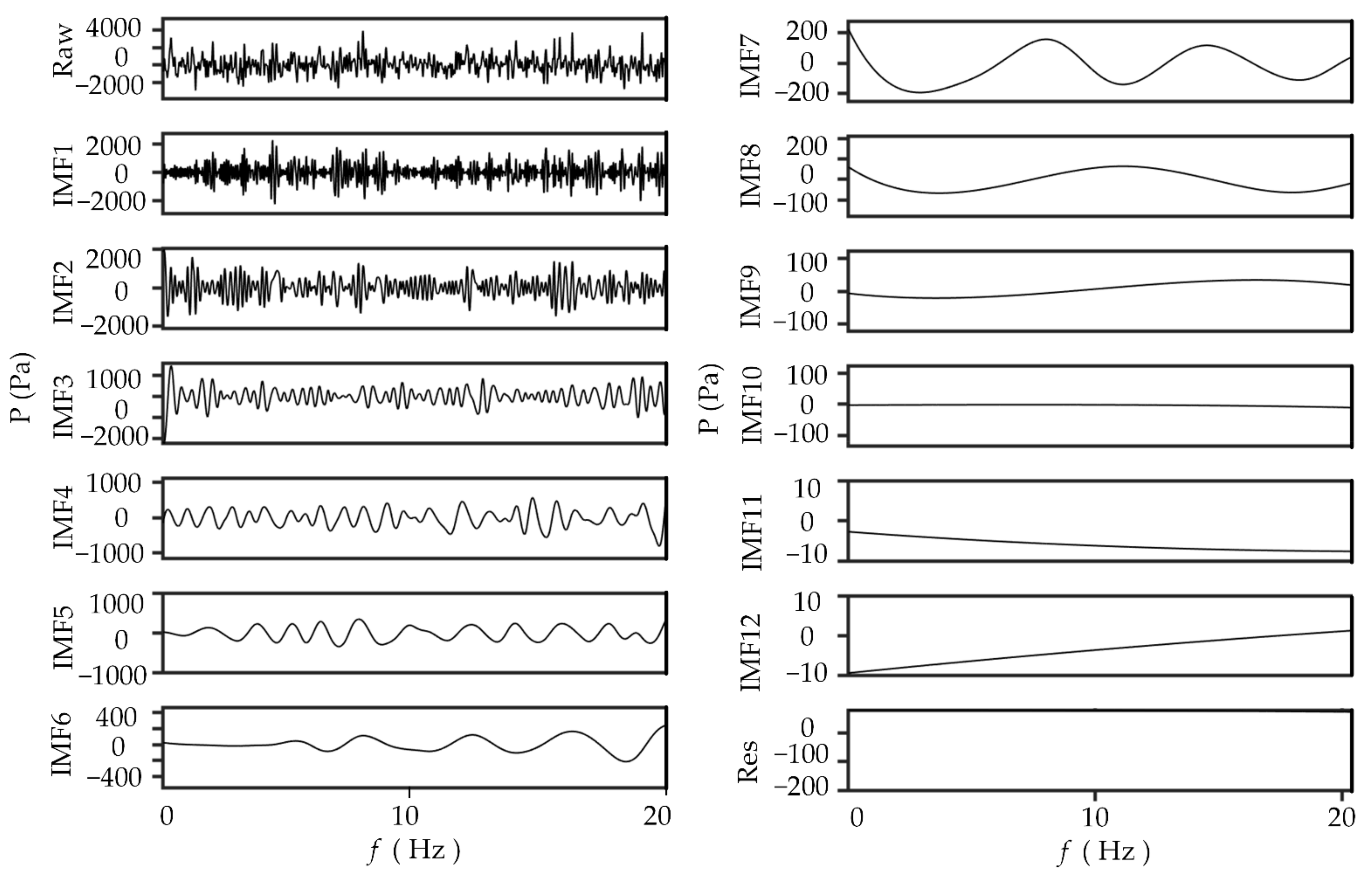
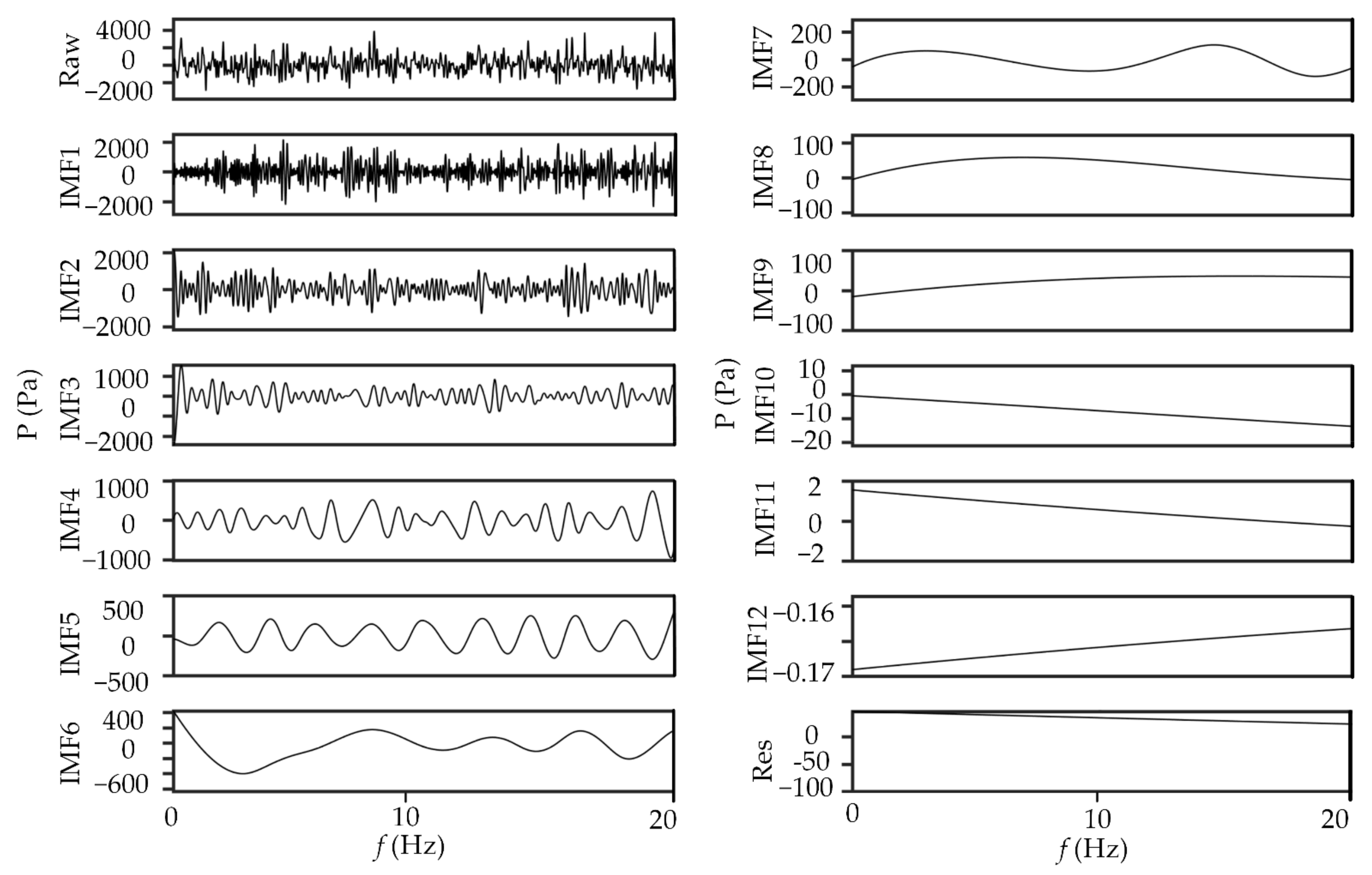
The decomposition results of fluctuating pressure signals show that the turbulence is composed of vortices with different scales, and this decomposition process reflects the vortex structure of turbulence. With an increase in IMF decomposition order, the signal frequency band becomes narrow and the pulsating pressure energy decreases. This shows that the energy contained in the first decomposed component is higher, which represents the high frequency and small scale vortex. When the decomposition of the component energy is low, this represents the low frequency, large scale vortex.

(2)

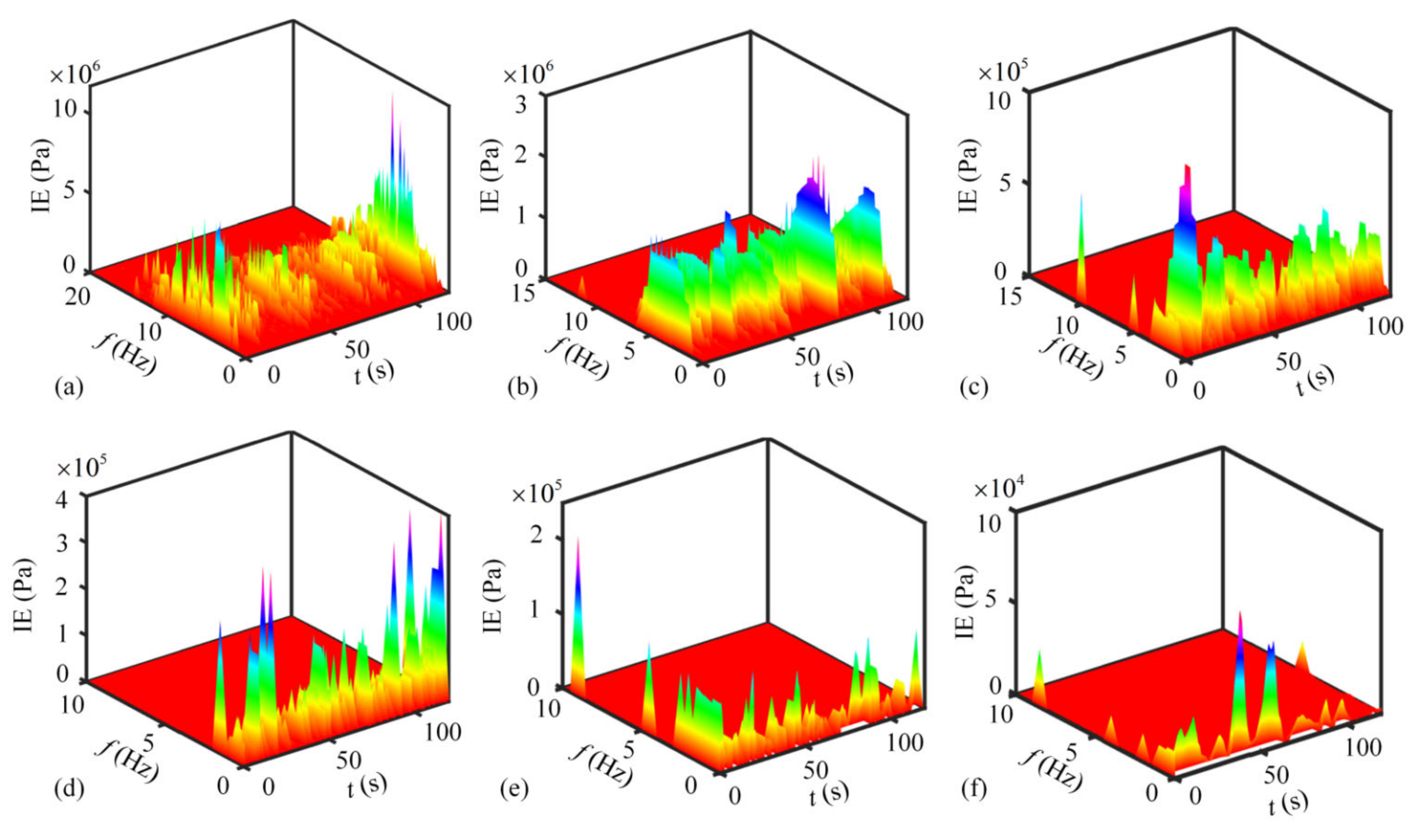
The jet impingement area of the stilling basin with a negative step is near x/L = 0.075, and the dominant frequency in this area is very prominent. The marginal spectral energy is also much larger than that in other locations, and most of the marginal spectral energy is concentrated within 5.0 Hz. After the jet impingement zone, the proportion of high frequency energy increases, and the dominant frequency band moves to high frequency. This indicates that near the jet impingement point, the signal energy is mainly concentrated in large-scale fluid vortices.

(3)

Under different drop heights and different flow energy ratios, the fluctuating pressure distribution of the bottom plate of the stilling basin with a negative step is similar. The dominant frequency of the head of the plunge pool is large, the dominant frequency of the middle and rear parts is stable, and the dominant frequency is finally stabilized at about 1.0 Hz. This shows that the fluctuating pressure of the bottom plate of the bucket stilling basin presents the characteristics of low frequency and large amplitude.

The decomposition results of the CEEMD method can not only effectively reduce the modal mixing phenomenon, but also meet the requirements of signal decomposition integrity and orthogonality. The energy conservation before and after signal decomposition and the calculation results of the HHT method and FFT method are consistent, which indicates that HHT technology is suitable for processing the fluctuating pressure signal of water flow. Hilbert-Huang transforms can not only transform the time domain analysis into frequency domain analysis, but also obtain the three-dimensional results of amplitude-frequency time, which broadens the dimension of the study on the characteristics of pulsating pressure.

References

1. Lu, Y.; Yin, J.; Yang, Z.; Wei, K.; Liu, Z. Numerical Study of Fluctuating Pressure on Stilling Basin Slab with Sudden Lateral Enlargement and Bottom Drop. Water 2021, 13, 238. [Google Scholar] [CrossRef]
2. Sun, S.K.; Liu, H.T.; Xia, Q.F.; Wang, X.S. Study on stilling basin with step-down floor for energy dissipation of hydraulic jump in high dams. J. Hydraul. Eng. 2005, 36, 1188–1193. [Google Scholar]
3. Fiorotto, V.; Rinaldo, A. Fluctuating Uplift and Lining Design in Spillway Stilling Basins. J. Hydraul. Eng. 1992, 118, 578–596. [Google Scholar] [CrossRef]
4. Deng, Z.; Guensch, G.R.; Richmond, M.C.; Weiland, M.A.; Carlson, T.J. Prototype measurements of pressure fluctuations in The Dalles Dam stilling basin. J. Hydraul. Res. 2010, 48, 822–823. [Google Scholar] [CrossRef]
5. Dai, C.; Kong, F.Y.; Dong, L. Study on Pressure Fluctuations of Unsteady Flow in a Circulating Water Pump. J. Comput. Theor. Nanosci. 2012, 9, 50–55. [Google Scholar] [CrossRef]
6. Zhang, X.; Wu, X.M. Time and Frequency Characteristics of Pressure Fluctuations during Subcooled Nucleate Flow Boiling. Heat Transf. Eng. 2018, 39, 642–653. [Google Scholar] [CrossRef]
7. Huang, N.E.; Shen, Z.; Long, S.R.; Wu, M.C.; Shih, H.H.; Zheng, Q.; Yen, N.C.; Tung, C.C.; Liu, H.H. The empirical mode decomposition and the Hilbert spectrum for nonlinear and non-stationary time series analysis. Proc. Math. Phys. Eng. Sci. 1998, 454, 903–995. [Google Scholar] [CrossRef]
8. Wu, Z.; Huang, N. Ensemble empirical mode decomposition: A noise-assisted data analysis method. Adv. Adapt. Data Anal. 2009, 1, 1–41. [Google Scholar] [CrossRef]
9. Yeh, J.R.; Shieh, J.S.; Huang, N.E. Complementary Ensemble Empirical Mode Decomposition: A Novel Noise Enhanced Data Analysis Method. Adv. Adapt. Data Anal. 2010, 2, 153–156. [Google Scholar] [CrossRef]
10. Laila, D.S.; Messina, A.R.; Pal, B.C. A Refined Hilbert–Huang Transform With Applications to Interarea Oscillation Monitoring. IEEE Trans. Power Syst. 2009, 24, 610–620. [Google Scholar] [CrossRef] [Green Version]
11. Petermichl, S. The sharp bound for the Hilbert transform on weighted Lebesgue spaces in terms of the classical A p characteristic. Am. J. Math. 2007, 129, 1355–1375. [Google Scholar] [CrossRef]
12. Fu, K.; Qu, J.; Chai, Y.; Zou, T. Hilbert marginal spectrum analysis for automatic seizure detection in EEG signals. Biomed. Signal Process. Control. 2015, 18, 179–185. [Google Scholar] [CrossRef]
13. Armenio, V.; Toscano, P.; Fiorotto, V. On the effects of a negative step in pressure fluctuations at the bottom of a hydraulic jump. J. Hydraul. Res. 2000, 38, 359–368. [Google Scholar] [CrossRef]
14. Yang, K.; Pan, Z.; Ye, P.; Shi, J.; Meng, J. A fast Fourier transform based method to estimate frequency response mismatches in time interleaved systems. Rev. Sci. Instrum. 2021, 92, 054709. [Google Scholar] [CrossRef] [PubMed]
15. Toso, J.W.; Bowers, C.E. Extreme pressures in hydraulic-jump stilling basins. J. Hydraul. Eng. 1988, 114, 829–843. [Google Scholar] [CrossRef]
16. Mokry, M.; Ohman, L.H. Application of the fast Fourier transform to two-dimensional wind tunnel wall interference. J. Aircr. 2012, 17, 402–408. [Google Scholar] [CrossRef]
Figure 1. Chart of stilling basin.
Water 13 02673 g001
Figure 2. Experiment setup.
Water 13 02673 g002
Figure 3. EMD decomposition case (unit: Pa). (a) Low-frequency sine wave with a frequency of 10 Hz; (b) A high-frequency sine wave with a frequency of 40 Hz, and (c) White noise with an amplitude of 0.5. The three waveforms are superimposed to obtain (d). (e) Shows IMF1, IMF2, IMF3, IMF4 and the residual component.
Water 13 02673 g003
Figure 4. Signal processing flow chart using HHT method.
Water 13 02673 g004
Figure 5. EMD decomposition results.
Water 13 02673 g005
Figure 6. EEMD decomposition results.
Water 13 02673 g006
Figure 7. CEEMD decomposition results.
Water 13 02673 g007
Figure 8. The reconstruction error of EMD, EEMD and CEEMD from top to bottom.
Water 13 02673 g008
Figure 9. Hilbert spectrum of IMF component at bottom plate x/L = 0.025 for TP4 at k = 0.0403. (a) The Hilbert spectrum of IMF 1; (b) The Hilbert spectrum of IMF 2; (c) The Hilbert spectrum of IMF 3; (d) The Hilbert spectrum of IMF 4; (e) The Hilbert spectrum of IMF 5; (f) The Hilbert spectrum of IMF 6.
Water 13 02673 g009
Figure 10. (a) k = 0.0134; (b) k = 0.0223; (c) k = 0.0308; (d) k = 0.0403, the Hilbert marginal spectrum of fluctuating pressure at the characteristic point of TP0 (Conventional stilling basin) bottom plate.
Water 13 02673 g010
Figure 11. (a) Advantage frequency table shows that k = 0.0134; k = 0.0223; k = 0.0308; k = 0.0403, the main frequency of the characteristic points of the bottom of the stilling pool; (b) Marginal spectrum amplitude table shows the marginal spectral amplitude of the characteristic points on the bottom of the stilling pool when k = 0.0134; k = 0.0223; k = 0.0308; k = 0.0403.
Water 13 02673 g011
Figure 12. (a) k = 0.0134; (b) k = 0.0223; (c) k = 0.0308; (d) k = 0.0403, the Hilbert marginal spectrum of fluctuating pressure at the characteristic point of TP4 bottom plate.
Water 13 02673 g012
Figure 13. (a) Advantage frequency table shows that k = 0.0134; k = 0.0223; k = 0.0308; k = 0.0403, the main frequency of the characteristic points of the bottom of the stilling pool; (b) Marginal spectrum amplitude table shows the marginal spectral amplitude of the characteristic points on the bottom of the stilling pool when k = 0.0134; k = 0.0223; k = 0.0308; k = 0.0403.
Water 13 02673 g013
Figure 14. The stilling basin with a negative step marked TX4, when k = 0.0403, power spectrum density diagram and Hilbert marginal spectrum diagram of each feature point on the bottom of the stilling basin with a negative step. (a) x/L = 0.025; (b) x/L = 0.075; (c) x/L = 0.125; (d) x/L = 0.175; (e) x/L = 0.225; (f) x/L = 0.325; (g) x/L = 0.45; (h) x/L = 0.65.
Water 13 02673 g014
Figure 15. (a) TP1, (b) TP2, (c) TP3, (d) TP4 under different flow energy ratio, the distribution of dominant frequencies along the way.
Water 13 02673 g015