Modelling Debris Flow Runout: A Case Study on the Mesilau Watershed, Kundasang, Sabah

Abstract

Debris flows are among the fatal geological hazards in Malaysia, with 23 incidents recorded in the last two decades. To date, very few studies have been carried out to understand the debris flow processes, causes, and runouts nationwide. This study simulated the debris flow at the Mesilau watershed of Kundasang Sabah caused by the prolonged rainfall after the 2015 Ranau earthquake. Several interrelated processing platforms, such as ArcGIS, HEC-HMS, and HyperKANAKO, were used to extract the parameters, model the debris flow, and perform a sensitivity analysis to achieve the best-fit debris flow runout. The debris flow travelled at least 18.6 km to the Liwagu Dam. The best-fit runout suggested that the average velocity was 12.5 m/s and the lead time to arrive at the Mesilau village was 4.5 min. This high debris flow velocity was probably due to the high-water content from the watershed baseflow with a discharge rate of 563.8 m³/s. The flow depth and depositional thickness were both lower than 5.0 m. This study could provide crucial inputs for designing an early warning system, improving risk communication, and strengthening the local disaster risk reduction and resilience strategy in a tectonically active area in Malaysia.

1. Introduction

Debris flows are among the disastrous geological hazards that occur in both developed and developing countries. This sediment-related disaster strikes quickly without warning, and results in severe consequences, including human and economic losses [1]. In 2021, a number of deaths due to debris flow alone were reported: debris flow in Uttarakhand, India (February 2021), which killed more than 200 people [2]; debris flow (mudslide) in Atami, Japan (July 2021), which killed at least three people, and 80 people remained missing [3]; and debris flow in Gunung Jerai, Kedah, Malaysia (August 2021), which wiped out at least six people with two victims still missing [4,5]. In Malaysia, approximately 23 debris flow incidents were recorded nationwide between 1995 and 2015 (

Table 1. Records of debris flows in Malaysia from 1995 to 2015.

No.	Date	Location	Triggering	Fatalities
1	30 June 1995	Km 38.6 Kuala Lumpur–Karak Highway, Genting Sempah, Selangor	Rainfall	20
2	29 August 1996	Kg. Orang Asli, Pos Dipang, Kampar, Perak	Rainfall	44
3	26 December 1996	Keningau, Sabah	Typhoon	302
4	January 2000	Cameron Highland, Pahang	Rainfall	6
5	22 September 2001	Chinchin Village, Gombak, Selangor	Rainfall	1
6	28 December 2001	Channelized Pulai river, Gunung Pulai, Johor	Rainfall	5
7	28 January 2002	Ruan Changkul, Simunjan, Sarawak	Rainfall	16
8	November 2002	Hulu Kelang, outskirt of Kuala Lumpur City	Rainfall	8
9	10 November 2003	Section 23.3 to 24.10 Kuala Kubu Baru, Selangor	Rainfall	0
10	2 November 2004	Km 52.4 Kuala Lumpur–Karak highway, Lentang	Rainfall	0
11	10 November 2004	Km 302 North South Expressway, G. Tempurung, Perak	Rainfall	0
12	November 2004	Taman Harmonis, Gombak, Selangor	Rainfall	1
13	12 April 2005	Km 33 Simpang Pulai, Cameron Highland, Pahang	Rainfall	0
14	15 November 2007	Km 4 to 5 Gap, Fraser’s Hill Road, Pahang	Rainfall	0
15	January 2008	Channel of Fraser Hill’s	Rainfall	0
16	3 January 2009	Section 62.4, Lojing Gua Musang Road, Kelantan	Rainfall	0
17	7 August 2011	Kampung Orang Asli Sungai Ruil, Cameron Highlands, Pahang	Rainfall	7
18	23 October 2013	Bertam valley, Cameron Highland	Rainfall	1
19	5 November 2014	Km 28, Jalan Tamparuli, Ranau, Sabah	Rainfall	0
20	11 Jane 2015	Channel of Fraser Hill’s	Rainfall	0
21	18 May 2015	Km 38.80, Jalan Penampang Tambunan Dongongan, Sabah	Rainfall	0
22	15 June 2015	Channelized Mesilau river, Kundasang, Sabah	Earthquake and rainfall	0
23	August 2015	Channelized Kedamaian, and Panataran river, Kota Belud, Sabah	Earthquake and rainfall	0

Sources: [7,8,9,10,11,12,13,14,15,16,17,18,19,20,21,22,23,24,25,26,27,28].

). These events were mostly induced by rainfall and very few were triggered by the cascading earthquake. Incidentally, Malaysia’s geographic location near the equator with a tropical climate receives an abundant annual rainfall, i.e., an average of 2400 mm [6]. In Sabah, the vicinity of Mount Kinabalu, the first UNESCO World Heritage Site in Malaysia has recorded two recent debris flows at the Mesilau watershed of Kundasang (the southeast flank of Mount Kinabalu) and the Kedamaian watershed of Kota Belud (the northwest flank of Mount Kinabalu), respectively [7,8].

The most fatal of debris flow in Malaysia occurred in 1996 at Keningau, Sabah, which killed 302 people and caused an economic loss of 458.9 million RM [23,25]. The debris flow was induced by Typhoon Gregg; it remains the deadliest geological disaster in the history of Malaysia. The first earthquake-induced debris flow in Malaysia happened in 2015 at the Mesilau watershed of Kundasang, Sabah, after prolonged post-earthquake rainfall. Although the debris flow recorded no fatality along the channelised river, it caused a significant socioeconomic impact and indirect economic losses [8,29,30].

The concept of debris flow initiation at the Mesilau watershed was adapted from the debris flow after the Gorkha earthquake of Nepal in 2015 [31]. After the earthquake, two forms of hazards, known as the primary and secondary hazards, were initiated [31]. The primary hazard encompasses the direct geological failures from the earthquake (i.e., rock avalanches, rock falls, and landslides), and the secondary hazard refers to the reactivated or remobilised landslides dam from the earthquake, for example, debris flows.

Incidentally, the initiation of debris flow of the Gorkha earthquake could also adequately describe the debris flow after the Ranau earthquake at the Mesilau watershed (Figure 1). The primary hazard was seen at the foot slope of Mount Kinabalu, where the earthquake induced many landslides, forming a temporary landslide dam, while the secondary hazard, known as debris flow, occurred along the channelised Mesilau river (Figure 1, the yellow polygon). Figure 2 shows the evidence of accumulated boulders along the channelised river after the debris flow.

The debris flow in the channelised Mesilau river was mainly induced by prolonged rainfall ten days after the 6.0 Mw Ranau earthquake on 5 June 2015 (Figure 3) with a series of aftershocks. Frequent rains were recorded for seven days with a cumulative rainfall of 66.3 mm and the highest rainfall intensity of 14.2 mm/h on 15 June 2015, which triggered the event. Chronologically, the extensive ground shaking from the main earthquake triggered many shallow and deep-seated landslides within the vicinity of Mount Kinabalu on 5 June 2015 and partially accumulated the debris and sediment as the temporary landslide dam [7]. The subsequent prolonged rainfall further reduced the stability of the landslide dam and reactivated the landslide dam as debris flow. Several debris flows impacted the channelised river and the village area, as reported by [8].

Several studies have been conducted to investigate the earthquake at Kundasang [7], which have focused mainly on the causes and impacts of the earthquake [8], landslide inventory [32,33], landslide susceptibility [34], landslide hazard and risk [35], land cover assessment [36], and business continuity plan [30]. However, little is known about the debris flow travelling along the channelised Mesilau river from the upstream to the downstream areas.

Debris flow modelling has become one of the effective methods to understand the debris flow processes [37]. The modelling of debris flow allows the simulation of past events, prediction of future events, and simulation of an area without historical evidence [38]. Therefore, the simulation results can contribute to the analysis of potential hazard scenarios and suitable planning for debris flow risk reduction strategies [39,40]. Generally, three methods for debris flow modelling are available which include physical modelling, empirical modelling, and dynamic modelling [41]. The differences between these methods are that physical modelling is conducted based on the field observation and supported by the controlled laboratory experiment; whilst the empirical modelling is performed based on the well-documented observation and, usually, it is practical to estimate the travel distance without considering the rheology of debris flow [42]. In addition, dynamic modelling is performed by using the numerical methods applying the momentum and energy conservation law [43]. Recently, a variety of debris flow simulation models exist globally, such as TRENT2D [44], AschFLow [45], HyperKANAKO [46], and RAMMS:Debris Flow [47,48]. Each model is distinguished by its applicability, price, parameters, and algorithms within the model [38].

This study examined the debris flow runout processes via simulation using HyperKANAKO and reconstruction of a past debris flow event. This study encompassed the preparation of the base model, extraction of the rainfall-runoff model, and model calibration for generating the best-fit debris flow runout via several interrelated processing platforms. A series of field investigations and interviews with the local community was also conducted to validate the runout results. The simulated result could provide important insight for improving the management of hazards and risks in this tectonically active area.

2. Materials and Methods

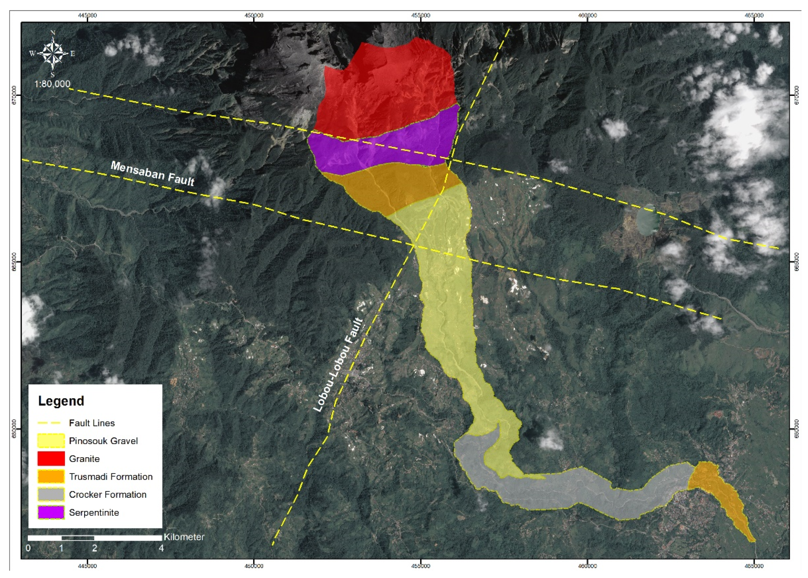
2.1. Study Area

The selected study area is an undulating terrain located at the southeast flank of Mount Kinabalu, Kundasang with altitudes ranging from 578 to 2384 m [7]. Figure 4 shows the Mesilau watershed, ranging from the upstream area in the mountain to the downstream area in the Ranau town (the irregular yellow boundary), while the source area of debris flows is located in the eastern plateau of Mount Kinabalu (the red polygon). The latitudes of the study area range between 06°05′02.0″ and 05°57′34.6″, while the longitudes encompass 116°32′53.3″ and 116°41′01.6″.

There are three settlements within the study area (green polygons), i.e., the Mesilau village, Naradau village, and Ranau town. Unlike the other two settlements, the Mesilau village has been exposed to many geological hazards and associated risks due to its proximity to the foot slope of the mountain, two main rivers, and tourist areas with many attractive infrastructures. These infrastructures include Desa Dairy Farm, Mesilau Golf Club, Strawberry Farm Mesilau, Mesilau Cat’s village, Mesilau Nature Resort, homestays, Maragang hill, and Sososdikon hill [7]. The area is also widely known as one of the primary agriculture production zones in Sabah, due to its climate, topography, and tourism activities in the vicinity of Mount Kinabalu.

Geologically, the study area is mainly dominated by five lithologies, i.e., Serpentinite, the Crocker formation, the Trusmadi formation, Granite, and the Pinousok gravel [49,50,51,52]. The Crocker formation consisted of strongly folded and faulted sandstone, siltstone, red and grey shale, mudstone, and argillite; the Trusmadi formation can be described as strongly folded and faulted grey and dark grey argillite, slate, siltstone and sandstone with volcanic; and the Pinousok gravel is characterized by its poorly unconsolidated gravel up to boulder sizes in a sandy to clayey matrix [49,50,51,52,53]. Typically, these lithologies comprised mostly weathered materials [54]. Figure 5 shows the five lithologies within the watershed. The source area at the foot slope of Mount Kinabalu is comprised of the granitic rock and Serpentinite, while the transportation and deposition area is comprised of Pinousok gravel, Crocker formation, and Trusmadi formation. There are two major prominent and active faults in the study area: the Lobou-Lobou fault, a left-lateral strike faulting N20E and the Mensaban fault trending northwest-southeast [55]. The associated fault during the 2015 Ranau earthquake was due to the normal slip of the Lobou-Lobou fault, with the epicentre located at the highland of Kundasang town and a shallow depth of 10 km beneath Mount Kinabalu [8]. Historically, the Ranau district recorded three earthquakes exceeding 5.0 Mw [7,8], i.e., in 1966 (Mw 5.3), 1991 (Mw 5.2), and 2015 (Mw 6.0), with approximate return periods of every 24 to 25 years [7]. Evidence of weak geological materials and earthquake studies have categorised this area as high risk to geological hazards and the associated risks [54,56,57].

2.2. Datasets

This study employed three main datasets, i.e., the orthophoto, Digital Terrain Model (DTM), and rainfall dataset (

Table 2. The types of datasets used for this study.

Type of Dataset	Source	Resolution/Record	Date
Orthophoto	LiDAR	0.07 m	2016
DTM (before debris flow)	IfSAR	5.0 m	2008
DTM (after debris flow)	LiDAR	0.25 m	2016
Rainfall	Rain-gauge	Hourly, mm	June 2015

). Additionally, the Light Detection and Ranging (LiDAR) point-cloud dataset was obtained from the Department of Mineral and Geoscience Malaysia (JMG Malaysia); it was acquired a year after the earthquake disaster under the Slope Hazard and Risk Mapping (PBRC) project. The LiDAR acquisitions (i.e., orthophoto and DTM) were conducted through airborne laser scanning (ALS) with the combined systems of Laser Scanner 6800-400, IMU-Ilf Inertial Measurement Unit, Trimble R7 GPS Receiver, DigiCAM H60, DigiCAM Lens Cone HC 3,5/50-11, Clear-Protection-Filter, 77 mm, LiteMapper system mount, LiteMapper Data Recorder 680, and AEROcontrol Sensor Management Unit [58]. The Interferometric Synthetic Aperture Radar (IfSAR) dataset was acquired from the Intermap STAR Technologies^®’ proprietary X-Band IfSAR, and the hourly rainfall records were retrieved from the Malaysian Meteorological Department (MMD). The coordinate system of the study area was set as WGS 1984 UTM Zone 50N to be congruent with that of the HyperKANAKO model. In this study, the orthophoto and LiDAR-derived DTM after the debris flow event were only used as a reference to evaluate and validate geomorphological changes in the channel and to extract the channel parameters, respectively. Datasets of IfSAR DTM and hourly rainfall were used to model the past debris flow. The overall flowchart of the study is summarized in Figure 6.

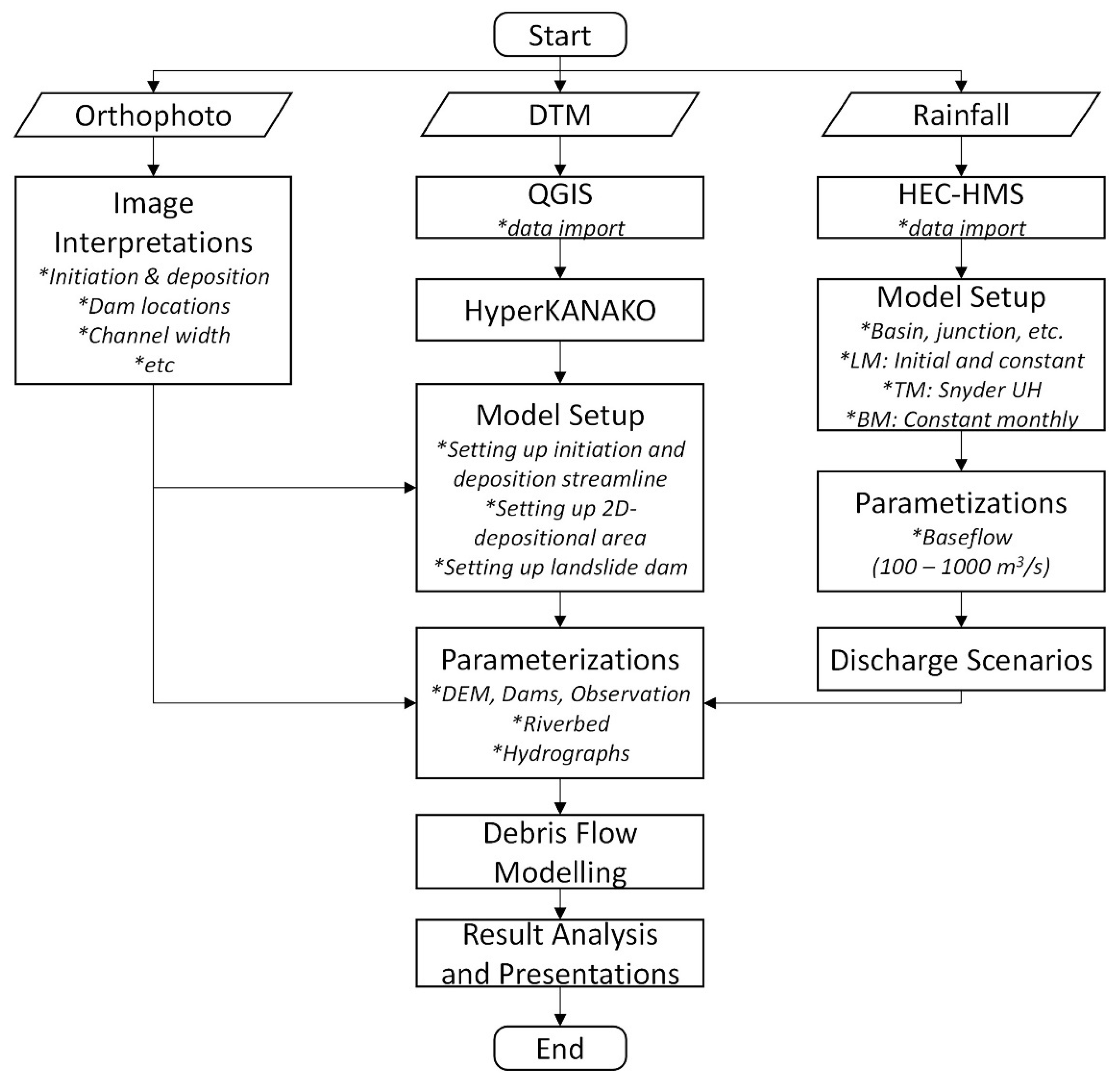
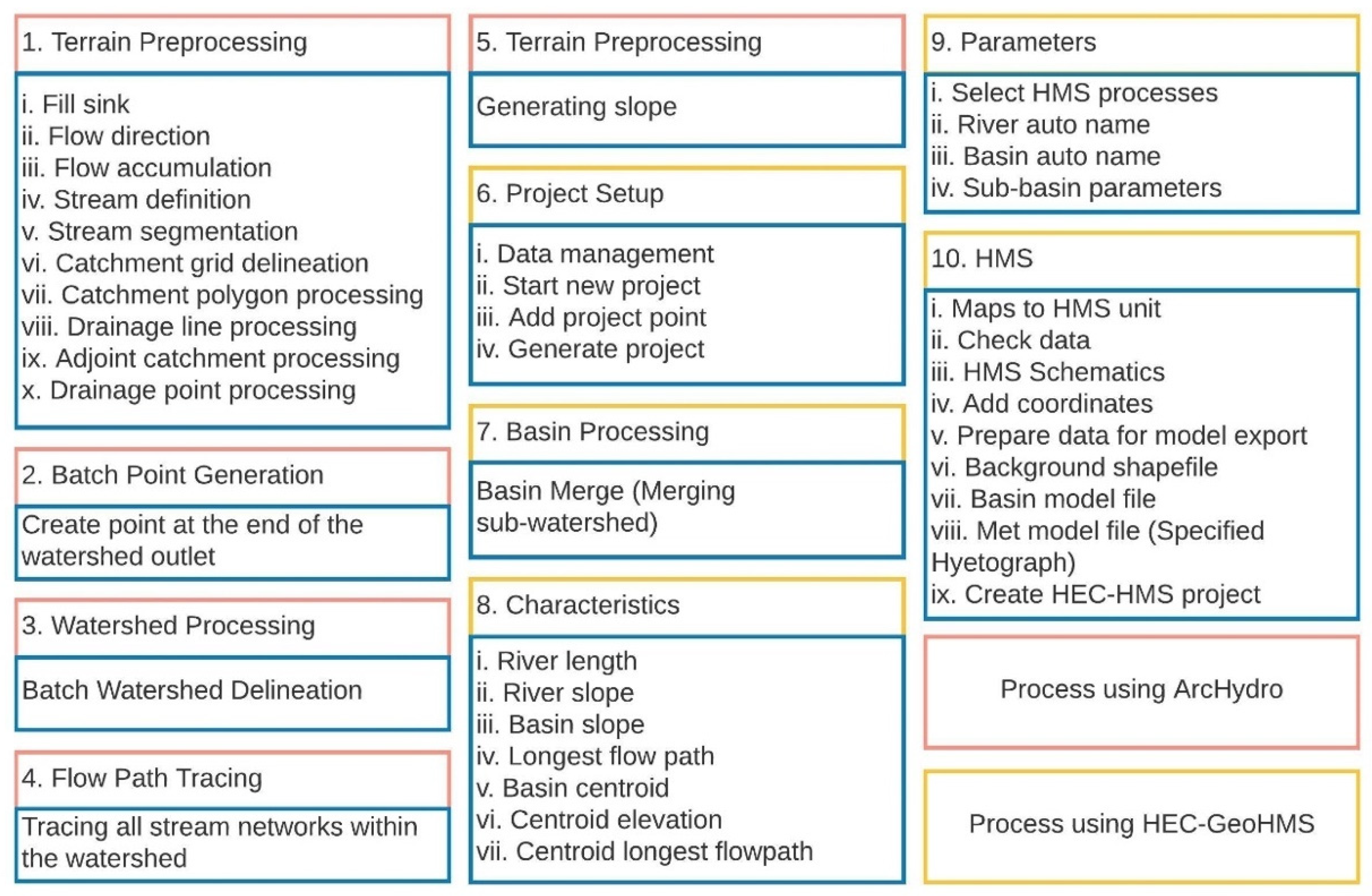
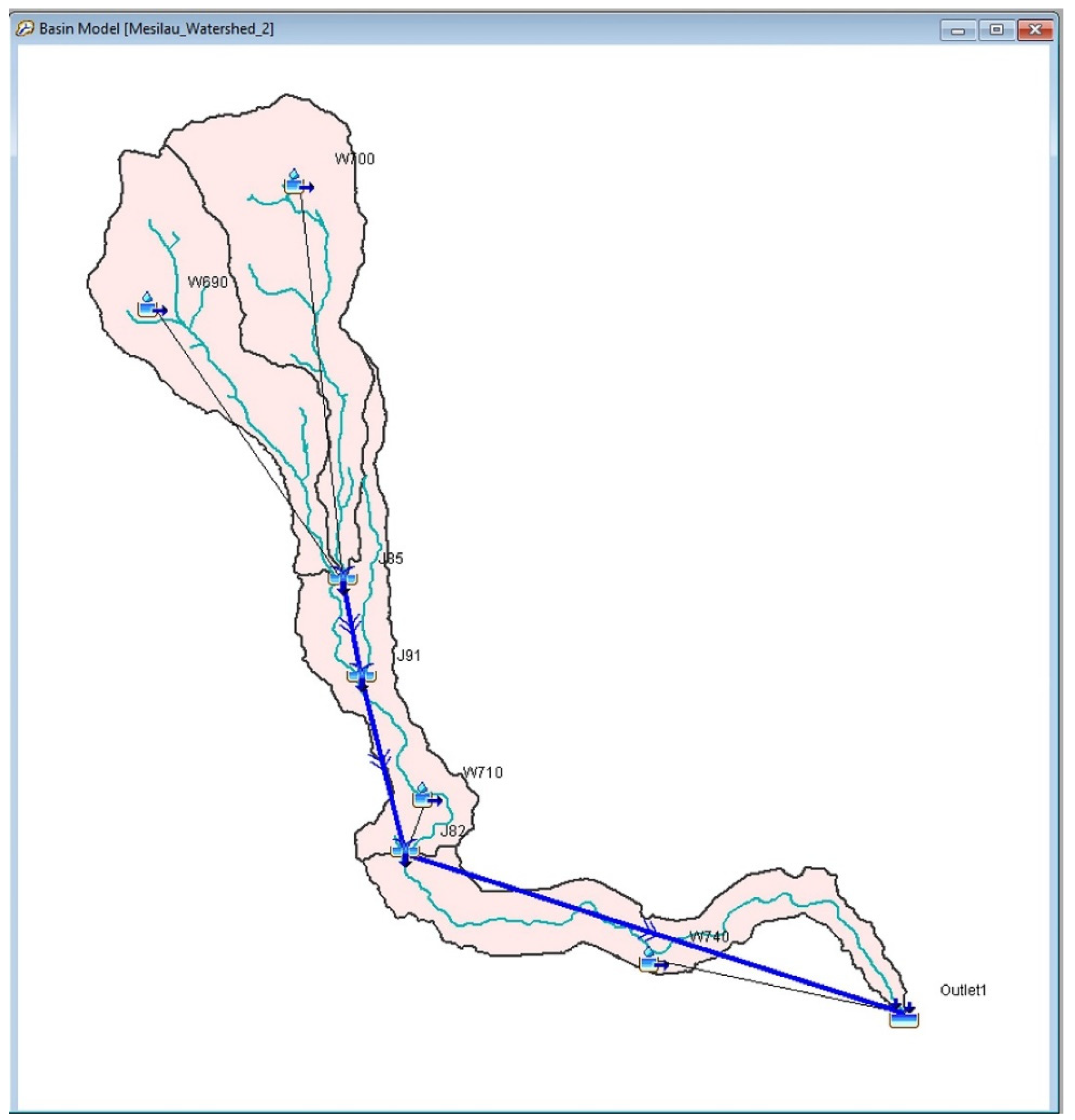
2.3. Base Model Extraction

The extraction of the base model prepared the watershed model for processing the rainfall runoff and modelling the debris flow. The base model was mainly extracted using the ArcGIS software version 10.8 with extensions of ArcHydro and HEC-GeoHMS. These extensions enabled the efficient creation of the base model in sequence following the step-wise procedures of other studies [59,60]. Figure 7 summarises the steps used to generate the base model in this study, starting with the extraction of the base model for the rainfall runoff processes. Steps 1 to 5 were conducted using the ArcHydro extension (the pink-blue rectangle), and Steps 6 to 10 were processed with the HEC-GeoHMS extension (the yellow-blue rectangle). Figure 8 shows the extracted base model; it was then exported as *.hms, and later imported into the Hydrologic Modelling System (HEC-HMS) software for processing the rainfall runoffs.

To model the debris flow, the outline shapefile of the overall watershed area (*.shp) was used to clip the raw IfSAR DTM (*.tiff) in order to obtain the boundary of the watershed area. Figure 9 shows the clipped IfSAR DTM (*.tiff) following the shapefile boundary of the watershed area (yellow). Yellow dots along the channelised river represent the distance of the past debris flow runout for every 100 m. The total debris flow runout was 18,600 m (18.6 km), with 187 dots from the initiation to the deposition area. Then, the watershed area (*.tiff) was imported into the open-source QGIS software to model the debris flow.

2.4. Rainfall Runoff Processes

Rainfall runoffs were processed with HEC-HMS software to obtain the hydrograph that triggered the debris flow event; two parameters were required by the software, i.e., the prepared base model by ArcHydro and HEC-GeoHMS extensions in ArcGIS and the hourly rainfall dataset. Figure 10 shows the workspace of the HEC-HMS software highlighting the imported base model (*.hms). Overall, the imported base model defined the basin properties, i.e., basin, sub-basin, junction, outlet, etc.

In the HEC-HMS basin model, the loss method, transform method, and baseflow method were set as the “initial and constant”, “Snyder Unit Hydrograph”, and “constant monthly”, respectively. The 2015 Ranau earthquake altered the hydrological processes within the watershed area. Water infiltrating the soil and fracturing the bedrock drained rapidly, causing large rapid flow [61]. Therefore, the initial and continuous losses were set from 1 to 5 mm based on the impervious properties of geological and land use of the watershed area.

Meanwhile, the baseflow is derived from bedrock water storage near-surface valley soils and riparian zones. Unlike the observable surface flow, the baseflow was estimated using various methods, such as tracers and baseflow separation with streamflow hydrograph. Due to the insufficient streamflow data for validation, the baseflow value was determined on a trial-and-error basis. A baseflow value of 950 m³/s for Kenyir Lake [62], the largest reservoir in Peninsular Malaysia, was used as a reference. Overall, the value for the baseflow in the Mesilau watershed was calibrated with at least ten trial-and-errors, ranging from 100 to 1000 m³/s. The Snyder Unit Hydrograph basin lag was calculated using Equation (1) below [62]:

$$t_p=C{C}_t{\left(L{L}_c\right)}^{0.3}$$

(1)

where $C_t$ is the basin coefficient (0.8), $L$ is the length of the mainstream from the farthest outlet to the divide (4.65 km), $L_c$ is the length along the mainstream from the outlet to the nearest point in the watershed centroid (2.33 km), and $C$ is the conversion constant (0.75).

The time-series data were set by importing the hourly rainfall dataset retrieved from MMD. The precipitations were assumed constant in all areas in the watershed regardless of the distance from the rainfall station.

Lastly, the control specification was set by adjusting the start/end of the date and time, and the time interval output. Following the HyperKANAKO model format, the time interval output in HEC-HMS software was set for every 60 s (1 min). The control specification allowed the software to simulate the duration of the hydrograph. Later, the ten hydrographs generated from the simulation were imported into the HyperKANAKO model to obtain the best-fit debris flow runout.

2.5. Debris Flow Modelling

The HyperKANAKO model is a debris flow simulation system that uses the debris-flow simulator KANAKO 2D developed by [46], with the flexibility of preparing datasets, user-friendly models, and an enhanced interface. Therefore, this study used this HyperKANAKO model to examine the debris flow processes and runout.

Equations for modelling included the momentum in the x-axis (Equation (2)) and y-axis (Equation (3)), the continuation of debris-flow volumes (Equation (4)), the continuation of debris flow particles (Equation (5)), and changes in the bed surface elevation (Equation (6)) [46,63]. Additionally, this model incorporated the mutual influences of the one-dimensional (1D) simulation area (i.e., gullies), and two-dimensional (2D) simulation area (i.e., alluvial fan) [64].

Equation (2) provides the momentum in the direction of the x-axis:

$$\frac{\partial u}{\partial t}+u\frac{\partial u}{\partial x}+v\frac{\partial u}{\partial y}=g\sin {\theta }_{wx}-\frac{{\tau }_x}{\rho h}$$

(2)

where $u$ is the flow velocity in the direction of the x-axis, ${\theta }_{wx}$ is the flow-surface gradient in the x-axis, ${\tau }_x$ is the riverbed shearing stresses in the x-axis, $g$ is the gravity acceleration, $\rho$ is the mass density of fluid phase, and $h$ is the flow depth.

Equation (3) describes the momentum in the direction of the y-axis:

$$\frac{\partial v}{\partial t}+u\frac{\partial v}{\partial x}+v\frac{\partial v}{\partial y}=g\sin {\theta }_{wx}-\frac{{\tau }_y}{\rho h}$$

(3)

where $v$ is the flow velocity in the direction of the y-axis, ${\theta }_{wx}$ is the flow-surface gradients in the y-axis, and ${\tau }_y$ is the riverbed shearing stresses in the y-axis.

The continuation of debris-flow volume was computed using Equation (4) as follows:

$$\frac{\partial h}{\partial t}+\frac{\partial uh}{\partial x}+\frac{\partial vh}{\partial y}=S_T$$

(4)

where $S_T$ is the sediment erosion or the deposition velocity. The continuation of debris flow particles was calculated by Equation (5):

$$\frac{\partial Ch}{\partial t}+u\frac{\partial Cuh}{\partial x}+v\frac{\partial Cvh}{\partial y}=S_T{C}_{*}$$

(5)

where $C$ is the sediment concentration by volume in the debris flow and $C_{*}$ is the sediment concentration by volume in the moveable bed layer.

The determination of changes in the bed elevation was based on Equation (6) as follows:

$$\frac{\partial z}{\partial t}+S_T=0$$

(6)

where z is the bed elevation.

Meanwhile, the model setup, began with the streamline within the initiation and deposition area. The initiation line of this study was located in the landslide dam, whereas the deposition line was within the Liwagu Dam of the Ranau town. A green line and a yellow rectangle were displayed on the workspace, representing the expected runout and the deposition area, respectively. Subsequently, the deposition area was adjusted by changing the mesh sizes of the x- and y-axes until the debris flow was projected to be deposited in the Liwagu Dam. Figure 11 shows the model setup within the study area. The type of dam and its heights were set within the initiation and deposition area, respectively. The heights of the post-landslide dam and the Liwagu Dam were measured using the laser-range finder during a field investigation on 31 August 2019. The landslide dam within the initiation area was set to the height of 30.0 m (Figure 12a), while the closed dam within the downstream area was adjusted to a height of 5.0 m (Figure 12b).

Additionally, the modelling parameters were calibrated through the open-source LibreOffice 5 software with three primary tabs, i.e., the “DEM, Dams, and Observation”, “riverbed”, and “hydrograph”.

Table 3. The calibrated parameters in the “DEM, Dams, and Observation” tab.

Parameters/Variables	Value	Unit
Simulation time	40	min
Time step	1	s
Diameter of material	1	m
Mass density of bed material	2650	kg/m3
Mass density of fluid	1200	kg/m3
Concentration of moveable bed	0.2	-
Internal friction angle	35	degree
Acceleration of gravity	9.8	m/s2
Coefficient of erosion rate	0.0007	-
Coefficient of deposition rate	0.05	-
Manning’s roughness coefficient	0.03	s/m1/3
Number of calculation points	250	-
Interval of 1D calculation points	5	m
Number of 2D calculation points	480 × 160	-
Interval of 2D calculation points	5 × 5	m × m

shows the calibrated parameters for the “DEM, Dams, and Observation”; these parameters were calibrated by reviewing the available historical records of the study area with modifications based on global events, such as Japan [63,65] and Indonesia [66]. Additionally, several parameters, such as mass density of bed materials, mass density of fluids, coefficient of erosion and deposition rate, and acceleration of gravity of the study area were set as the default. For the “riverbed”, the average channel width was adjusted to 5.0 m upon crosschecking the orthophoto and DEM before and after the debris flow event by changing the value in the riverbed. Table cross-sections were prepared for every 100 m (the yellow dots) to evaluate the channel width. Finally, the hydrograph generated from the HEC-HMS was imported into the relevant tab by manually inserting these values for every timestamp.

Additionally, a sensitivity analysis was conducted to attain the best-fit debris flow runout for the past event with ten simulated scenarios by importing ten hydrographs acquired through the HEC-HMS. Indicators for evaluating the runouts included the flow depth, depositional thickness, and runout distance. The flow depth was evaluated along the Mesilau Nature Resort bridge (upstream area), whereas the depositional thickness and runout distance were observed within the Liwagu Dam (downstream area). The best-fit debris flow runout was presented in a spatial map.

3. Results

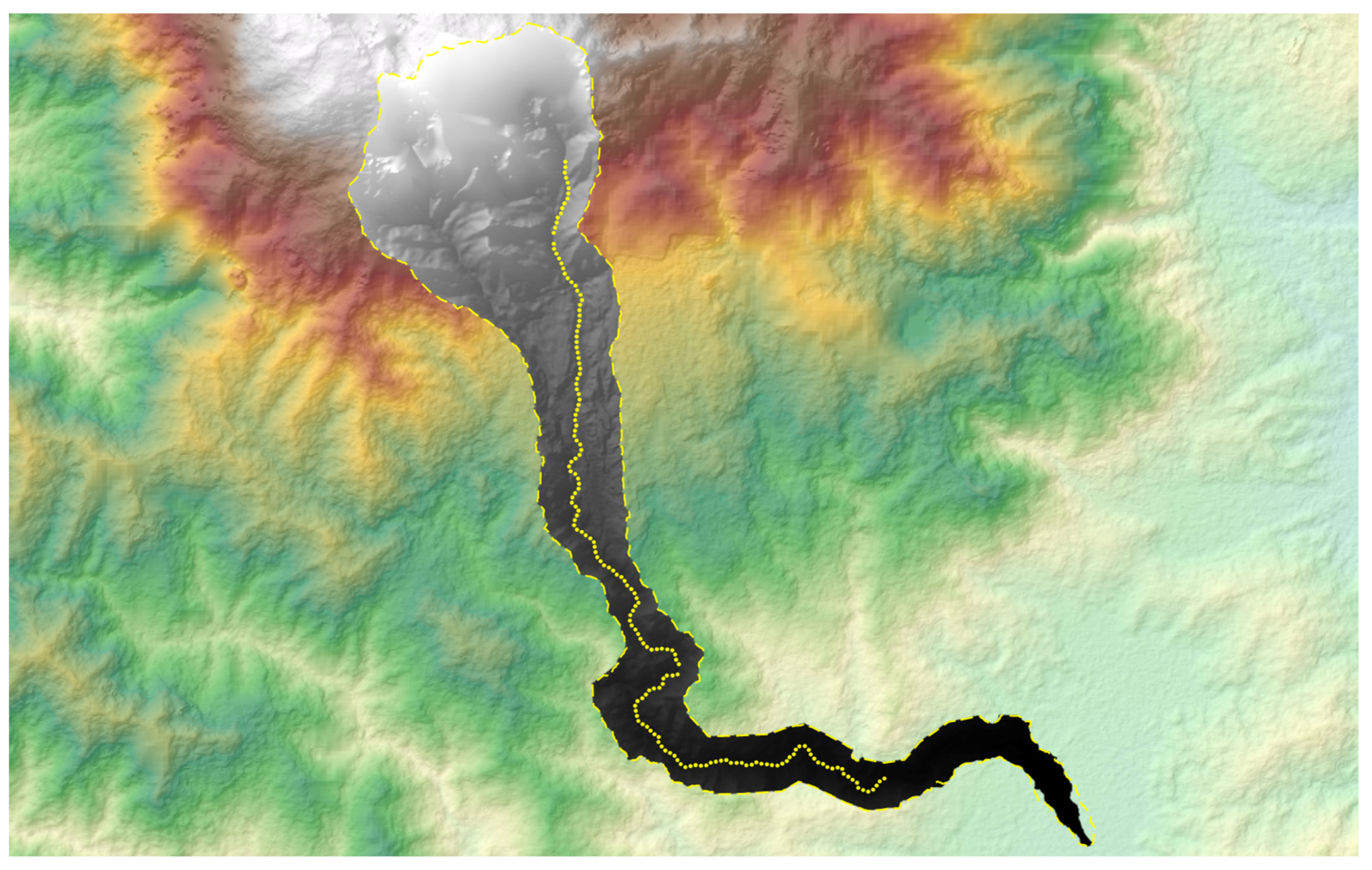
3.1. Best-Fit Debris Flow Runout

Table 4. The 11 summarized simulation scenarios by varying the baseflow and hydrographs.

Scenario	Baseflow (m3/s)	Hydrograph (m3/s)	Simulation Runout Distance
Scenario 1	100	113.8	Short
Scenario 2	200	213.8	Short
Scenario 3	300	313.8	Short
Scenario 4	400	413.8	Short
Scenario 5	500	513.8	Almost reach
* Scenario BF	550	563.8	Best-fit
Scenario 6	600	613.8	Over-estimate
Scenario 7	700	713.8	Over-estimate
Scenario 8	800	813.8	Over-estimate
Scenario 9	900	913.8	Over-estimate
Scenario 10	1000	1013.8	Over-estimate

* represents the best-fit simulation result.

summarizes the simulation results for the ten different scenarios. Overall, the runout distance increased along with the hydrographs. For example, Scenarios 1 to 4 produced short runouts, whereas Scenarios 6 to 10 yielded overestimated runouts. The best-fit runout happened between Scenarios 5 and 6, and both scenarios were nearly similar to the past event. Therefore, the recalibration was conducted for the parameters between Scenarios 5 and 6 to produce the best-fit debris flow runout labelled as “Scenario BF”. The result shows that the best-fit debris flow runout was obtained as a hydrograph of 563.8 m³/s and a baseflow of 550 m³/s.

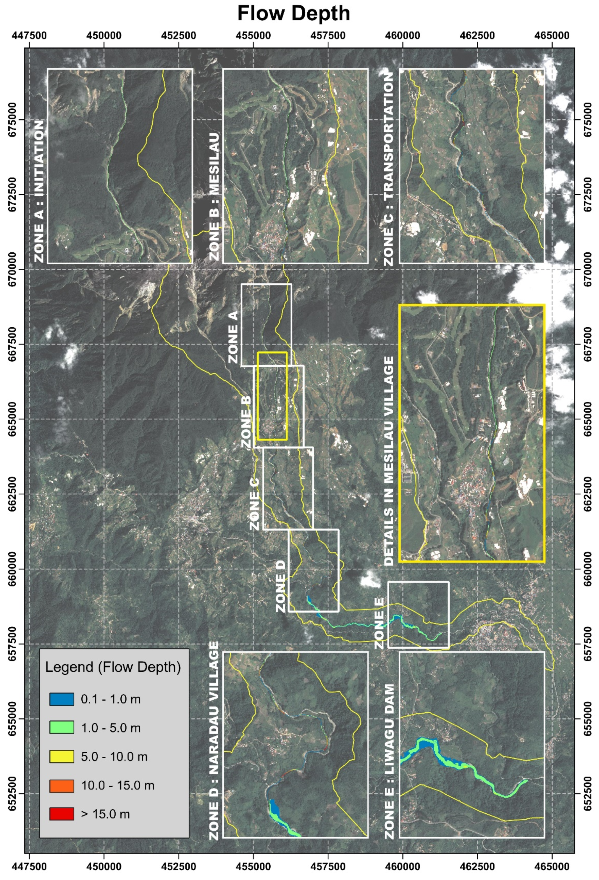
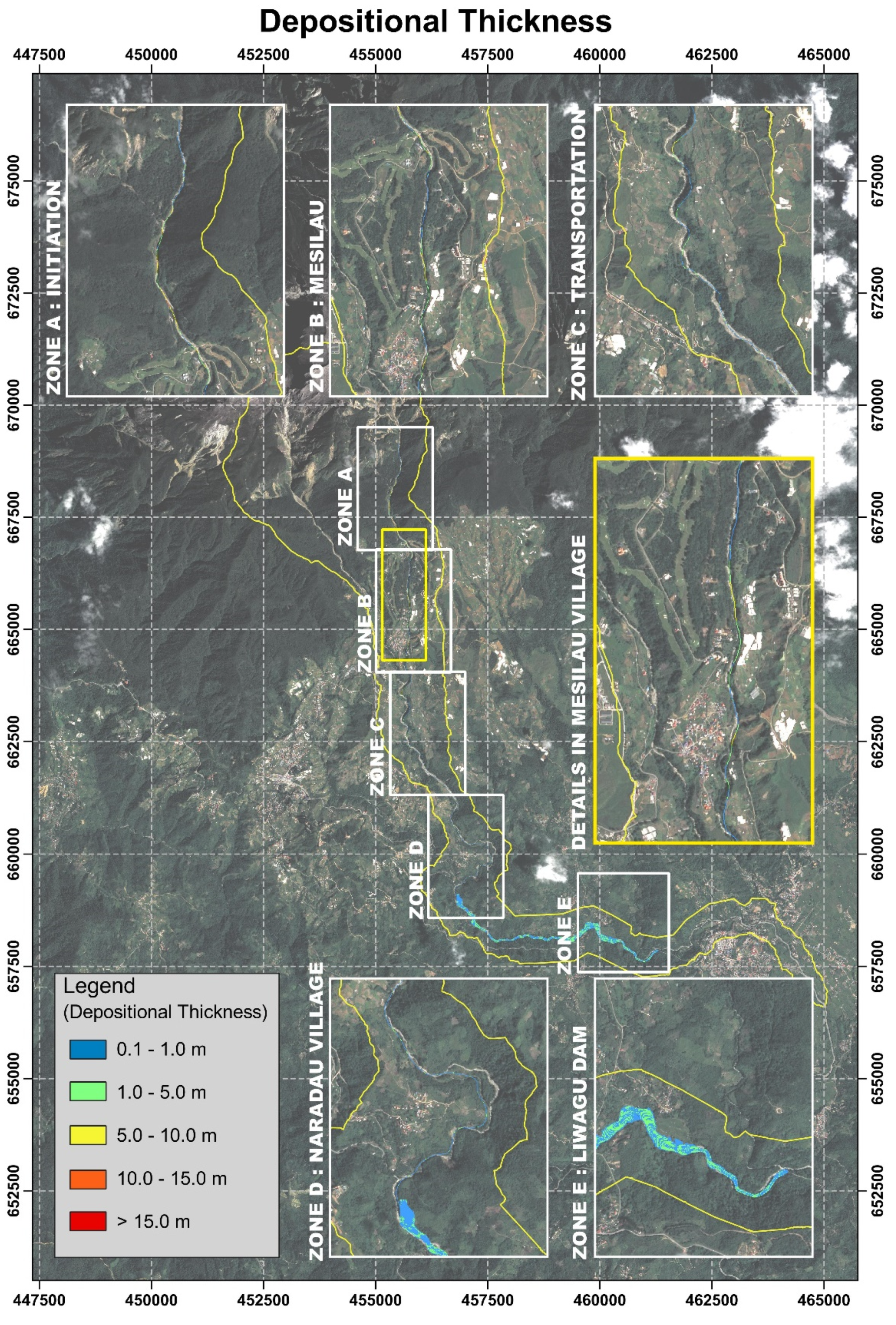
3.2. Flow Depth and Depositional Thickness of Best-Fit Runout

Figure 13 and Figure 14 show the flow depth and depositional thickness of the best-fit debris flow runout, respectively. As highlighted, a multicoloured line was visualised along the channel, and each colour represented different ranges of flow depths and depositional thickness. These maps also show five different zones, highlighting significant areas, such as Zone A (initiation area), Zone B (Mesilau village), Zone C (transportation area), Zone D (Naradau village), and Zone E (Liwagu Dam).

Table 5. The flow depth of every zone.

Zones	Colour Range	Flow Depth (m)
Zone A (Initiation area)	green to orange	1.0–15.0
Zone B (Mesilau village)	green to yellow	1.0–10.0
Zone C (Transportation area)	blue to yellow	0.1–10.0
Zone D (Naradau village)	blue to green	0.1–5.0
Zone E (Liwagu Dam)	blue to green	0.1–5.0

and

Table 6. The depositional thicknesses for every zone.

Zones	Colour Range	Depositional Thickness (m)
Zone A (Initiation area)	green to orange	1.0–15.0
Zone B (Mesilau village)	blue to yellow	0.1–10.0
Zone C (Transportation area)	blue to green	0.1–5.0
Zone D (Naradau village)	blue to green	0.1–5.0
Zone E (Liwagu dam)	blue to green	0.1–5.0

summarise the flow depth and depositional thickness, respectively, for each zone. For a detailed evaluation, the flow depth was analysed in Zone B during the transportation process, whereas the depositional thickness was focused on Zone E after the simulation had ended. These two areas were selected based on the field data inputs and evidence collected by interviewing the eyewitnesses of the debris flow event and obtaining input from local communities.

The flow depth within Zone B was most frequently observed and marked by the green line with flow depths of 1.0 to 5.0 m; the least visualised zone was represented by the yellow line with a flow depth ranging from 5.1 to 10.0 m (Figure 13). Additionally, the flow depth did not overflow from the channel bank, indicating that the simulation result was congruent with the past event. Interviews with the local community further supported flow depth by justifying the highest depth within the channel banks during the event, especially along the village area (Figure 13).

The depositional thickness of Zone E, mostly highlighted with the blue to green line, ranged from 0.1 to 5.0 m (Figure 14). The widespread of blue line within the Liwagu Dam was indicative of the overflowing debris from the channel bank (Figure 14).

3.3. Estimated Velocity and Lead Time

The best-fit runout was also used to estimate the debris-flow velocity and the lead time to arrive at the nearest villages, i.e., Mesilau village, Naradau village, and Ranau town. The estimated channel distance from the landslide dam (the initiation area) to the nearest villages were 3.9 km, 11.1 km, and 18.6 km, respectively. The estimated average debris flow velocity derived from the simulation result was 12.5 m/s. The lead time to arrive at each village was 4.5 min, 14 min, and 24 min, respectively. The analysis showed that the local community of Mesilau village would have the shortest time of 4.5 min to evacuate as compared with the Naradau village and Ranau town. This finding would be crucial for designing an early warning system (EWS) to disseminate risk information and the evacuation route.

4. Discussion

This study investigated the debris flow runout triggered by the prolonged rainfall after the 2015 Ranau earthquake in the Mesilau watershed, Kundasang, Sabah. To date, this is the first study conducted within East Malaysia to simulate the past debris flow in the vicinity of Mount Kinabalu. This study provides better insights into debris flow characteristics, including the estimated velocity, lead time, flow depth, and depositional thickness, which would allow the development of debris flow prevention and mitigation measures. Thus far, no EWS has been installed in the area, which increases the likelihood of future debris flows with mild seismic activity and rainfall.

Overall, the debris flow in this area was different from other reported events, such as Genting Sempah, Gunung Pulai, and Pos Dipang [9,14,19] as the source materials (i.e., sediment and debris) of this area were induced by the earthquake and later remobilised as a debris flow following a seven-day prolonged rainfall (66.3 mm) and least amount of rainfall intensity (14.2 mm/h). Consequently, a long debris flow runout of 18.6 km was recorded flowing from the foot slope of Mount Kinabalu until the Liwagu Dam of Ranau town. This debris flow permanently changed the river morphology, disrupting critical infrastructures (e.g., bridges, roads, and dams), degrading the water quality, and affecting socioeconomic activities.

The HyperKANAKO model used in this study was sensitive towards the hydrographs, i.e., the hydrographs increased along with flow depths, depositional thickness, and runout distance. The best-fit debris flow runout, recalibrated between Scenarios 5 and 6, showed that the past debris flow had a discharge of 563.8 m³/s, mostly derived from the baseflow of 550 m³/s, indicating that the least amount of rainfall was enough to trigger the debris flow after the earthquake in the Mesilau watershed. The baseflow value of 550 m³/s for the Mesilau watershed was reasonable as it was less than the baseflow for water bodies [62]. Additionally, the estimated debris flow velocity and the lead time to arrive at the nearest Mesilau village were 12.5 m/s and 4.5 min, respectively. Due to its high debris-flow velocity, this study recommends a community evacuation of 4.5 min before the debris flow arrives in the village. Since the evaluated lead time of 4.5 min is too short for the community to complete the evacuation, there is a need to develop an impact-based multi-hazard EWS for disseminating the warning message as early as possible. Additionally, an early detection system on natural or landslide dams in the highland area is suggested. Once the emergence and growth of landslide dams are detected, a warning should be issued for the community to evacuate from high-risk areas before the commencement of debris flow. The EWS is proposed for the watershed area following the Malaysia’s initiative to achieve the global targets of the Sendai Framework for Disaster Risk Reduction 2015–2030.

The simulation results of this study show that the flow depth within Zone B (Mesilau village) was below 10.0 m, and this result was congruent with past evidence. Then, the flow depth gradually decreased as it travelled to Zones C, D, and E. Meanwhile, the depositional thickness ranged from 0.1 to 5.0 m within Zone E (Liwagu Dam), probably due to the accumulated debris within the closed dam.

These results (i.e., reconstruction of past events, flow depth, depositional thickness, debris flow velocity, and lead time) might serve as baseline data to create greater awareness among local stakeholders and vulnerable communities towards understanding the past debris flow event for preventing future risks. This study is timely and significant as the earthquake return period is approximately 25 years in the Ranau district, which might trigger future debris flows in the area [57]. Thus, further studies are needed to include more parameters for modelling debris flow and to design suitable structural and nonstructural mitigation measures in the localised area. An integrated framework is critically needed for responding to sediment-related disasters, as the area is highly vulnerable to future debris flow given the active tectonic activities, hanging rocks in the mountains due to geodynamic activity, and high exposure to typhoons and their hydrometeorological impact.

5. Conclusions

This study modelled the past debris flow in the Mesilau watershed by applying several interrelated processing platforms, including ArcGIS (ArcHydro and HEC-GeoHMS), HEC-HMS, QGIS, and HyperKANAKO. On the basis of the observation data and the best-fit simulation result, it can be concluded that:

(1)

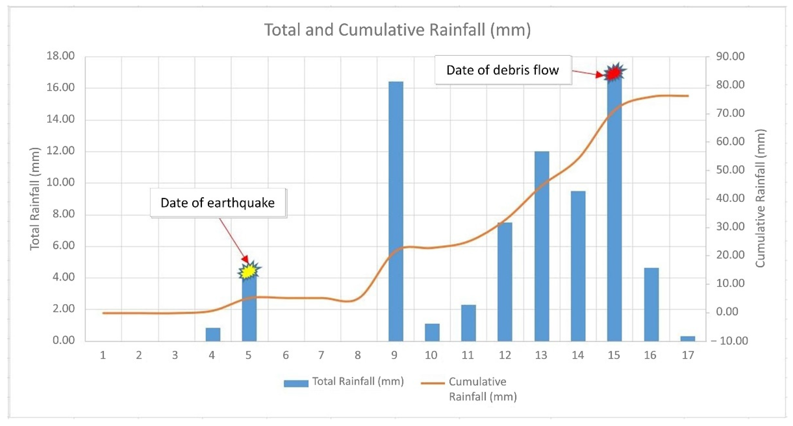
The debris flow happened on 15 June 2015, i.e., ten days after the 2015 Ranau earthquake (Mw 6.0) with a seven-day cumulative rainfall of 66.3 mm. The maximum rainfall intensity was 14.2 mm/h; it breached the landslide dam and initiated the debris flow. The early identification showed that the least amount of rainfall was sufficient to trigger the debris flow after the earthquake in the Mesilau watershed.

(2)

According to the best-fit simulation, the debris flow velocity was estimated to be 12.5 m/s and the lead time to arrive at the nearest Mesilau village was 4.5 min, representing the required evacuation time by the community to minimise the debris flow impacts and prevent human losses.

(3)

Additionally, the baseflow during the past event was 550 m³/s, yielding a discharge of 563.8 m³/s. According to the reference value of the Kenyir lake [62], the baseflow for the Mesilau watershed should not exceed the baseflow of water bodies, i.e., 950 m³/s.

(4)

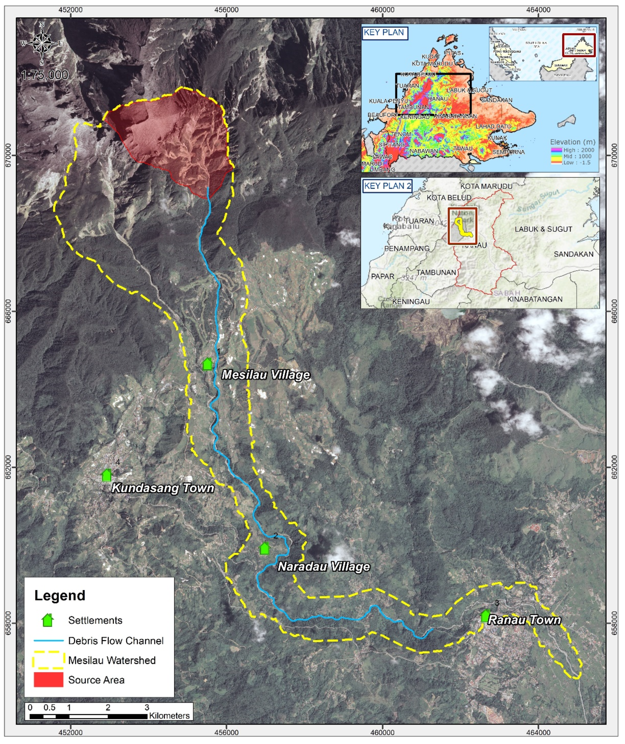
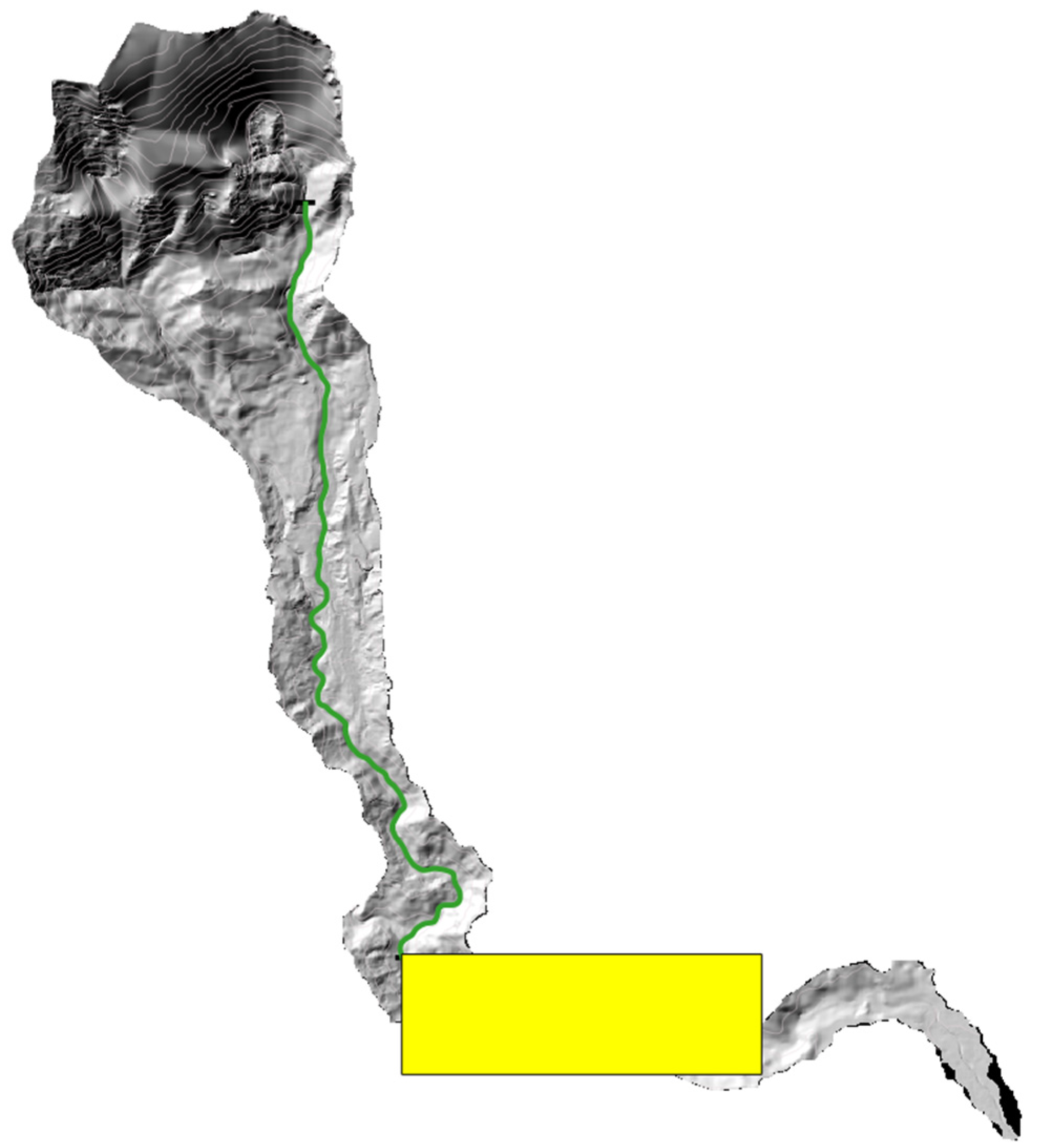
The approximate runout distance flowing from the landslide dam to the Liwagu Dam of the Ranau town was 18.6 km, due to a large amount of sediment supply (accumulated debris) generated during the 2015 Ranau earthquake.

(5)

As the debris began flowing, the flow depth gradually decreased from 15.0 m at the initiation area to 5.0 m at the deposition area. In Zone B (the Mesilau village), the flow depth ranged from 1.0 to 10.0 m with no overflowing debris identified. In Zone E (the Liwagu Dam), the depositional thickness was less than 5.0 m; the closed dam blocked the accumulated debris along the channel.

There was some degree of uncertainty while simulating the event since assumptions and empirical laws were used based on the inputs that the HyperKANAKO model requires. Although debris flow runout models have been used with regularity in the past to re-establish past events via the calibration of input parameters, there are still some limitations in the physical description. Therefore, future research is needed for both physical and modelling studies, especially the complex processes and mechanism of debris flow in this earthquake-prone area in order to quantify and to reduce uncertainty.

Predictive assessments may facilitate improved management of future debris flow, and therefore reduce the hazard. This study supports the commitment of the Malaysia Government to achieve the global targets of Sendai Framework for Disaster Risk Reduction 2015–2030 particularly the Global Target G-5 on the accessible, understandable, usable, and relevant disaster risk information, which can later be used to design and develop the multi-hazard EWS. Nonstructural mitigation measures such as early warning systems might allow the local government to estimate the percentage of the population exposed to or at risk from disasters and protect them through preventive evacuation following early warning (Global Targets G1, G3, G4, and G6), and to develop local disaster risk reduction and resilience strategies (Global Target E2) [67].