A Theoretical Study of the Hydrodynamic Performance of an Asymmetric Fixed-Detached OWC Device

Abstract

The chamber configuration of an asymmetric, fixed-detached Oscillating Water Column (OWC) device was investigated theoretically to analyze its effects on hydrodynamic performance. Two-dimensional linear wave theory was used, and the solutions for the associated radiation and scattering boundary value problems (BVPs) were derived through the matched eigenfunction expansion method (EEM) and the boundary element method (BEM). The results for the hydrodynamic efficiency and other important hydrodynamic properties were computed and analyzed for various cases. Parameters, such as the length of the chamber and the thickness and submergence of the rear and front walls, were varied. The effects on device performance of adding a step under the OWC chamber and reflecting wall in the downstream region were also investigated. A good agreement between the analytical and numerical results was found. Thinner walls and low submergence of the chamber were seen to increase the efficiency bandwidth. The inclusion of a step slightly reduced the frequency at which resonance occurs, and when a downstream reflecting wall is included, the hydrodynamic efficiency is noticeably reduced at low frequencies due to the near trapped waves in the gap between the OWC device and the rigid vertical wall.

1. Introduction

Ocean wave energy is a renewable and pollution-free resource with the potential to mitigate the effects of global warming and contribute to meet the world’s growing demand for electricity. This globally available energy source is estimated at about 2.1 TW [1], or 18,400 TWh per year, approximately 80% of the 2018 world’s demand for electricity [2]. By use of wave energy converters (WECs), this energy source can be collected and transformed into electricity. In recent decades a broad range of WEC technologies has been proposed, with the Oscillating Water Column (OWC) device emerging as one of the most successful systems for wave energy harvesting.

The OWC differs from other technologies in its simple operating principle and adaptability for a range of locations (on the coastline, in the nearshore region or offshore). Thus, OWC systems have been researched most often, with full-scale prototypes being developed a number of times [3]. The system essentially consists of two components: a partially submerged hollow structure into which water enters through a bottom opening, and a Power Take-Off (PTO) mechanism, which converts the wave energy into electrical energy. Typically, the PTO system is a Wells turbine, which is the only moving element of the mechanism and which is above the level of the seawater to avoid direct exposure. The hollow chamber has a water column and an air column. The working principle is analogous to a piston in a cylinder; the trapped water inside is forced to oscillate up and down by the wave action. This alternately compresses and rarefies the air, trapped above the water column, and drives the airflow back and forth across the turbine in a duct that is coupled to a generator [4].

In an OWC system, wave energy is absorbed by a hydrodynamic mechanism involving relatively complex diffraction and radiation wave processes [3]. In recent years, many researchers have studied the hydrodynamic performance of the OWC device using theoretical analysis, experimental tests, and numerical simulations. Pioneering studies of wave energy absorbers based on rigid body models were performed by [5,6,7,8]. Earlier, studies of the parameters affecting the hydrodynamic efficiency of land fixed OWC devices were conducted by [9,10,11,12,13,14].

Pile-supported OWC structures, with hydrodynamic behavior similar to fixed-detached devices, have been widely studied as a means of extracting wave energy for electricity generation and reducing wave transmission, mainly through the mechanisms of wave reflection [15,16,17,18,19,20,21]. The performances of pile-supported and land-fixed OWC devices were analyzed in experiments by [15]. A pile-supported OWC-type breakwater was experimentally investigated by [16]. They found that greater pneumatic damping increased energy extraction, but that with less pneumatic damping energy dissipation was more efficient in vortex-induced energy loss. He and Huang [17] investigated the hydrodynamic performance of a pile-supported OWC structure in front of a vertical wall, demonstrating that this system can serve as a wave absorber to reduce the wave reflection from vertical walls. He et al. [18] employed the matched EEM to investigate the hydrodynamics of a pile-supported OWC breakwater. Their results showed that by adjusting PTO damping for maximum power, adequate power extraction and wave transmission is possible, whereas optimizing PTO damping for minimal wave transmission significantly lowers power extraction. The combined effect of the chamber geometry and wave conditions on the performance of fixed-detached and asymmetric OWC devices was investigated by [22]. Qu et al. [23] performed experimental tests to study an integrated OWC-pile-supported permeable breakwater and found that, compared with a non-permeable scheme, wave power generation and environmental protection performance were better.

Extensive investigations have been conducted on offshore fixed OWC system performance [24,25,26,27,28]. Ref. [24] performed both experimental test and numerical simulations of a 3D offshore stationary OWC device subjected to regular waves. They showed that the total power extraction efficiency of an offshore OWC is considerably overestimated by 2D and wave flume modelling, especially for wave frequencies greater than the chamber resonant frequency. Elhanafi et al. [25] investigated the effects of the underwater front and rear lips on the hydrodynamic performance of an offshore stationary OWC using a computational fluid dynamics (CFD) model. They concluded that by selecting an appropriate submergence ratio of the asymmetric lips and lip thickness, the total hydrodynamic efficiency is considerably increased for a broad bandwidth frequency. Experimental tests were carried out by [28] on a fixed offshore OWC model to study the effect of the wave spectrum shape on its efficiency. An analytical model to analyze the effects of a skirt on an OWC device integrated into an offshore wind turbine monopile was carried out by [29]. Through both experimental tests and numerical simulations, Deng et al. [30] studied the hydrodynamic performance of an offshore-stationary OWC device with an immersed horizontal bottom plate. By means of the EEM, Deng et al. [31] made a theoretical study of an asymmetric, offshore-stationary OWC device with an outstretched bottom plate. They found that the bottom plate provides an additional resonance mechanism that can be adjusted to offer a wider bandwidth with high performance.

There is still a lot to be investigated regarding the improvement of the hydrodynamic efficiency of fixed-detached OWC devices by modifying the geometric parameters of the chamber. To the best of the authors’ knowledge, a theoretical study into the interaction of water waves with a fixed-detached OWC device with asymmetric thick rear and front walls, with a step and a reflecting wall, has not been reported. Apart from absorption of wave energy, fixed-detached OWC devices can be used to protect maritime structures and human activities from wave attack, as well as to enable water exchange and sediment transport [16]. They may, however, be affected by severe storms, which can cause serious structural damage, as was the case with the Mutriku Wave Energy Plant [32]. Therefore, the thickness of the back and front barriers that comprise the OWC chamber must be designed to withstand wave loads and save the structure, while the effect that this would have on the device performance must be also considered.

Compared to experimental and CFD approaches, this theoretical investigation has the advantage of quickly evaluating different parameters of a fixed-detached OWC device. The main objectives of this analysis were to examine modifications in bandwidth on the efficiency curves and the shifting of the peak resonant frequency due to different rear and front wall configurations, chamber size, and the length of the gap between the OWC chamber and the reflecting wall.

The present study is organized as follows: Section 2 defines the physical problems corresponding to the water wave radiation and scattering by a fixed-detached OWC device, based on the potential flow theory. In Section 3 the methodologies for solving the BVPs are presented. First, the matched EEM is described, where the eigenfunction expansions along with their orthogonal properties, the continuity of velocity potential, and flux are used to reduce the BVP into a linear system of algebraic equations. Then the BEM, which is a numerical technique based on an integral equation formulation and boundary discretization, is presented. In this work, the BEM with three-noded elements is used to account for the variation of the potential and flux on the boundaries. Section 4 describes the procedure for obtaining the energy relations. In Section 5 and Section 6, convergence and truncation analyses are carried out, respectively, and a comparison is made with the experimental results of [16,17]. Section 7 shows the results for various modelled cases. Finally, in Section 8, the main conclusions of this study are drawn.

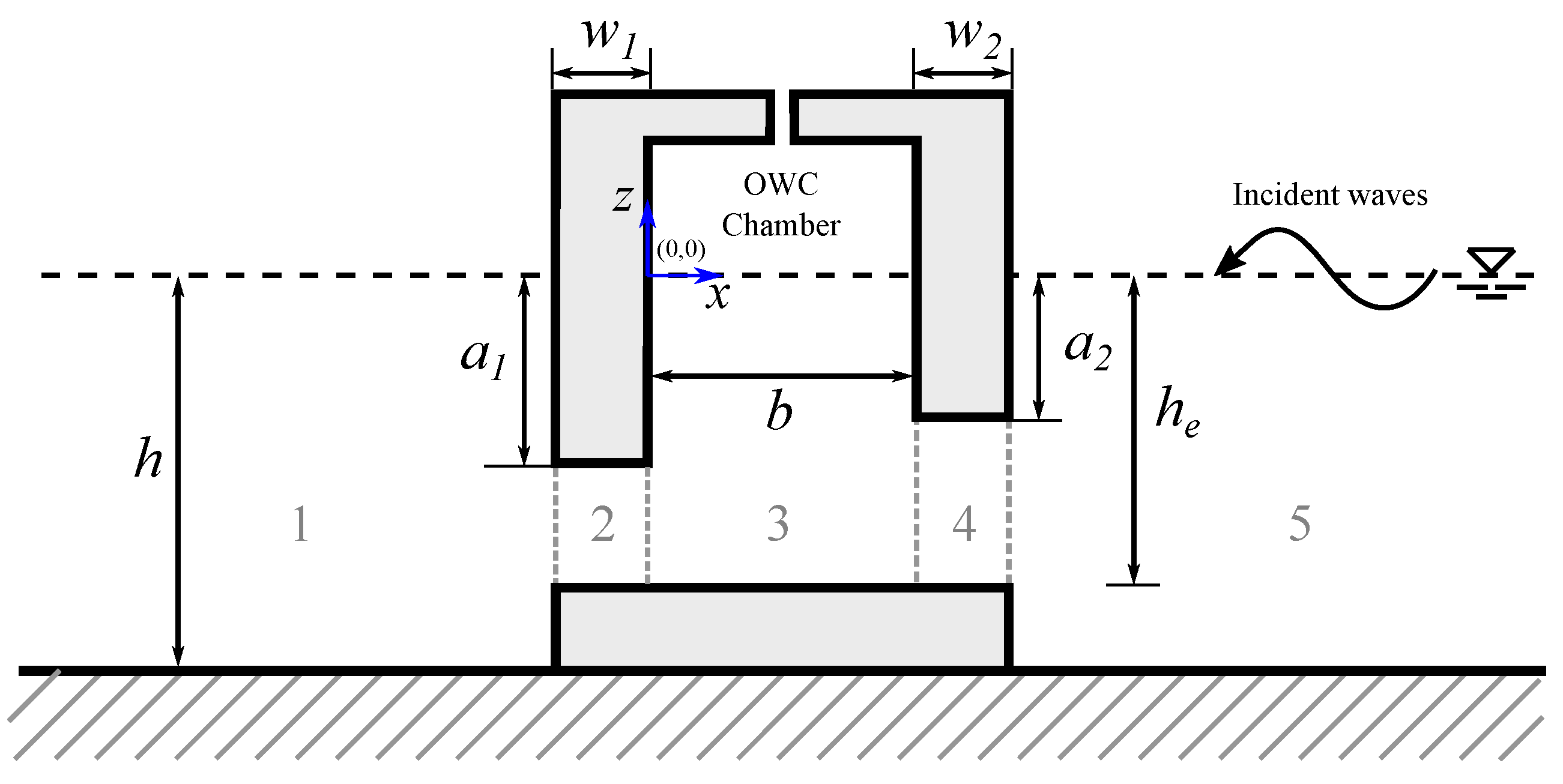
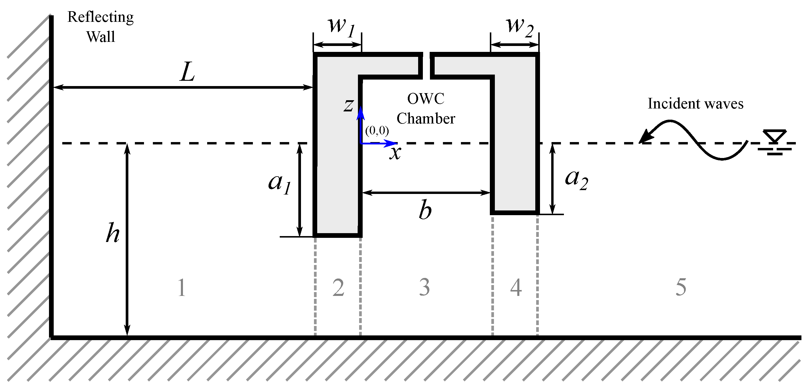
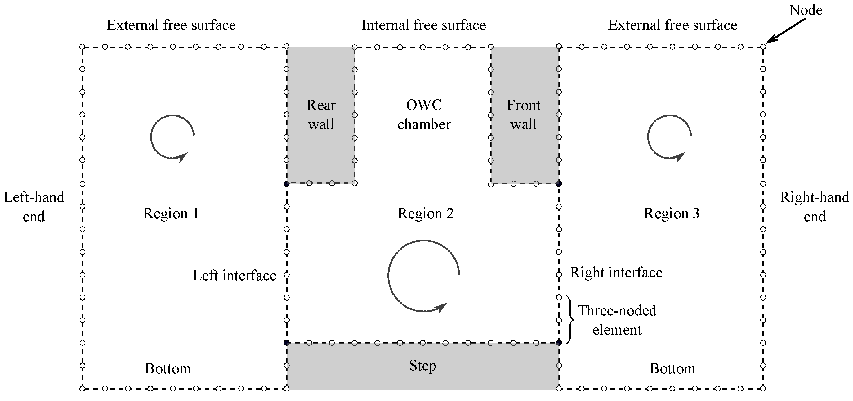
2. Boundary Value Problem

Figure 1 shows the fixed-detached OWC device, the fluid and the Cartesian coordinate system, with the vertical coordinate, z, measured positively upwards and the undisturbed free surface located at $z=0$. The waves approach the device from the positive x direction. The device is composed of two partially immersed front and rear walls, separated by distance b. The rear wall is located at $x=-w_1$, with a draft $a_1$ and a thickness $w_1$, while the front wall is located at $x=b$, with draft $a_2$ and thickness $w_2$. A step under the OWC device is considered with a height $h-h_e$. There is assumed to be a turbine connecting the trapped air inside the chamber and the atmosphere.

The BVP is divided into five regions, as shown in Figure 1, and the boundaries are denoted by

• The rear wall by $B_r=\{(x,z):(x=-w_1,-a_1\le z\le 0)\cup (-w_1<x<0,z=-a_1)\cup (x=0,-a_1\le z\le 0)\}$.
• The front wall by $B_f=\{(x,z):(x=b,-a_2\le z\le 0)\cup (b<x<f_w,z=-a_2)\cup (x=f_w,-a_2\le z\le 0)\}$ where $f_w=b+w_2$.
• The internal free surface inside the chamber by $F_i=\{(x,z):(0\le x\le b,z=0)\}$.
• The external free surface by $F_e=\{(x,z):(-\infty <x<-w_1,z=0)\cup (f_w<x<\infty ,z=0)\}$.
• The bottom by $B_d=\{(x,z):(-\infty <x<-w_1,z=-h)\cup (x=-w_1,-h\le z\le -h_e)\cup (-w_1<x<f_w,z=-h_e)\cup (x=f_w,-h\le z\le -h_e)\cup (f_w<x<\infty ,z=-h)\}$.

The fluid is inviscid and incompressible and the flow is irrotational; thus, the velocity potential theory is applied. The wave motion is represented by linearized wave theory, disregarding surface tension effects. A simple harmonic flow with angular frequency $\omega$ is assumed, where the velocity potential is defined by $\mathsf{\Phi }(x,z,t)$ with $\mathsf{\Phi }(x,z,t)=\mathrm{Re}\left\{\varphi (x,z){\mathrm{e}}^{-\mathrm{i}\omega t}\right\}$, with Re$\left\{\right\}$ denoting the real part of a complex expression. Under these assumptions, the spatial velocity potential $\varphi$ satisfies the Laplace equation

$$\left(\frac{{\partial }^2}{\partial x^2}+\frac{{\partial }^2}{\partial z^2}\right)\varphi =0.$$

(1)

The no-flow boundary conditions are applied at the bottom and the two barriers as

$$\frac{\partial \varphi }{\partial n}=0\mathrm{for}(x,z)\in B_d,B_r\mathrm{and}{B}_f,$$

(2)

The continuity of pressure and horizontal velocity on the common interfaces of the five regions are given by

$${\varphi }_1={\varphi }_2\mathrm{and}\frac{\partial {\varphi }_1}{\partial x}=\frac{\partial {\varphi }_2}{\partial x}\mathrm{on}x=-w_1\mathrm{and}-h_e\le z\le -a_1,$$

(3a)

$${\varphi }_2={\varphi }_3\mathrm{and}\frac{\partial {\varphi }_2}{\partial x}=\frac{\partial {\varphi }_3}{\partial x}\mathrm{on}x=0\mathrm{and}-h_e\le z\le -a_1,$$

(3b)

$${\varphi }_3={\varphi }_4\mathrm{and}\frac{\partial {\varphi }_3}{\partial x}=\frac{\partial {\varphi }_4}{\partial x}\mathrm{on}x=b\mathrm{and}-h_e\le z\le -a_2,$$

(3c)

$${\varphi }_4={\varphi }_5\mathrm{and}\frac{\partial {\varphi }_4}{\partial x}=\frac{\partial {\varphi }_5}{\partial x}\mathrm{on}x=f_w\mathrm{and}-h_e\le z\le -a_2.$$

(3d)

The linearized internal and external free surface boundary conditions are

$$\frac{\partial \varphi }{\partial z}-K\varphi =\left\{\begin{array}{cc}\frac{\mathrm{i}\omega p}{\rho g}\hfill & \mathrm{on}{F}_i,\hfill \\ 0\hfill & \mathrm{on}{F}_e,\hfill \end{array}\right.$$

(4)

respectively, where p is the harmonic pressure distribution in the internal free surface, $K={\omega }^2/g$, where g is the gravitational constant and $\rho$ the seawater density.

The velocity potential is separated into a scattered potential ${\varphi }^S$ and a radiated potential ${\varphi }^R$, as proposed by [33],

$$\varphi (x,z)={\varphi }^S+\frac{\mathrm{i}\omega p}{\rho g}{\varphi }^R,$$

(5)

where ${\varphi }^S$ satisfies Equations (1)–(4) with $p=0$ inside the chamber; while ${\varphi }^R$ satisfies Equations (1)–(4) with Equation (4) replaced by

$$\frac{\partial {\varphi }^R}{\partial z}-K{\varphi }^R=1\mathrm{on}{F}_i.$$

(6)

The Sommerfeld radiation condition is imposed at the left- and right-hand ends $(x\to \pm \infty )$ of the domain

$$\frac{\partial {\varphi }^{D,R}}{\partial x}\mp \mathrm{i}k{\varphi }^{D,R}=0\mathrm{as}x\to \pm \infty ,$$

(7)

where ${\varphi }^D$ represents the diffracted potential, which together with the incident potential ${\varphi }^I$, composed the scattered potential ${\varphi }^S$, while the wavenumber $k=2\pi /\lambda$ is the positive real root of the wave dispersion relation given by

$${\omega }^2=gktanhkh,$$

(8)

and $\lambda$ is the wavelength.

The time harmonic induced volume flux across $F_i$ is also decomposed into scattering and radiation volume fluxes, $q^S$ and $q^R$, respectively, as follows

$$q={\int }_{F_i}\frac{\partial \varphi }{\partial z}dx=q^S+\frac{\mathrm{i}\omega p}{\rho g}{q}^R.$$

(9)

3. Solution Method

3.1. Matched Eigenfunction Expansion Method

3.1.1. Definition of Velocity Potentials

The solution technique for the radiation and scattering problems based on the matched EEM is explained in this subsection. For the radiation problem, the method of separation of variables is used to determine the velocity potentials in the five regions represented by the eigenfunctions expansions as

$${\varphi }_1^R(x,z)=B^R{\mathrm{e}}^{-\mathrm{i}k\left(x+w_1\right)}{\mathsf{\Psi }}_0\left(z\right)+\sum _{n=1}^{\infty }{B}_n^R{\mathrm{e}}^{k_n\left(x+w_1\right)}{\mathsf{\Psi }}_n\left(z\right),$$

(10a)

$${\varphi }_2^R(x,z)=\left[C_0^R+D_0^R\frac{x}{w_1}\right]{\widehat{\chi }}_0\left(z\right)+\sum _{n=1}^{\infty }\left[C_n^R\frac{cosh{\widehat{\gamma }}_{n}x}{cosh{\widehat{\gamma }}_n{w}_1}+D_n^R\frac{sinh{\widehat{\gamma }}_{n}x}{sinh{\widehat{\gamma }}_n{w}_1}\right]{\widehat{\chi }}_n\left(z\right),$$

(10b)

$$\begin{array}{c}{\varphi }_3^R(x,z)=\left(F_0^{R}cos\widehat{k}x+G_0^{R}sin\widehat{k}x\right){\widehat{\mathsf{\Psi }}}_0\left(z\right)+\hfill \\ \hfill \sum _{n=1}^{\infty }\left[F_n^{R}cosh{\widehat{k}}_{n}x+G_n^{R}sinh{\widehat{k}}_{n}x\right]{\widehat{\mathsf{\Psi }}}_n\left(z\right)-\frac{1}{K},\end{array}$$

(10c)

$${\varphi }_4^R(x,z)=\left[H_0^R+I_0^R\frac{\left(f_w-x\right)}{w_2}\right]{\tilde{\chi }}_0\left(z\right)+{\sum }_{n=1}^{\infty }\left[H_n^R\frac{cosh{\tilde{\gamma }}_n\left(f_w-x\right)}{cosh{\widehat{\gamma }}_n{w}_2}+I_n^R\frac{sinh{\tilde{\gamma }}_n\left(f_w-x\right)}{sinh{\widehat{\gamma }}_n{w}_2}\right]{\tilde{\chi }}_n\left(z\right),$$

(10d)

$${\varphi }_5^R(x,z)=A^R{\mathrm{e}}^{\mathrm{i}k\left(x-f_w\right)}{\mathsf{\Psi }}_0\left(z\right)+\sum _{n=1}^{\infty }{A}_n^R{\mathrm{e}}^{-k_n\left(x-f_w\right)}{\mathsf{\Psi }}_n\left(z\right),$$

(10e)

for regions 1 to 5, respectively, where ${\widehat{\gamma }}_n=n\pi /\left(h_e-a_1\right)$ and ${\tilde{\gamma }}_n=n\pi /\left(h_e-a_2\right)$ for $n=0$, 1,... . Additionally, the term $-1/K$ on ${\varphi }_1^R$ was introduced to satisfy Equation (6) and the coefficients $A^R$ and $B^R$, $A_n^R$ and $B_n^R$ for $n=1$, 2,... and $C_n^R$, $D_n^R$, $F_n^R$, $G_n^R$, $H_n^R$ and $I_n^R$ for $n=0$, 1,... are the unknown constants to be determined. The eigenfunctions $\mathsf{\Psi }$, $\widehat{\chi }$, $\widehat{\mathsf{\Psi }}$ and $\tilde{\chi }$ are defined by

$${\mathsf{\Psi }}_n\left(z\right)=\frac{1}{\sqrt{N_n}}cos{k}_n\left(z+h\right),\mathrm{for}n=0,1,2,...,$$

(11a)

$${\widehat{\mathsf{\Psi }}}_n\left(z\right)=\frac{1}{\sqrt{{\widehat{N}}_n}}cos{\widehat{k}}_n\left(z+h_e\right),\mathrm{for}n=0,1,2,...,$$

(11b)

$${\widehat{\chi }}_n\left(z\right)=\frac{1}{\sqrt{{\widehat{W}}_n}}cosn\pi \left(\frac{z+h_e}{h_e-a_1}\right),\mathrm{for}n=0,1,2,...,$$

(11c)

$${\tilde{\chi }}_n\left(z\right)=\frac{1}{\sqrt{{\tilde{W}}_n}}cosn\pi \left(\frac{z+h_e}{h_e-a_2}\right),\mathrm{for}n=0,1,2,...,$$

(11d)

where

$$N_n=\frac{1}{2}\left[1+\frac{sin2k_{n}h}{2k_{n}h}\right],\mathrm{for}n=0,1,2,...,$$

(12a)

$${\widehat{N}}_n=\frac{1}{2}\left[1+\frac{sin2{\widehat{k}}_n{h}_e}{2{\widehat{k}}_n{h}_e}\right],\mathrm{for}n=0,1,2,...,$$

(12b)

$${\widehat{W}}_0=\left[1-\frac{a_1}{h_e}\right],$$

(12c)

$${\widehat{W}}_n=\frac{1}{2}\left[1-\frac{a_1}{h_e}\right],\mathrm{for}n=1,2,....$$

(12d)

$${\tilde{W}}_0=\left[1-\frac{a_2}{h_e}\right],$$

(12e)

$${\tilde{W}}_n=\frac{1}{2}\left[1-\frac{a_2}{h_e}\right],\mathrm{for}n=1,2,....$$

(12f)

with $k_0=-\mathrm{i}k$ and ${\widehat{k}}_0=-\mathrm{i}\widehat{k}$, where $\mathrm{i}{k}_n$ and $\mathrm{i}{\widehat{k}}_n$ for $n\ge 1$ indicate the imaginary roots of the dispersion relation given by Equation (8), while for $\widehat{k}$ this is given by

$${\omega }^2=g\widehat{k}tanh\widehat{k}{h}_e.$$

(13)

The eigenfunctions in Equation (10) are orthonormal with respect to the inner product

$$\langle {\mathsf{\Psi }}_n,{\mathsf{\Psi }}_m\rangle =\frac{1}{h}{\int }_{-h}^0{\mathsf{\Psi }}_n\left(z\right){\mathsf{\Psi }}_m\left(z\right)dz={\delta }_{nm},$$

(14a)

$$\langle {\widehat{\mathsf{\Psi }}}_n,{\widehat{\mathsf{\Psi }}}_m\rangle =\frac{1}{h_e}{\int }_{-h_e}^0{\widehat{\mathsf{\Psi }}}_n\left(z\right){\widehat{\mathsf{\Psi }}}_m\left(z\right)dz={\delta }_{nm},$$

(14b)

$$\langle {\widehat{\chi }}_n,{\widehat{\chi }}_m\rangle =\frac{1}{h_e}{\int }_{-h_e}^{-a_1}{\widehat{\chi }}_n\left(z\right){\widehat{\chi }}_m\left(z\right)dz={\delta }_{nm},$$

(14c)

$$\langle {\tilde{\chi }}_n,{\tilde{\chi }}_m\rangle =\frac{1}{h_e}{\int }_{-h_e}^{-a_2}{\tilde{\chi }}_n\left(z\right){\tilde{\chi }}_m\left(z\right)dz={\delta }_{nm},$$

(14d)

where ${\delta }_{nm}$ is the Kronecker delta.

As described for the radiation problem earlier, the velocity potentials for the scattering problem are also expressed by the appropriate eigenfunctions. The expansion of velocity potential ${\varphi }_2^R$ and ${\varphi }_4^R$ remain the same as in the case of the radiation problem, while for velocity potentials in regions 1, 3, and 5, these are expressed as follows

$${\varphi }_1^S(x,z)=T{\mathrm{e}}^{-\mathrm{i}k\left(x+w_1\right)}{\mathsf{\Psi }}_0\left(z\right)+\sum _{n=1}^{\infty }{B}_n^S{\mathrm{e}}^{k_n\left(x+w_1\right)}{\mathsf{\Psi }}_n\left(z\right),$$

(15a)

$$\begin{array}{c}{\varphi }_3^S(x,z)=\left(F_0^{S}cos\widehat{k}x+G_0^{S}sin\widehat{k}x\right){\widehat{\mathsf{\Psi }}}_0\left(z\right)+\hfill \\ \hfill \sum _{n=1}^{\infty }\left(F_n^{S}cosh{\widehat{k}}_{n}x+G_n^{S}sinh{\widehat{k}}_{n}x\right){\widehat{\mathsf{\Psi }}}_n\left(z\right),\end{array}$$

(15b)

$${\varphi }_5^S(x,z)=\left({\mathrm{e}}^{-\mathrm{i}k\left(x-f_w\right)}+R{\mathrm{e}}^{\mathrm{i}k\left(x-f_w\right)}\right){\mathsf{\Psi }}_0\left(z\right)+\sum _{n=1}^{\infty }{A}_n^S{\mathrm{e}}^{-k_n\left(x-f_w\right)}{\mathsf{\Psi }}_n\left(z\right),$$

(15c)

where the associated eigenvalues and eigenfunctions are the same as defined above.

The far-field behavior of the scattered and radiated potentials is given by

$${\varphi }^R\sim B^R{\mathrm{e}}^{-\mathrm{i}k\left(x+w_1\right)}{\mathsf{\Psi }}_0\left(z\right),\mathrm{as}x\to -\infty ,$$

(16a)

$${\varphi }^R\sim A^R{\mathrm{e}}^{\mathrm{i}k\left(x-f_w\right)}{\mathsf{\Psi }}_0\left(z\right),\mathrm{as}x\to +\infty ,$$

(16b)

$${\varphi }^S\sim T{\mathrm{e}}^{-\mathrm{i}k\left(x+w_1\right)}{\mathsf{\Psi }}_0\left(z\right),\mathrm{as}x\to -\infty$$

(17a)

$${\varphi }^S\sim \left({\mathrm{e}}^{-\mathrm{i}k\left(x-f_w\right)}+R{\mathrm{e}}^{\mathrm{i}k\left(x-f_w\right)}\right){\mathsf{\Psi }}_0\left(z\right),\mathrm{as}x\to +\infty$$

(17b)

where $A^R$ and $B^R$ represent the amplitude of the radiated wave to $\pm \infty$, respectively, while R and T are the amplitude of the reflected and transmitted waves in the scattering problem, respectively.

3.1.2. Matching of Regions

Applying of the second matching condition Equation (3a) at $x=-w_1$ on the velocity potentials described by Equation (10a,b), together with the boundary condition Equation (2) at $x=-w_1$ and $-h\le z\le -h_e$ and $-a_1\le z\le 0$ applied to the velocity potential Equation (10a), adding their results, exploiting the orthonormality of the eigenfunctions as defined in Equation (14a), and truncating the infinite series up to N terms, we have

$$\begin{array}{c}{B}_m^R=\left(\frac{1}{k_{m}h{w}_1}\right)D_0^R{\int }_{-h_e}^{-a_1}{\widehat{\chi }}_0\left(z\right){\mathsf{\Psi }}_m\left(z\right)dz-\left(\frac{1}{k_{m}h}\right)\sum _{n=1}^N{\widehat{\gamma }}_n\left[C_n^{R}tanh{\widehat{\gamma }}_n{w}_1-D_n^{R}coth{\widehat{\gamma }}_n{w}_1\right]\times \hfill \\ \hfill {\int }_{-h_e}^{-a_1}{\widehat{\chi }}_n\left(z\right){\mathsf{\Psi }}_m\left(z\right)dz,\mathrm{for}m\ge 0,\end{array}$$

(18)

Next, by using the first matching condition of Equation (3a) at $x=-w_1$ with the velocity potentials, Equation (10a,b), exploiting the orthonormality of the eigenfunctions as defined in Equation (14c) and truncating the infinite series, we obtain

$$B^R{\int }_{-h_e}^{-a_1}{\mathsf{\Psi }}_0\left(z\right){\widehat{\chi }}_m\left(z\right)dz+\sum _{n=1}^N{B}_n^R{\int }_{-h_e}^{-a_1}{\mathsf{\Psi }}_n\left(z\right){\widehat{\chi }}_m\left(z\right)dz-\left[C_m^R-D_m^R\right]h=0,\mathrm{for}m\ge 0.$$

(19)

By applying the second matching condition of Equation (3b) at $x=0$ in the velocity potentials of Regions 2 and 3, Equation (10b,c), respectively, in conjunction with the application of boundary condition Equation (2) at $x=0$ and $-a_1\le z\le 0$ in the velocity potential Equation (10c), adding their results, making use of the orthonormality of the eigenfunctions as given by Equation (14b) and truncating the infinite series up to N terms, gives

$$\begin{array}{c}{G}_0^R-\left(\frac{1}{\widehat{k}{h}_e{w}_1}\right)D_0^R{\int }_{-h_e}^{-a_1}{\widehat{\chi }}_0\left(z\right){\widehat{\mathsf{\Psi }}}_0\left(z\right)dz-\left(\frac{1}{\widehat{k}{h}_e}\right)\sum _{n=1}^N{D}_n^R\left[\frac{{\widehat{\gamma }}_n}{sinh{\widehat{\gamma }}_n{w}_1}\right]\times \hfill \\ \hfill {\int }_{-h_e}^{-a_1}{\widehat{\chi }}_n\left(z\right){\widehat{\mathsf{\Psi }}}_0\left(z\right)dz=0,\mathrm{for}m=0\end{array}$$

(20a)

$$\begin{array}{c}{G}_m^R-\left(\frac{1}{{\widehat{k}}_m{h}_e{w}_1}\right)D_0^R{\int }_{-h_e}^{-a_1}{\widehat{\chi }}_0\left(z\right){\widehat{\mathsf{\Psi }}}_m\left(z\right)dz-\left(\frac{1}{{\widehat{k}}_m{h}_e}\right)\sum _{n=1}^N{D}_n^R\left[\frac{{\widehat{\gamma }}_n}{sinh{\widehat{\gamma }}_n{w}_1}\right]\times \hfill \\ \hfill {\int }_{-h_e}^{-a_1}{\widehat{\chi }}_n\left(z\right){\widehat{\mathsf{\Psi }}}_m\left(z\right)dz=0,\mathrm{for}m\ge 1\end{array}$$

(20b)

Next, by applying the first matching condition of Equation (3b) at $x=0$ on Equation (10b,c), multiplying by ${\widehat{\chi }}_m$, integrating from $-h_e$ to $-a_1$, and using the orthonormal properties of the eigenfunction ${\widehat{\chi }}_m$ Equation (14c), we obtain

$$\begin{array}{c}{C}_0^R-F_0^R{\int }_{-h_e}^{-a_1}{\widehat{\mathsf{\Psi }}}_0\left(z\right){\widehat{\chi }}_m\left(z\right)dz-\sum _{n=1}^N{F}_n^R{\int }_{-h_e}^{-a_1}{\widehat{\mathsf{\Psi }}}_n\left(z\right){\widehat{\chi }}_m\left(z\right)dz+\hfill \\ \hfill \frac{1}{K}{\int }_{-h_e}^{-a_1}{\widehat{\chi }}_m\left(z\right)dz=0,\mathrm{for}m=0.\end{array}$$

(21a)

$$\begin{array}{c}{C}_m^R\left[\frac{h_e}{cosh{\widehat{\gamma }}_n{w}_1}\right]-F_0^R{\int }_{-h_e}^{-a_1}{\widehat{\mathsf{\Psi }}}_0\left(z\right){\widehat{\chi }}_m\left(z\right)dz-\sum _{n=1}^N{F}_n^R{\int }_{-h_e}^{-a_1}{\widehat{\mathsf{\Psi }}}_n\left(z\right){\widehat{\chi }}_m\left(z\right)dz+\hfill \\ \hfill \frac{1}{K}{\int }_{-h_e}^{-a_1}{\widehat{\chi }}_m\left(z\right)dz=0,\mathrm{for}m\ge 1.\end{array}$$

(21b)

Then, applying the second matching condition of Equation (3c) at $x=b$ in the velocity potentials Equation (10c,d), together with the application of boundary condition Equation (2) at $x=b$ and $-a_2\le z\le 0$ in the velocity potential Equation (10c), adding their results, making use of the orthonormality of the eigenfunctions as given by Equation (14b) and truncating the infinite series up to N terms, we obtain

$$\begin{array}{c}-\widehat{k}{h}_e\left[F_0^{R}sin\widehat{k}b-G_0^{R}coskb\right]+\frac{1}{w_2}{I}_0^R{\int }_{-h_e}^{-a_2}{\tilde{\chi }}_0\left(z\right){\widehat{\mathsf{\Psi }}}_0\left(z\right)dz+\hfill \\ \hfill \sum _{n=1}^N\widetilde{{\gamma }_n}\left[H_n^{R}tanh{\tilde{\gamma }}_n{w}_2+I_n^{R}coth{\tilde{\gamma }}_n{w}_2\right]{\int }_{-h_e}^{-a_2}{\tilde{\chi }}_n\left(z\right){\widehat{\mathsf{\Psi }}}_0\left(z\right)dz=0,\mathrm{for}m=0,\end{array}$$

(22a)

$$\begin{array}{c}{\widehat{k}}_m{h}_e\left[F_m^{R}sin\widehat{k}b+G_m^{R}coskb\right]+\frac{1}{w_2}{I}_0^R{\int }_{-h_e}^{-a_2}{\tilde{\chi }}_0\left(z\right){\widehat{\mathsf{\Psi }}}_m\left(z\right)dz+\hfill \\ \hfill \sum _{n=1}^N\widetilde{{\gamma }_n}\left[H_n^{R}tanh{\tilde{\gamma }}_n{w}_2+I_n^{R}coth{\tilde{\gamma }}_n{w}_2\right]{\int }_{-h_e}^{-a_2}{\tilde{\chi }}_n\left(z\right){\widehat{\mathsf{\Psi }}}_m\left(z\right)dz=0,\mathrm{for}m\ge 1.\end{array}$$

(22b)

By using the first matching condition of Equation (3c) at $x=b$ with the velocity potentials, Equation (10c,d), exploiting the orthonormality of the eigenfunctions, as defined in Equation (14d), and truncating the infinite series, we have

$$\begin{array}{c}\left[F_0^{R}cos\widehat{k}b+G_0^{R}sin\widehat{k}b\right]{\int }_{-h_e}^{-a_2}{\widehat{\mathsf{\Psi }}}_0\left(z\right)dz{\tilde{\chi }}_m\left(z\right)dz+\sum _{n=1}^N\left[F_n^{R}cosh\widehat{k}b+G_n^{R}sinh\widehat{k}b\right]\times \hfill \\ \hfill {\int }_{-h_e}^{-a_2}{\widehat{\mathsf{\Psi }}}_n\left(z\right)dz{\tilde{\chi }}_m\left(z\right)dz-\left[H_m^R+I_m^R\right]h_e+\frac{1}{K}{\int }_{-h_e}^{-a_2}{\tilde{\chi }}_m\left(z\right)dz=0,\mathrm{for}m\ge 0,\end{array}$$

(23)

Then, by applying the second matching condition of Equation (3d) at $x=f_w$ on the velocity potentials of Regions 4 and 5, Equation (10d,e), respectively, in conjunction with the application of boundary condition Equation (2) at $x=f_w$ and $-h\le z\le -h_e$ and $-a_2\le z\le 0$ on the velocity potential Equation (10e), adding their results, making use of the orthonormality of the eigenfunctions as given by Equation (14a) and truncating the infinite series, we obtain

$$\begin{array}{c}{A}_m^R=\left(\frac{1}{k_{m}h{w}_2}\right){\int }_{-h_e}^{-a_2}{\tilde{\chi }}_0\left(z\right){\mathsf{\Psi }}_m\left(z\right)dz+\left(\frac{1}{k_{m}h}\right)\sum _{n=1}^N{I}_n^R\left[\frac{{\tilde{\gamma }}_n}{sinh{\tilde{\gamma }}_n{w}_2}\right]\times \hfill \\ \hfill {\int }_{-h_e}^{-a_2}{\tilde{\chi }}_n\left(z\right){\mathsf{\Psi }}_m\left(z\right)dz,\mathrm{for}m\ge 0,\end{array}$$

(24)

Finally, by using the first matching condition of Equation (3d) at $x=f_w$ with the velocity potentials, Equation (10d,e), exploiting the orthonormality of the eigenfunctions as defined in Equation (14d), and truncating the infinite series yields

$$A^R{\int }_{-h_e}^{-a_2}{\mathsf{\Psi }}_0\left(z\right){\tilde{\chi }}_m\left(z\right)dz+\sum _{n=1}^N{A}_n^R{\int }_{-h_e}^{-a_2}{\mathsf{\Psi }}_n\left(z\right){\tilde{\chi }}_m\left(z\right)dz-h_e{H}_0^R=0,\mathrm{for}m=0.$$

(25a)

$$A^R{\int }_{-h_e}^{-a_2}{\mathsf{\Psi }}_0\left(z\right){\tilde{\chi }}_m\left(z\right)dz+\sum _{n=1}^N{A}_n^R{\int }_{-h_e}^{-a_2}{\mathsf{\Psi }}_n\left(z\right){\tilde{\chi }}_m\left(z\right)dz-\left[\frac{h_e}{cosh{\tilde{\gamma }}_n{w}_2}\right]H_m^R=0,\mathrm{for}m\ge 1.$$

(25b)

Thus, Equations (18)–(25b) provide a linear system of algebraic equations for solving the unknowns. The procedure for solving the scattering problem is similar to that of the radiation problem described above.

3.1.3. Fixed-Detached OWC Device near a Reflecting Wall

In this subsection, the interaction of water waves with a detached OWC device near a rigid, vertical wall is analyzed. For this case, the OWC device is at a finite distance, L, from the reflecting wall, as shown in Figure 2. The velocity potentials in 2, 3, 4, and 5, Equation (10b–e), and the boundary conditions, remain the same as in the previous subsection, except for the radiation condition at the left-hand end, which is now given by

$$\frac{\partial {\varphi }_1}{\partial x}=0\mathrm{on}x=-w_1-L\mathrm{and}-h\le z\le 0,$$

(26)

and the velocity potential ${\varphi }_1$ now has the following form

$${\varphi }_1^R(x,z)=B^R\frac{cosk(x+w_1+L)}{coskL}{\mathsf{\Psi }}_0\left(z\right)+\sum _{n=1}^{\infty }{B}_n^R\frac{cosh{k}_n(x+w_1+L)}{cosh{k}_{n}L}{\mathsf{\Psi }}_n\left(z\right),$$

(27)

Through the application of the matching conditions, as in Equation (3a–d), along with the orthogonality conditions defined in Equation (14a–d), a system of equations to determine of the unknowns is obtained. This is similar to that shown in Equations (18)–(25a), with only a difference in Equation (18), which now takes the following form:

$$\begin{array}{c}{B}_m^R=\left(\frac{1}{k_{m}h{w}_{1}tanh{k}_{n}L}\right)D_0^R{\int }_{-h_e}^{-a_1}{\widehat{\chi }}_0\left(z\right){\mathsf{\Psi }}_m\left(z\right)dz\hfill \\ -\left(\frac{1}{k_{m}htanh{k}_{n}L}\right)\sum _{n=1}^N{\widehat{\gamma }}_n\left[C_n^{R}tanh{\widehat{\gamma }}_n{w}_1-D_n^{R}coth{\widehat{\gamma }}_n{w}_1\right]{\int }_{-h_e}^{-a_1}{\widehat{\chi }}_n\left(z\right){\mathsf{\Psi }}_m\left(z\right)dz,\\ \hfill \mathrm{for}m\ge 0.\end{array}$$

(28)

3.2. Boundary Element Method

3.2.1. Boundary Integral Equation

The Laplace Equation (1), in its boundary integral representation is given by

$$\alpha \left(X\right)\varphi \left(X\right)+{\int }_{\mathsf{\Gamma }}\varphi \left(Y\right)\frac{\partial \psi (X,Y)}{\partial n_Y}d{\mathsf{\Gamma }}_Y={\int }_{\mathsf{\Gamma }}\psi (X,Y)\frac{\partial \varphi \left(Y\right)}{\partial n_Y}d{\mathsf{\Gamma }}_Y,$$

(29)

where $\varphi$ and $\partial \varphi /\partial n$ represent, respectively, the unknown velocity potential and its normal derivative with respect to the field point $Y\left(\widehat{\xi },\widehat{\eta }\right)$ on the boundary $\mathsf{\Gamma }$; $X\left(x,z\right)$ is the source point inside the domain $\mathsf{\Omega }$; $\alpha =\tau /2\pi$, where $\tau$ is the angle in radians between points X and Y[34]; $\psi$ represents the fundamental solution of Laplace equation given by

$$\psi =\frac{1}{2\pi }lnr.$$

(30)

where $r=\sqrt{{\left(x-\widehat{\xi }\right)}^2+{\left(z-\widehat{\eta }\right)}^2}$ is the distance between points X and Y; and $\partial \psi /\partial n$ is its normal derivative at point Y in $\mathsf{\Gamma }$.

The boundary integral Equation (29) is then discretized by subdividing the boundary $\mathsf{\Gamma }$ into a number of boundary elements $NE$ as follows

$${\alpha }^i{\varphi }^i+\sum _{j=1}^{NE}{\int }_{\mathsf{\Gamma }}\varphi \frac{\partial \psi }{\partial n}d\mathsf{\Gamma }=\sum _{j=1}^{NE}{\int }_{\mathsf{\Gamma }}\psi \frac{\partial \varphi }{\partial n}d\mathsf{\Gamma }.$$

(31)

with i indicating the boundary node and j the boundary element. The boundary is then divided into curved quadratic elements, where $\varphi$ and $\partial \varphi /\partial n$ are assumed to have three different values in each element, see [35].

The fluxes will then have a single nodal value for each element, as explained by [36]. Thus, the possibility of different values between neighboring elements is considered, but in the connection between two adjacent elements, the velocity potentials only have a single value. Therefore, fluxes are organized in a 3 $\times NE$ array, whereas the velocity potentials are in an $N_{bem}$ array, where $N_{bem}$ is equivalent to the number of nodes equal to $2NE$ for closed boundaries [37].

3.2.2. Matching of subdomains

The radiation and scattering BVPs are divided into three regions, as shown in Figure 3, with common interfaces on both sides of Region 2. Since the far-field boundaries at $\pm \infty$ must be placed far enough from the OWC chamber to avoid the effect of local disturbances, the domain as a whole becomes very long, and numerical problems associated with the integration of the fundamental solution over long distances arise [34]. The subdomain method is employed to overcome these numerical issues. This also helps to avoid numerical instabilities that appear when the wall thickness is very small [13].

The subdomain method is used to match the regions at the common interfaces. To obtain the final solution matrix, each subdomain is treated separately to form matrices that are coupled together according to the relevant boundary conditions. The continuity of the velocity potential and the flux at the interfaces should, therefore, be defined to match the regions [34,38]. For this purpose, the nodes in the left and right interfaces are assumed to be in perfect contact, as shown in Figure 3. These velocity potential and flux continuity conditions at the interfaces are given by

$${\mathsf{\Phi }}_{-}={\mathsf{\Phi }}_{+},$$

(32a)

$${{\mathsf{\Phi }}_{\mathbf{n}}}_{-}=-{{\mathsf{\Phi }}_{\mathbf{n}}}_{+},$$

(32b)

respectively.

The previously defined boundary conditions, Equations (2), (4), (6), (7), and (26), are then used, and the unknown variables are shifted to the left-hand side, while the known variables to the right-hand side. Then, the matrix below is obtained

$$\left[A\right]\left\{X\right\}=\left\{B\right\},$$

(33)

where the square matrix $\left[A\right]$ has dimensions of $N_{bem}\times N_{bem}$; the vector of unknown velocity potentials or fluxes $\left\{X\right\}$, with dimensions $N_{bem}\times 1$; and the known vector $\left\{B\right\}$ has dimensions of $N_{bem}\times 1$ [36].

4. Efficiency Relations

As proposed by [33], the radiation volume flux $q^R$ is divided into real and imaginary parts as

$$\frac{i\omega p}{\rho g}{q}^R=-\left(\widehat{B}-\mathrm{i}\widehat{A}\right)p=-Zp,$$

(34)

where $Z=\widehat{B}-\mathrm{i}\widehat{A}$ is the complex admittance, while the real coefficients $\widehat{A}$ and $\widehat{B}$ are given by

$$\widehat{A}=\frac{\omega }{\rho g}\mathrm{Re}\left\{q^R\right\},$$

(35a)

$$\widehat{B}=\frac{\omega }{\rho g}\mathrm{Im}\left\{q^R\right\},$$

(35b)

which are related to the added mass and the radiation damping in a rigid body system, respectively [9].

Applying Green’s theorem to the radiation potential and its conjugate yields

$${\int }_U\left({\varphi }^R\frac{\partial {\overline{\varphi }}^R}{\partial n}+{\overline{\varphi }}^R\frac{\partial {\varphi }^R}{\partial n}\right)dS=0,$$

(36)

where U is the closed boundary composed of $U=B_d+B_r+B_f+F_i+F_e+F_{+\infty }+F_{-\infty }$, where $F_{+\infty }$ and $F_{-\infty }$ are the imposed far-field boundaries as $x\to \infty$ and $x\to -\infty$, respectively, at $-h<z<0$. By using the boundary conditions Equations (2) and (3), the contributions from the boundaries $B_d$, $B_r$, $B_f$ and $F_e$ vanish. Then, with the aid of Equations (6), (16a,b) and (34), the contributions from $F_i$, $F_{+\infty }$ and $F_{-\infty }$ are calculated, and an expression for the radiation damping $\widehat{B}$ as a function of the complex amplitudes of the right and left radiated waves $A^R$ and $B^R$, respectively, is obtained

$$\widehat{B}=\frac{Kkh\omega }{\rho g}\left(|A^R{|}^2+{\left|B^R\right|}^2\right).$$

(37)

Now, applying the Green’s theorem on the radiation and the scattered potentials as in Equation (36), and using the boundary conditions as in the previous case, a relation between the right radiated amplitude $A^R$ and the induced volume flux in the scattering problem $q^S$ is obtained as follows

$$q^S=-2\mathrm{i}Kkh{A}^R,$$

(38)

and is non-dimensionalized by the incident volume flux as in [9], giving rise to

$$\frac{|q^S|}{|q^I|}=\frac{|q^S|}{N_0^{-1/2}kbsinhkb}.$$

(39)

Equations (37) and (38) can be computed by solving the radiation problem alone and are comparable to those derived by Evans [33] and used by [9,13]. Equation (38) is linked to the volume flux across $F_i$ due to the incident plus diffracted wave fields, and it is proportional to the amplitude of the radiated waves in the direction from which the incident wave comes [33].

Now, by assuming that the pressure inside the chamber is uniform and the air exits to the atmosphere through the turbine without a phase lag, we have

$$q=\mathsf{\Lambda }p$$

(40)

where the real control parameter $\mathsf{\Lambda }$ is related to the linear turbine damping induced by the airflow. This is a general characteristic of Wells turbines, which, with constant rotational speed, show a linear relationship between pressure and volume flow rate [39,40].

After combining Equations (9), (34) and (40), the imposed internal pressure gives

$$p=\frac{q^S}{\mathsf{\Lambda }+Z}.$$

(41)

Now, the total rate of work performed by the pressure forces inside the OWC, $Q\left(t\right)\times P\left(t\right)$, is averaged over one wave period to obtain the total rate of power absorbed per unit width of pressure distribution as

$$W=\frac{1}{2}\mathrm{Re}\left\{\overline{p}q\right\},$$

(42)

where the horizontal bar $(-)$ denotes the complex conjugate. Now, by inserting Equations (9) and (34) into Equation (42) and simplifying, we have

$$W=\frac{1}{2}\mathrm{Re}\left\{\overline{p}\left(q^S-Zp\right)\right\}=\frac{|q^S{|}^2}{8\widehat{B}}-\frac{\widehat{B}}{2}{\left|p-\frac{q^S}{2\widehat{B}}\right|}^2,$$

(43)

where if ${\widehat{B}}^{-1}$ exists, the maximum work gives

$$W_{max}=\frac{|q^S{|}^2}{8\widehat{B}},\mathrm{for}p=\frac{q^S}{2\widehat{B}},$$

(44)

where $\mathsf{\Lambda }=\overline{Z}$ for maximum power. Thus, after combining Equations (41) and (43), we obtain

$$W=\frac{|q^S{|}^2}{8\widehat{B}}\left[1-{\left(\frac{|\mathsf{\Lambda }-Z|}{|\mathsf{\Lambda }+Z|}\right)}^2\right].$$

(45)

Now, the optimal power conversion efficiency must be obtained. This is performed by finding the optimum value of $\mathsf{\Lambda }$, by applying zero value to the derivative with respect to $\mathsf{\Lambda }$ for the squared-right term inside the brackets of Equation (45) [11], thus yielding

$${\mathsf{\Lambda }}_{opt}=\left|Z\right|={\left({\widehat{B}}^2+{\widehat{A}}^2\right)}^{1/2}$$

(46)

and after substituting the above expression into Equation (45), we have

$$W_{opt}=\frac{|q^S{|}^2}{8\widehat{B}}\left[1-\frac{{\mathsf{\Lambda }}_{opt}-\widehat{B}}{{\mathsf{\Lambda }}_{opt}+\widehat{B}}\right],$$

(47)

where $\widehat{A}$, $\widehat{B}$ and $\mathsf{\Lambda }$ are a function of the angular frequency $\omega$.

Hence, an expression for the maximum hydrodynamic efficiency is given as

$${\eta }_{max}=\frac{W_{opt}}{W_{max}}=\frac{2\widehat{B}}{{\mathsf{\Lambda }}_{opt}+\widehat{B}},$$

(48)

with ${\eta }_{max}$ in the range 0 to 1.

As in [9], the following non-dimensionalized quantities are defined

$$\mu =\frac{\rho g}{\omega b}\widehat{A},$$

(49a)

$$\nu =\frac{\rho g}{\omega b}\widehat{B},$$

(49b)

which represent the coefficients of radiation susceptance and radiation conductance, respectively.

Finally, after inserting the above coefficients into Equation (48), the hydrodynamic efficiency ${\eta }_{max}$ gives

$${\eta }_{max}=\frac{2}{{\left[1+{\left(\frac{\mu }{\nu }\right)}^2\right]}^{1/2}+1}.$$

(50)

5. Convergence and Truncation Analyses

A convergence study for both EEM and BEM was done prior to performing the computations of the results. For the calculations, the water depth is assumed to be 7.90 m, and a wave period T bounded by $2.50\le T\le 30$ s, as in [35]. In the case of the EEM, see

Table 1. Convergence of the maximum hydrodynamic efficiency ${\eta }_{max}$ computed by using the EEM for different numbers of evanescent modes N with $a_1/h=a_2/h=0.5$, $w_1/h=w_2/h=0.125$ $b/h=1.0$ and $h_e/h=1$ without the reflecting vertical wall.

N	$\mathit{Kh}=$ 0.5	$\mathit{Kh}=$ 1.0	$\mathit{Kh}=$ 1.5	$\mathit{Kh}=$ 2.0	$\mathit{Kh}=$ 2.5	$\mathit{Kh}=$ 3.0	$\mathit{Kh}=$ 3.5
	${\mathbf{\eta }}_{\mathit{max}}$
5	0.66955	0.98913	0.52865	0.24885	0.11934	0.05863	0.02973
10	0.67187	0.98611	0.52024	0.24406	0.11657	0.05699	0.02875
20	0.67273	0.98493	0.51725	0.24238	0.11562	0.05644	0.02842
30	0.67292	0.98465	0.51653	0.24198	0.11539	0.05630	0.02834
40	0.67303	0.98450	0.51620	0.24179	0.11529	0.05624	0.02831

, a convergence analysis for the maximum hydrodynamic efficiency ${\eta }_{max}$ is given for different values of the non-dimensional frequency $Kh(=0.5,1.0,1.5,2.0,2.5,3.0\mathrm{and}3.5)$. From Table 1, it can be seen that roughly 30 evanescent modes are adequate to ensure that the analytical results converge to within three decimal places. However, it should be noted that the OWC geometry is relevant for the convergence, and the number of equations needed in the matched EEM, especially for the lower corners of the walls, since as “$w_1$” and “$w_2$” decrease, more terms are needed. For the case without the step, the results converge faster, to the desired accuracy even with 20 terms in the infinite series sums. However, on average, 30 terms are sufficient for the desired accuracy; therefore, in the present calculations, $N=30$ is used.

In

Table 2. Calculation of the maximum hydrodynamic efficiency ${\eta }_{max}$ by using the BEM for different distances at which the left and right radiation boundaries are truncated $a_1/h=a_2/h=0.5$, $w_1/h=w_2/h=0.125$ $b/h=1.0$ and $h_e/h=1$ without the reflecting vertical wall.

Distance	$\mathit{Kh}=$ 0.5	$\mathit{Kh}=$ 1.0	$\mathit{Kh}=$ 1.5	$\mathit{Kh}=$ 2.0	$\mathit{Kh}=$ 2.5	$\mathit{Kh}=$ 3.0	$\mathit{Kh}=$ 3.5
	${\mathbf{\eta }}_{\mathit{max}}$
$2h$	0.67335	0.98449	0.51433	0.23774	0.11040	0.05176	0.02482
$3h$	0.67335	0.98449	0.51432	0.23768	0.11029	0.05158	0.02457
$4h$	0.67335	0.98449	0.51432	0.23768	0.11029	0.05158	0.02456
$5h$	0.67335	0.98449	0.51432	0.23768	0.11029	0.05158	0.02456

, a truncation analysis was first carried out to avoid the effect of local disturbances at the far-field boundaries. From Table 2, it is seen that at a distance of 4 times the water depth between the left and right faces of the OWC device and the left and right far-field boundaries, respectively, the results converge to five digits. In

Table 3. Convergence of the maximum hydrodynamic efficiency ${\eta }_{max}$ computed for different numbers of nodes $N_{bem}$ with $a_1/h=a_2/h=0.5$, $w_1/h=w_2/h=0.125$ $b/h=1.0$ and $h_e/h=1$ without the reflecting vertical wall.

N	$\mathit{Kh}=$ 0.5	$\mathit{Kh}=$ 1.0	$\mathit{Kh}=$ 1.5	$\mathit{Kh}=$ 2.0	$\mathit{Kh}=$ 2.5	$\mathit{Kh}=$ 3.0	$\mathit{Kh}=$ 3.5
	${\mathbf{\eta }}_{\mathit{max}}$
648	0.67318	0.98474	0.51493	0.23803	0.11048	0.05168	0.02462
716	0.67325	0.98464	0.51468	0.23789	0.11040	0.05164	0.02460
784	0.67331	0.98456	0.51448	0.23778	0.11034	0.05161	0.02458
852	0.67335	0.98449	0.51432	0.23768	0.11029	0.05158	0.02456
920	0.67338	0.98444	0.51418	0.23761	0.11024	0.05155	0.02455

, using the BEM, the results of ${\eta }_{max}$ for the same $Kh$ values are given for different numbers of nodes $\left(N\right)$. In this case, around 800 nodes (400 quadratic elements) were determined to be sufficient to achieve numerical results convergence to three decimal places. As a result, the three-region BVP is discretized with around 800 nodes.

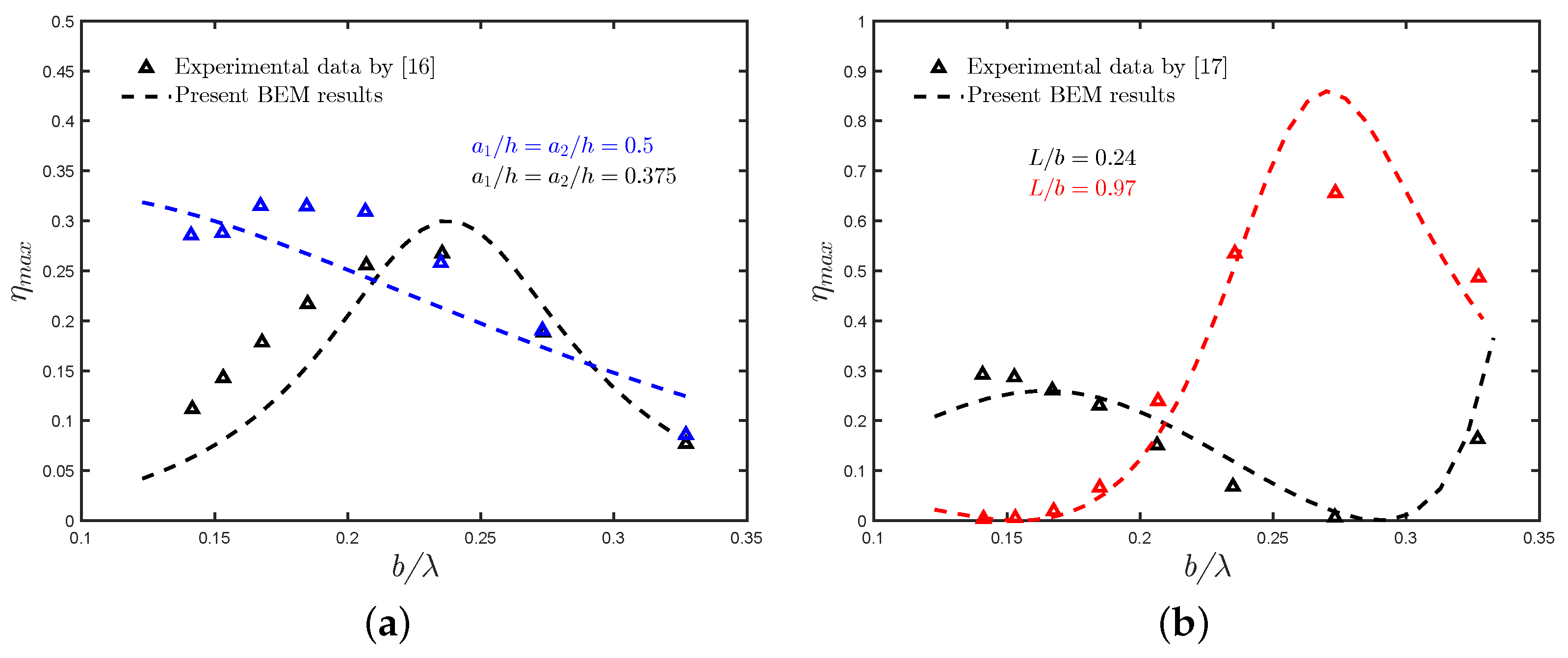
6. Comparison with Experimental Results

To validate the results obtained by the above-mentioned methods, the experimental results of [16,17] were employed. In Figure 4a, comparisons are shown of the experimental data of [16] and the present BEM results for the hydrodynamic efficiency versus $b/\lambda$ with $b/h=1.0$ and $w_1/h=w_2/h=0.025$ for two different values of the walls draft to water depth ratio $a_1/h=a_2/h$. The damping coefficients for these results were $\mathsf{\Lambda }=0.008$ and $\mathsf{\Lambda }=0.00005$ m${}^4·$s/kg for $a_1/h=a_2/h=0.375$ and $a_1/h=a_2/h=0.50$, respectively. To determine the damping coefficient $\mathsf{\Lambda }$, the method described by [41] was employed. The ratios of slot opening to cross-sectional area of the OWC chamber considered by [16] were 0.625% and 1.875% for $a_1/h=a_2/h$ equal to 0.5 and 0.375, respectively. In Figure 4b, the hydrodynamic efficiency versus $b/\lambda$ with $b/h=1.0$, $a_1/h=a_2/h=0.25$ and $w_1/h=w_2/h=0.025$ for two different values of the rear face to reflecting wall distance to chamber length ratio $L/b$ is compared against the results obtained by [17]. In this case, the damping coefficients were $\mathsf{\Lambda }=0.0018$ and $\mathsf{\Lambda }=0.0030$ m${}^4·$s/kg for $L/b=0.24$ and $L/b=0.97$, respectively. Here, the opening ratio considered by [17] was 1.25% in both cases.

From these figures, it can be seen that the BEM results follow a similar trend to that observed in the experimental data. However, for the case of the highest draft $a_1/h=a_2/h=0.5$ with the smallest opening ratio, $0.625\%$, as is the case of the PTO mechanism in [16], the difference is more significant. This discrepancy obtained with the present results arises from the assumption of an ideal fluid, where viscous effects and flow separation due to the OWC structure are ignored. This also leads to an overestimation of the hydrodynamic performance. Other factors that also contribute to the discrepancy are the modelled PTO system, as well as the energy loss through it by viscous dissipation during the tests.

7. Results and Discussion

Analytical and numerical results based on the previously described methodologies are provided in this section. The influence of the rear and front wall thickness to water depth ratio $(w_1/h,w_2/h)$, the chamber length to water depth ratio $(b/h)$, the rear and front walls draft to water depth ratio $(a_1/h,a_2/h)$, the step height to water depth ratio $(h_e/h)$ and the chamber to wall distance to water depth ratio $(L/h)$ on the hydrodynamic performance are analyzed.

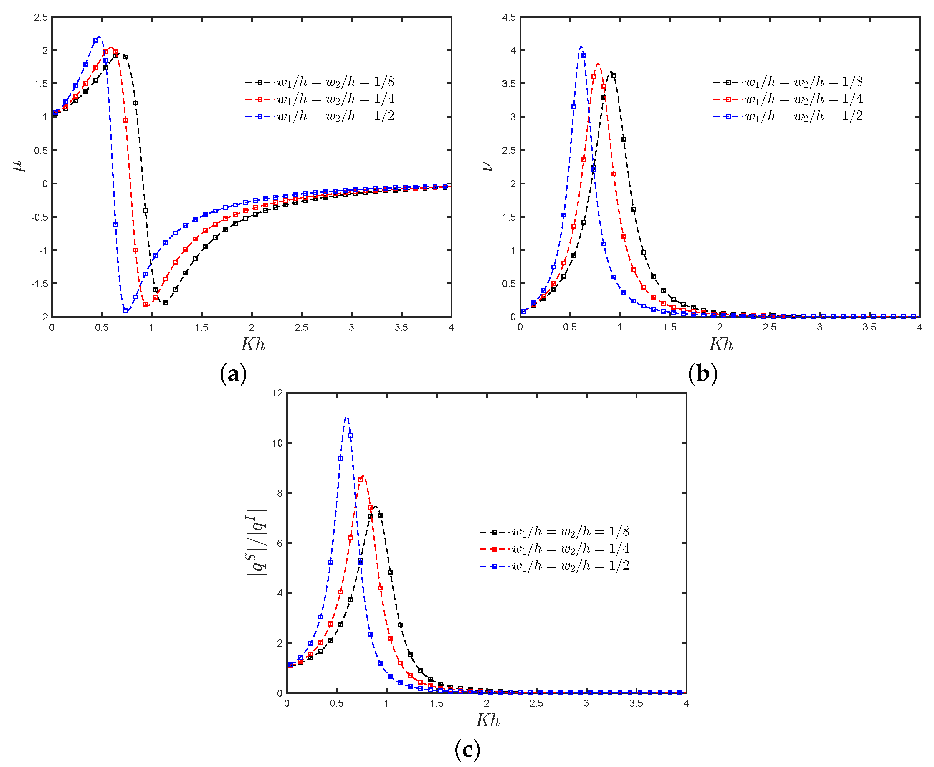
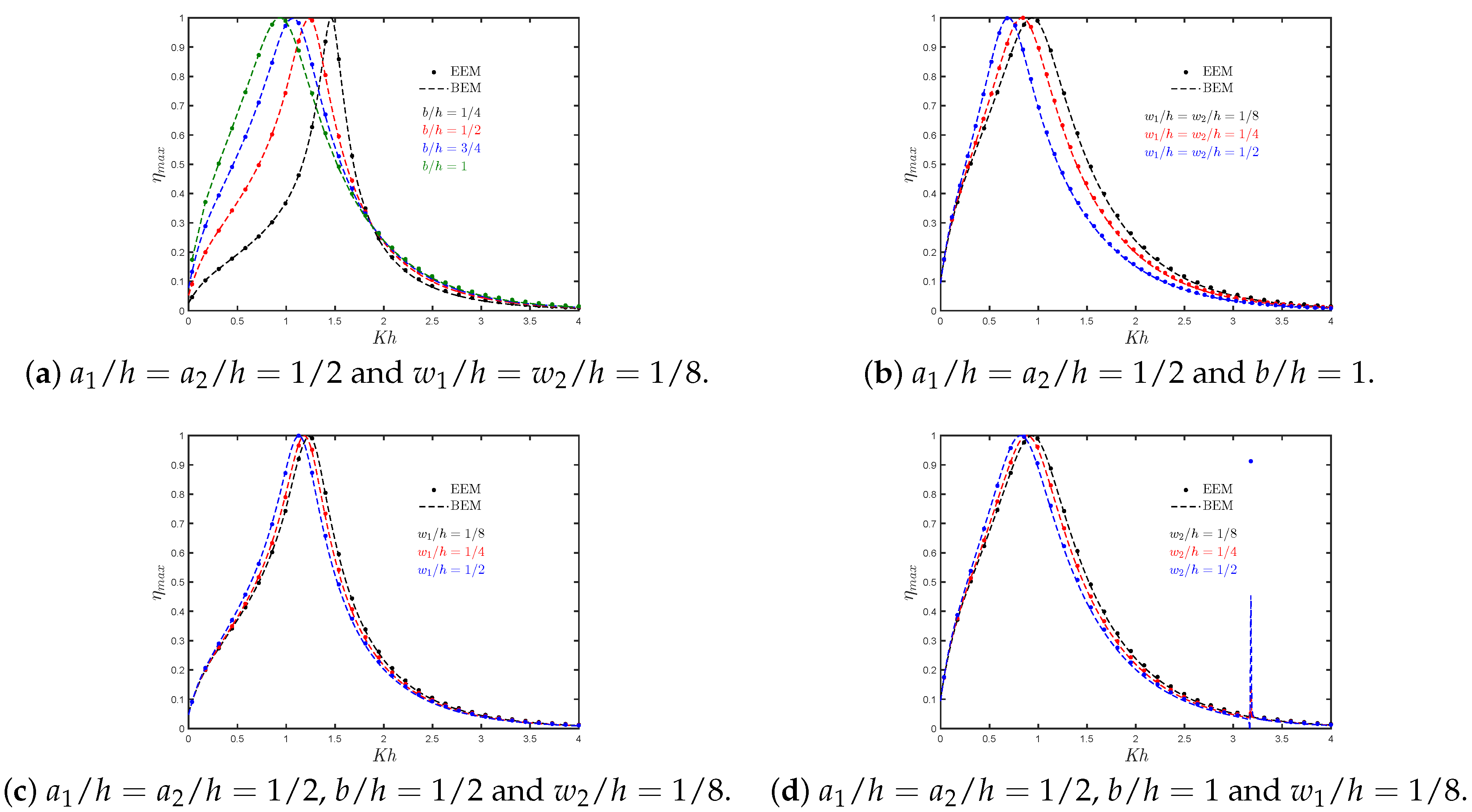
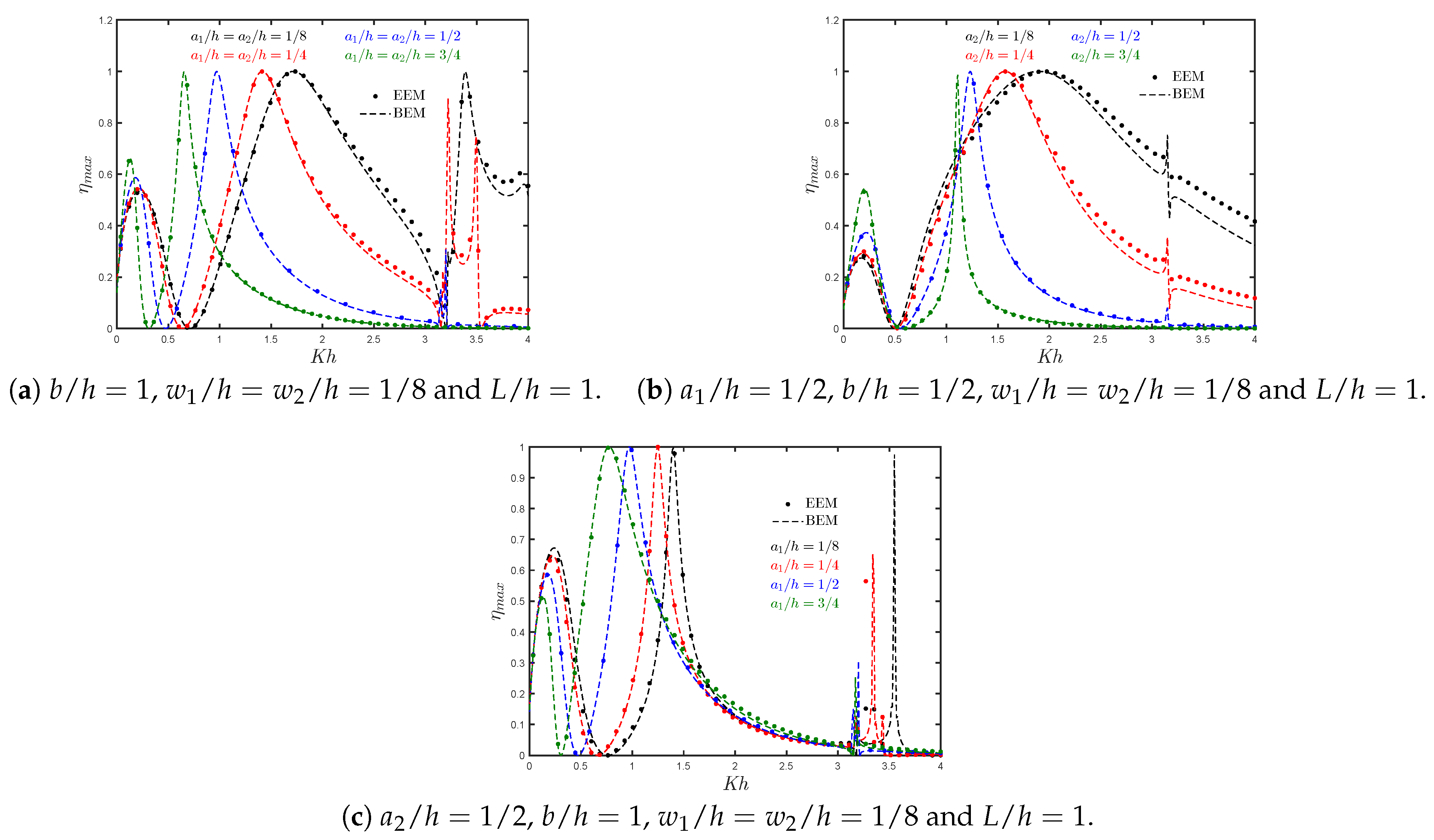
7.1. Asymmetric Fixed-Detached OWC Device over a Flat Bottom

The theoretical results of the hydrodynamic efficiency ${\eta }_{max}$ versus $Kh$ for different chamber lengths $b/h(=1/4,1/2,3/4,\mathrm{and}1)$ are shown in Figure 5a. It can be seen in this figure that increasing the length of the chamber increases the bandwidth of the efficiency curves. In this regard, large motions occur in the internal water column when the fluid is excited into a resonant piston-like motion by the incident wave [9]. The natural frequency of oscillation can be calculated for small values of the $b/h$ ratio, allowing the water enclosed within the chamber to be treated as a solid body. By simple hydrostatic modelling, it results that the expected resonance occurs at $Kh\approx h/a_1$. For the cases shown in Figure 5a, this resonance would occur at $Kh=2$, which appears to be approached for small $b/h$. Furthermore, it is observed that for large $b/h$ ratios, the peak frequency value is shifted to lower frequencies. This is because increasing the chamber length increases the horizontal distance a fluid particle must travel during a period of motion, resulting in a reduction in the value at which resonance occurs. Furthermore, since a longer chamber allows for a greater local fluid motion, the solid-body concept of resonance breaks down, and the oscillation amplitude decreases [9].

The results of the hydrodynamic efficiency versus the non-dimensional frequency $Kh$ for different thickness ratios of the front and rear walls $w_1/h=w_2/h(=1/8,1/4,\mathrm{and}1/2)$ are shown in Figure 5b. This figure shows that the bandwidth of the efficiency curves is reduced as the thickness of the walls is increased, and their peak frequency value is moved to lower values of the non-dimensional frequency $Kh$. This drop in efficiency at medium and high frequencies can be explained by the fact that the energy transfer due to wave motion for relatively small wavelengths decreases as wall thickness increases. On the other hand, Figure 5c,d shows the variation of ${\eta }_{max}$ versus $Kh$ for different thicknesses of the rear and front walls, respectively. Similar to Figure 5b, in these figures it is observed that the bandwidth of the efficiency and the peak frequency magnitude decrease when the thickness of the front or rear walls increases. Furthermore, a second resonance peak that occurs when conditions are similar to those in a closed tank with parallel walls is observed in Figure 5d. In such conditions, the incidence wave frequency is such that the fluid in the chamber is excited in an anti-symmetric sloshing mode [9]. In this case, the sloshing frequencies are seen to occur at values of the dimensionless wavenumber $kb=n\pi$, with n being the sloshing mode. Thus, the second peaks in ${\eta }_{max}$ caused by the first sloshing frequency occur at $Kh\approx \pi$ for $b/h=1$.

Figure 6a shows the effect on the efficiency of different submergence ratios $a_1/h=a_2/h(=1/8,1/4,1/2,\mathrm{and}3/4)$ versus $Kh$. This figure shows that the effective area under the efficiency curve and the magnitude of the natural frequency both increase when the walls submergence ratio $a_1/h$ and $a_2/h$ decreases. However, while a small draft results in a better performance for a wider frequency range, in practice, tidal fluctuations and extreme waves may compromise its effectiveness since a small draft may mean that the trough of a wave propagates below the front wall. In this instance, the pressure inside the chamber would be equivalent to the ambient pressure, resulting in no power available within the OWC device. Furthermore, Figure 6b,c shows the variation of ${\eta }_{max}$ versus $Kh$ for an asymmetric OWC device with different drafts of the front and rear walls, respectively. As in Figure 6a, these figures show that the bandwidth of the efficiency and the peak frequency magnitude decrease when the submergence of the front or rear walls increase. Additionally, in Figure 6b a second resonance mechanism due to the first sloshing frequency at $Kh\approx \pi$ for $b/h=1$ is observed.

Figure 7a–c shows the analytical results for the radiation susceptance and radiation conductance coefficients, $\mu$ and $\nu$, respectively, and the non-dimensional induced volume flux due to the scattering potential $|q^S|/|q^I|$ versus $Kh$ for different values of $b/h(=1/4,1/2,3/4,\mathrm{and}1)$. Figure 7a shows that the peak and the range of positive values in the radiation susceptance coefficient increase when chamber length increases. From Figure 7b it is observed that the bandwidth in the radiation conductance curves decreases as $b/h$ increases, similar to the trend observed in ${\eta }_{max}$, see Figure 5a. Moreover, the zero values in $\mu$ are associated with the peak values in $\nu$, $|q^S|/|q^I|$, Figure 7c, and ${\eta }_{max}$, due to the fundamental resonance inside the chamber.

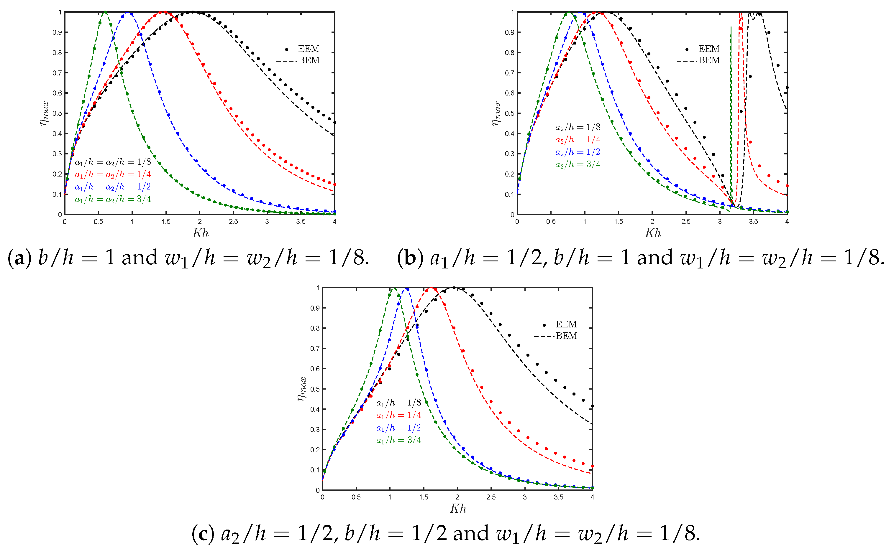
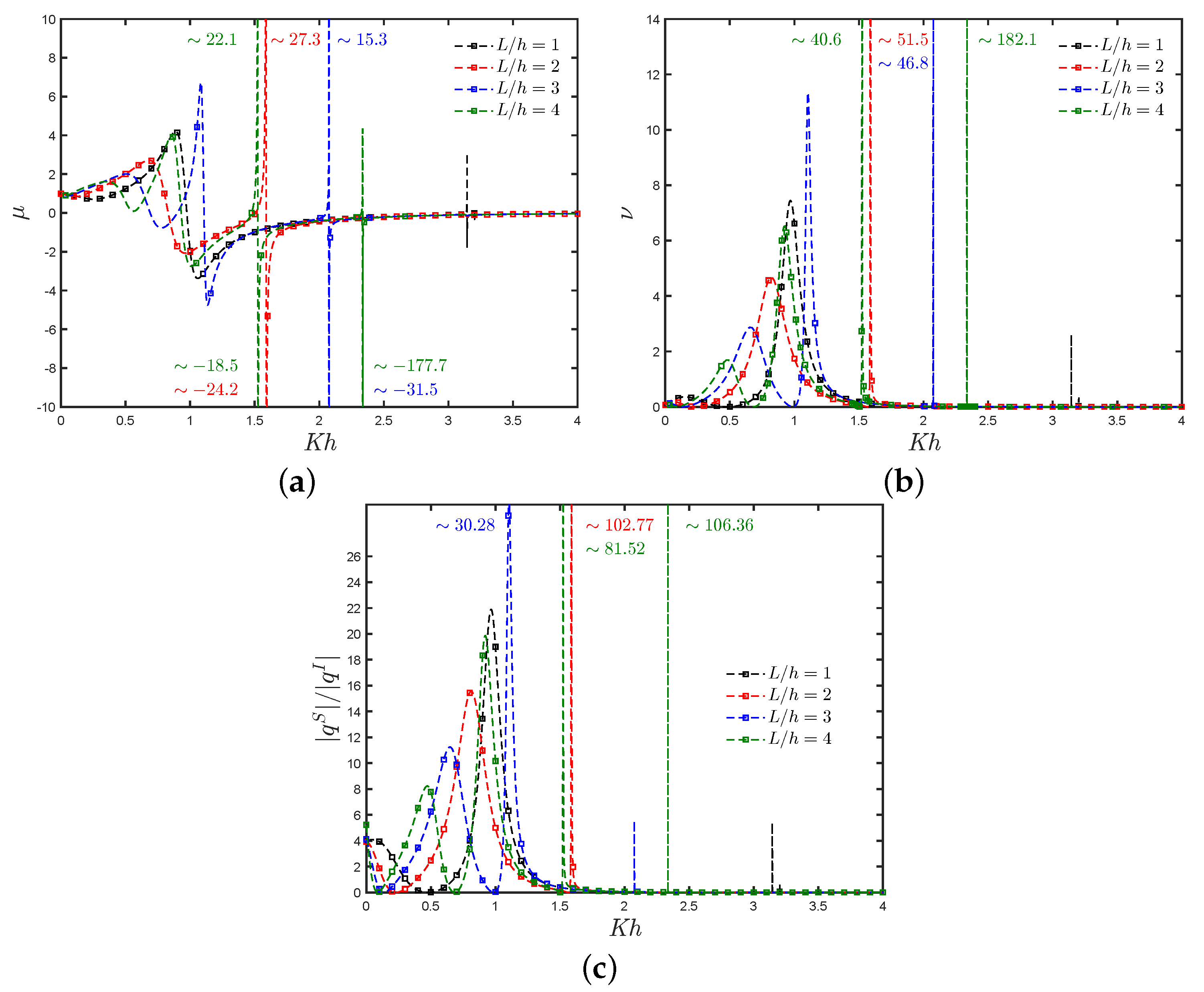
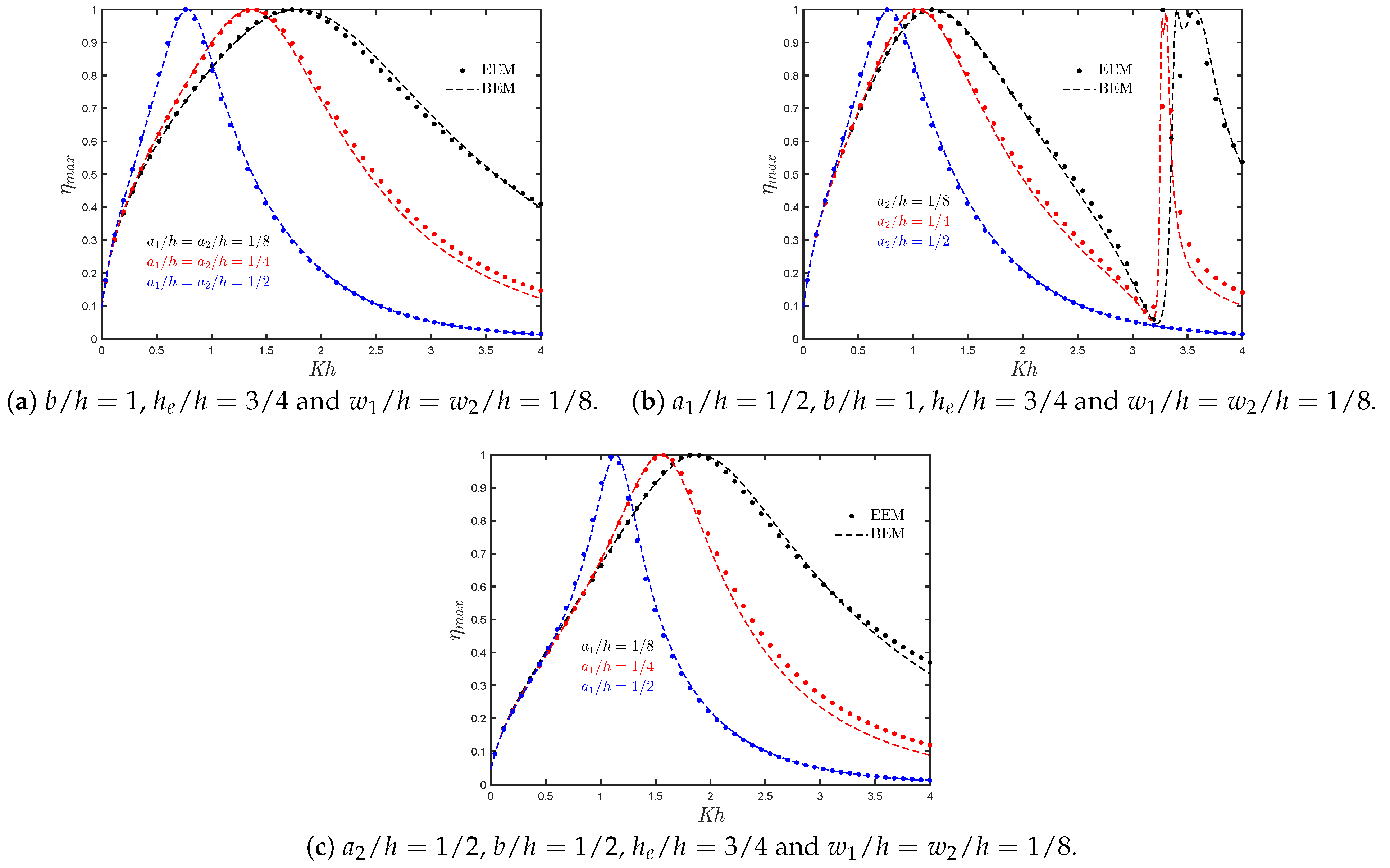
7.2. Asymmetric Fixed-Detached OWC Device over a Step

Figure 8a shows the analytical and numerical results of the hydrodynamic efficiency ${\eta }_{max}$ versus $Kh$ for different chamber lengths to water depth ratios $b/h(=1/4,1/2,3/4,\mathrm{and}1)$. This figure shows that the value of the resonance peak frequency decreases when the length of the chamber increases and, compared to the case when $h_e/h=1$ (Figure 5a), it is observed that the step contributes to a reduction in the value of $Kh$ at which resonance occurs.

Figure 8b shows the theoretical results of the hydrodynamic efficiency versus the non-dimensional frequency $Kh$ for different thickness ratios of the front and rear walls $w_1/h=w_2/h(=1/8,1/4,\mathrm{and}1/2)$. In this case, it is seen that a reduction in the bandwidth of the efficiency curves is obtained when the thickness of the walls increases. Moreover, it is also observed that the magnitude of the resonance frequency $Kh$ is reduced since, for a large thickness, longer waves are needed to excite the internal water column. On the other hand, the variation of ${\eta }_{max}$ versus $Kh$ for different thicknesses of the rear and front walls are shown in Figure 8c,d, respectively. Again, it is observed that whether the thickness of the rear or front wall increases, the resonance frequency $Kh$ is reduced.

The effects of different submergence ratios $a_1/h=a_2/h(=1/8,1/4,\mathrm{and}1/2)$ on the efficiency versus $Kh$ are shown in Figure 9a. It is observed that performance for higher frequencies increases when the submergence ratio $a_1/h$ and $a_2/h$ decreases in the rear and front walls, respectively. Compared to Figure 6a where a flat bottom is considered, in this case, the value of the peak frequency is slightly decreased since the gap between the lip of the walls and the bottom is reduced. On the other hand, the variations of ${\eta }_{max}$ versus $Kh$ for different drafts of the front and rear walls are shown in Figure 9b,c, respectively. These figures show that the hydrodynamic performance is sensitive to variations in the draft of the walls, reducing its magnitude for high frequencies as the submergence increases. In Figure 9b it is also observed a second resonance mechanism at $Kh\approx \pi$ as in Figure 6b, while in Figure 9c this will take place at $Kh\approx 2\pi$ since $b/h=1/2$.

Figure 10a–c shows the analytical results for the radiation susceptance and radiation conductance coefficients, $\mu$ and $\nu$, respectively, and the non-dimensional induced volume flux due to the scattering potential $|q^S|/|q^I|$ versus $Kh$ for different values of $w_1/h=w_2/h(=1/8,1/4,\mathrm{and}1/2)$. In Figure 10a it is observed the peak in $\mu$ increases when the thickness in the walls also increases, while the peak shifts to the lower-frequency side. However, it is observed that the range of negative values increases as the thickness increases. Figure 10b shows that the curve in the radiation conductance coefficient becomes sharper as the thickness increases, which indicates a reduction in the frequency range for the energy transfer into the system. A decreasing trend in the peak of the non-dimensional induced volume flux due to the scattering potential when the thickness decreases is observed in Figure 10c.

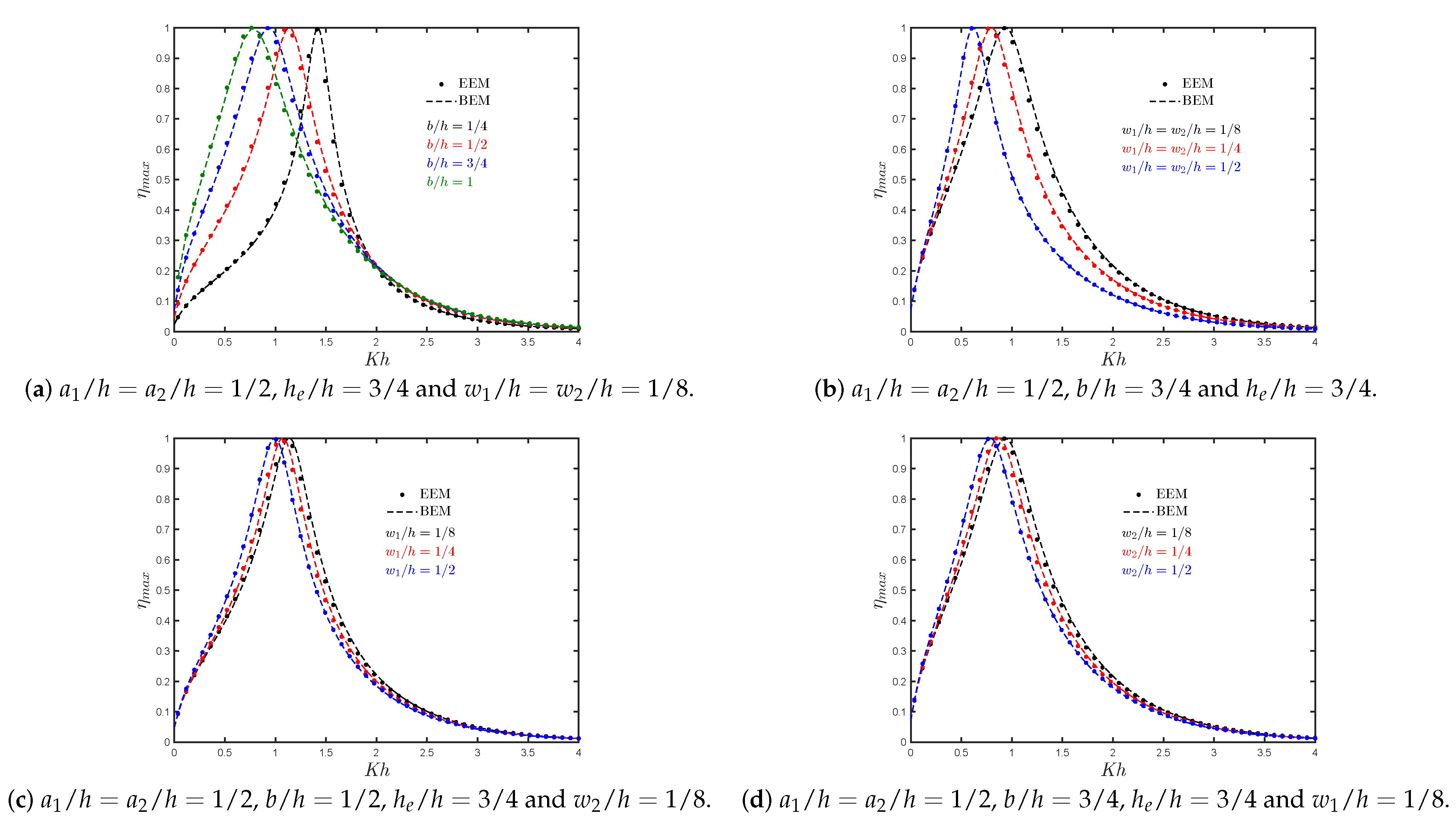
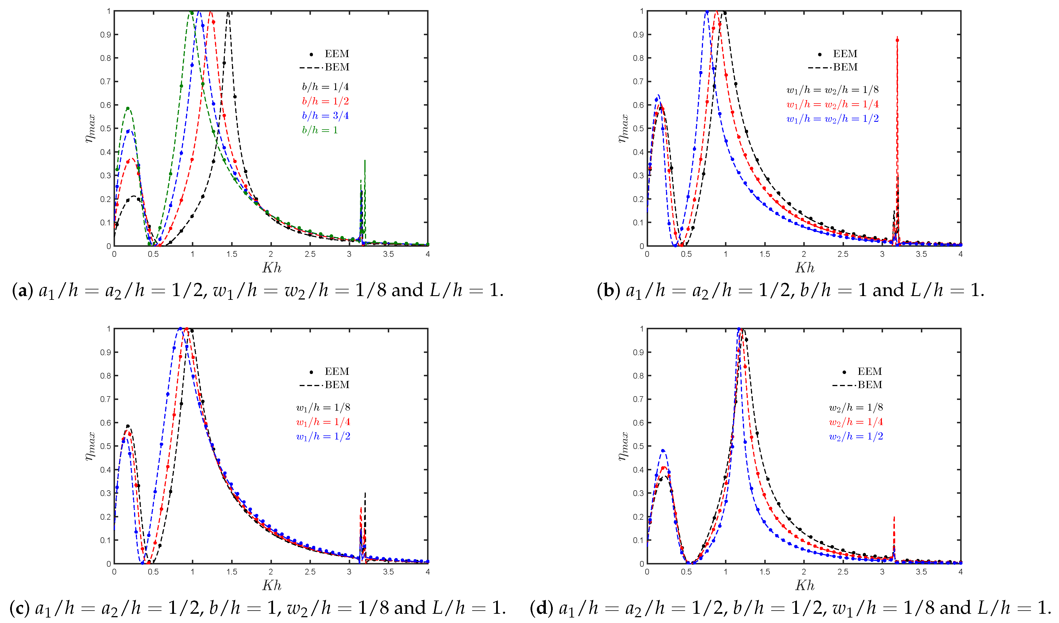
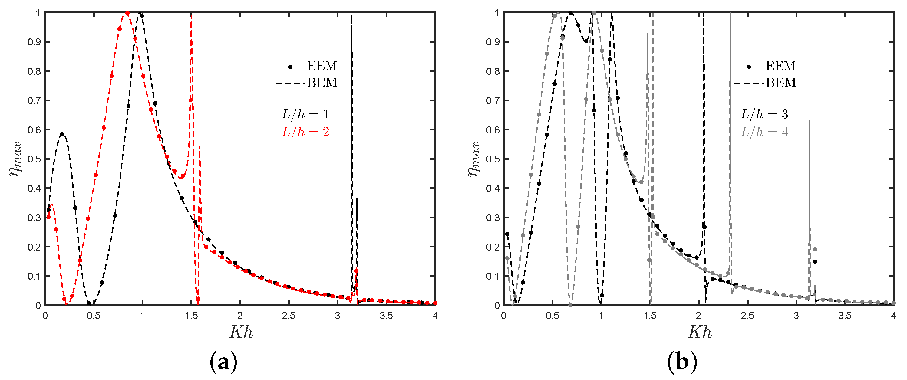
7.3. Asymmetric Fixed-Detached OWC Device near a Reflecting Wall

The analytical and numerical results of the hydrodynamic efficiency ${\eta }_{max}$ versus $Kh$ for an OWC device in the presence of a reflection wall with different chamber length to water depth ratios $b/h(=1/4,1/2,3/4,\mathrm{and}1)$ are shown in Figure 11a. Compared to Figure 5a, it is observed that the efficiency bandwidth is reduced when a reflecting wall is considered. In this case, it is observed that due to the near trapped waves in the gap between the OWC chamber and the rigid vertical wall, a medium-height peak at low frequencies appears in the efficiency curves. This peak increases as the chamber length to water depth ratio increases. Furthermore, a zero efficiency value appears at 0.45$<Kh<$0.61 that reduces the possibility of wave energy extraction at large periods.

The results of the hydrodynamic efficiency versus $Kh$ for various thickness ratios $w_1/h=w_2/h(=1/8,1/4,\mathrm{and}1/2)$ are shown in Figure 11b. It is observed that an increase in the thickness of the walls leads to both reduction of the bandwidth of the efficiency curves and the peak frequency value. Furthermore, it is seen that when $w_1/h$ and $w_2/h$ increase, the medium-height peak slightly increases, while the zero efficiency value is shifted to lower frequencies.

Figure 11c shows that with an increase in the rear wall thickness, the medium-height peak at low frequencies and the resonant frequency value of maximum efficiency both decrease. On the other hand, in Figure 11d for $b/h=1/2$, it is observed that the bandwidth of the efficiency curves is highly reduced, and the medium-height peak is increased when the front wall thickness increases. Furthermore, Figure 6a–d shows a second resonance mechanism due to the first sloshing frequency at $Kh\approx \pi$.

The effect of different draft ratios $a_1/h=a_2/h(=1/8,1/4,\mathrm{and}1/2)$ on the efficiency versus $Kh$ for a symmetric OWC device is shown in Figure 12a. It is observed that the peak resonant frequency and the efficiency bandwidth are significantly reduced when the ratios $a_1/h$ and $a_2/h$ increase. Furthermore, the frequency value of zero efficiency increases and the peak at low frequencies decreases when the submergence in the front and rear walls decreases.

The variations of maximum efficiency ${\eta }_{max}$ versus the non-dimensional frequency $Kh$ for different drafts of the rear and front walls are shown in Figure 12b,c, respectively. In both of them, it is observed that by increasing the submergence of one of the walls, the values of the frequency at which resonance occurs are decreased. However, in Figure 12b, the efficiency bandwidth is increased when the submergence of the front wall decreases, while the peak at low frequencies decreases. On the other hand, in terms of the medium-height peak, Figure 12c shows an opposite trend to that observed in Figure 12b.

The results of the hydrodynamic efficiency versus the non-dimensional frequency $Kh$ for different lengths of the gap between the rear and reflecting walls $L/h(=1,2,3,\mathrm{and}4)$ are shown in Figure 13a,b. In these two figures, it is observed that the bandwidth of the efficiency increases, while the medium-height peak at low frequencies reduces when the distance of separation between the fixed OWC and the reflecting wall increases. It is also observed that at $L/h=3$ and 4, the shape of the curve tend to that observed in Figure 5a for $b/h=1$, although a peaky trend is observed for $L/h=4$. All these aspects should be considered at the design stage since the near trapped waves generated between the reflecting wall and the OWC device can reduce the efficiency bandwidth of a fixed-detached OWC device at high periods.

The analytical results for the radiation susceptance and radiation conductance coefficients, $\mu$ and $\nu$, respectively, and the non-dimensional induced volume flux due to the scattering potential $|q^S|/|q^I|$ versus the non-dimensional frequency $Kh$ for different values of $L/h(=1,2,3,\mathrm{and}4)$ are shown in Figure 14a–c. Figure 14a shows a decrease in the negative values of $\mu$ when the gap between the rear and reflecting walls also decreases. As in [10], in Figure 14a,b it is observed that at resonance, the total variation from positive to negative in the radiation susceptance coefficient is related to the peak values of the radiation conductance. Finally, from Figure 14b,c it is observed that the peak in $\nu$ and $|q^S|/|q^I|$, respectively, at the fundamental resonance increase when $L/h$ decrease.

8. Conclusions

The influence of the geometric parameters of an asymmetric fixed-detached OWC device on the hydrodynamic efficiency was theoretically analyzed. The BEM with quadratic elements and the matched EEM were employed to solve the radiation and scattering problems. Comparisons were made between these two methods and a good agreement was obtained. A comparison was made between the experimental data of [16,17] giving a satisfactory agreement. Results for different hydrodynamic quantities of interest were then obtained for different physical configurations. The main conclusions of this study are as follows:

• An increase in the chamber length leads to an increase in the bandwidth of the efficiency curves. This is similar to the findings for a land-fixed OWC device reported by Evans and Porter [9].
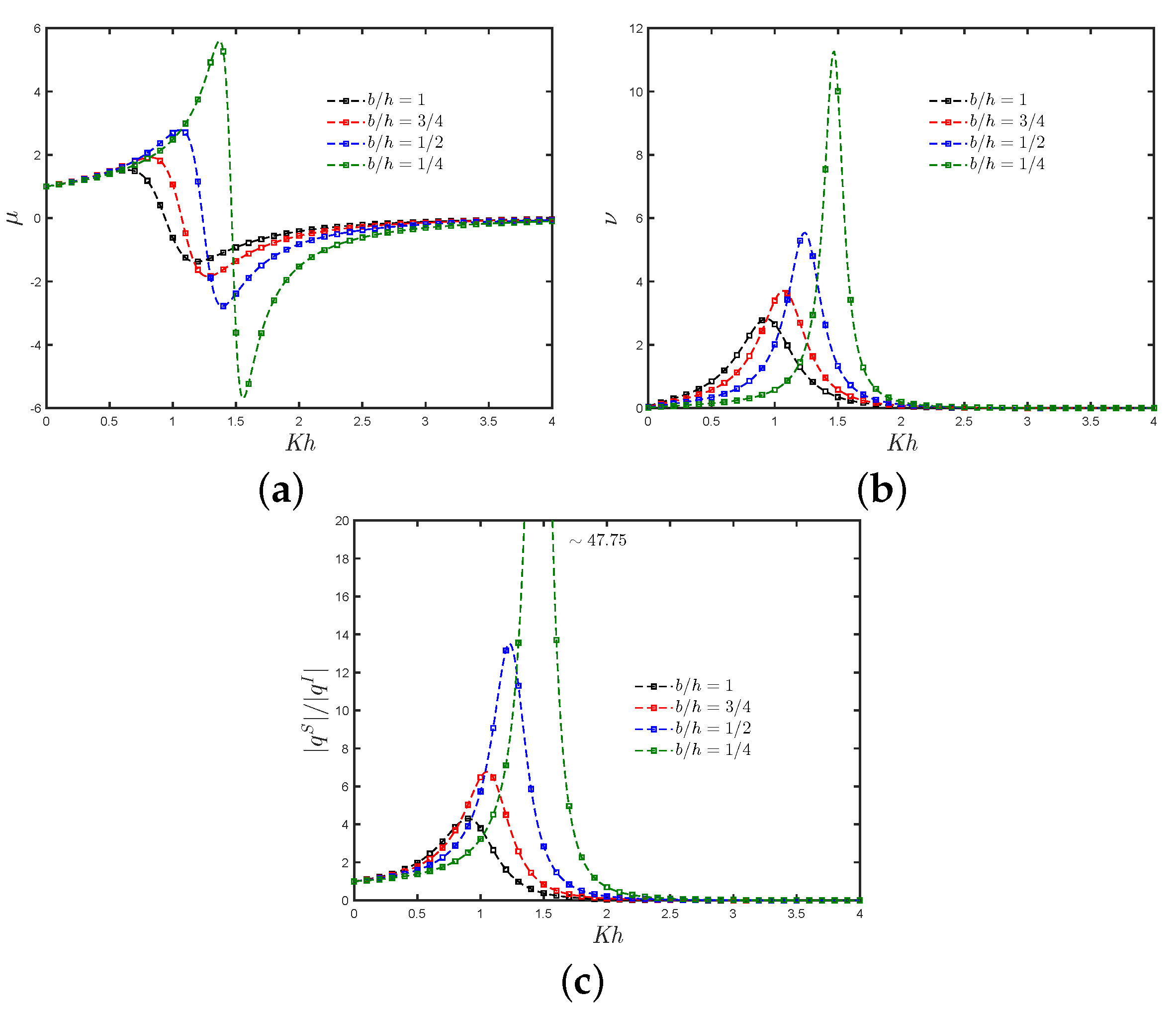
• By increasing the thickness of the rear and front walls, the bandwidth of the efficiency curves and their peak frequency value are reduced. This reduction in efficiency, especially for short wavelengths, is due to the decrease in energy transfer owing to the wave motion when a large thickness is considered.
• Both the effective area under the efficiency curves and the magnitude of the natural frequency increase when the submergence of the walls decreases. This is because a larger gap between the front wall lip and the bottom allows more energy to be transferred to the water column.
• Regarding the presence of a step, it was observed that this reduces the frequency at which resonance occurs since the effect is similar to reducing the gap between the lip of the walls and the bottom.
• When the separation distance is shorter, the near trapped and standing waves in the gap of the OWC chamber and the reflecting wall play a significant role in the hydrodynamic performance. It was observed that the efficiency bandwidth is reduced, and a medium-height peak appears at low frequencies.
• At low frequencies, the presence of constructive and destructive wave interference from the OWC device and the waves reflected by the wall results in zero efficiency. This phenomenon is extremely sensitive to changes in the OWC parameters, and engineers should take it into account when constructing a fixed-detached OWC device near a vertical wall.

Finally, this work is only a theoretical investigation of the hydrodynamic performance of a fixed-detached OWC device. The construction of a fixed-detached OWC device near a rigid vertical wall may constitute an alternative for reducing the wave load on seawalls by absorbing the incident wave energy and can be extended to include an array of fixed-detached OWC devices. Numerical simulations and experimental tests of other geometrical conditions and non-linearities on the air compressibility and turbine damping due to viscous effects should be carried out in the future to improve the present results.

References

1. Gunn, K.; Stock-Williams, C. Quantifying the global wave power resource. Renew. Energy 2012, 44, 296–304. [Google Scholar] [CrossRef]
2. Calheiros-Cabral, T.; Clemente, D.; Rosa-Santos, P.; Taveira-Pinto, F.; Ramos, V.; Morais, T.; Cestaro, H. Evaluation of the annual electricity production of a hybrid breakwater-integrated wave energy converter. Energy 2020, 213, 118845. [Google Scholar] [CrossRef]
3. Falcão, A.F.O. Wave energy utilization: A review of the technologies. Renew. Sustain. Energy Rev. 2010, 14, 899–918. [Google Scholar] [CrossRef]
4. Falcão, A.F.O.; Henriques, J.C.C. Oscillating-water-column wave energy converters and air turbines: A review. Renew. Energy 2016, 85, 1391–1424. [Google Scholar] [CrossRef]
5. Falnes, J.; McIver, P. Surface wave interactions with systems of oscillating bodies and pressure distributions. Appl. Ocean Res. 1985, 7, 225–234. [Google Scholar] [CrossRef]
6. Evans, D.V. A theory for wave-power absorption by oscillating bodies. J. Fluid Mech. 1976, 77, 1–25. [Google Scholar] [CrossRef]
7. Evans, D.V. Power from water waves. Annu. Rev. Fluid Mech. 1981, 13, 157–187. [Google Scholar] [CrossRef]
8. Mei, C.C. Power Extraction from Water Waves. J. Mar. Res. 1976, 20, 63–66. [Google Scholar]
9. Evans, D.; Porter, R. Hydrodynamic characteristics of an oscillating water column device. Appl. Ocean Res. 1995, 17, 155–164. [Google Scholar] [CrossRef]
10. Evans, D.; Porter, R. Efficient calculation of hydrodynamic properties of owc-type devices. ASME. J. Offshore Mech. Arct. Eng. 1997, 119, 210–218. [Google Scholar] [CrossRef]
11. Şentürk, U.; Özdamar, A. Wave energy extraction by an oscillating water column with a gap on the fully submerged front wall. Appl. Ocean Res. 2012, 37, 174–182. [Google Scholar] [CrossRef]
12. Morris-Thomas, M.T.; Irvin, R.J.; Thiagarajan, K.P. An Investigation Into the Hydrodynamic Efficiency of an Oscillating Water Column. J. Offshore Mech. Arct. 2006, 129, 273–278. [Google Scholar] [CrossRef]
13. Rezanejad, K.; Bhattacharjee, J.; Guedes Soares, C. Stepped sea bottom effects on the efficiency of nearshore oscillating water column device. Ocean Eng. 2013, 70, 25–38. [Google Scholar] [CrossRef]
14. Wang, D.J.; Katory, M.; Li, Y.S. Analytical and experimental investigation on the hydrodynamic performance of onshore wave-power devices. Ocean Eng. 2002, 29, 871–885. [Google Scholar] [CrossRef]
15. Sarmento, A.J.N.A. Wave flume experiments on two-dimensional oscillating water column wave energy devices. Exp. Fluids 1992, 12, 286–292. [Google Scholar] [CrossRef]
16. He, F.; Li, M.; Huang, Z. An Experimental Study of Pile-Supported OWC-Type Breakwaters: Energy Extraction and Vortex-Induced Energy Loss. Energies 2016, 9, 540. [Google Scholar] [CrossRef] [Green Version]
17. He, G.; Huang, Z. Using an Oscillating Water Column Structure to Reduce Wave Reflection from a Vertical Wall. J. Waterw. Port Coast. Ocean Eng. 2016, 142, 04015021. [Google Scholar] [CrossRef]
18. He, F.; Zhang, H.; Zhao, J.; Zheng, S.; Iglesias, G. Hydrodynamic performance of a pile-supported OWC breakwater: An analytical study. Appl. Ocean Res. 2019, 88, 326–340. [Google Scholar] [CrossRef]
19. Karthik, S.; Sundar, V.; Sannasiraj, S.A. Hydrodynamic performance characteristics of an oscillating water column device integrated with a pile breakwater. J. Ocean Eng. Mar. Energy 2021, 7, 229–241. [Google Scholar] [CrossRef]
20. Iturrioz, A.; Guanche, R.; Armesto, J.A.; Alves, M.A.; Vidal, C.; Losada, I.J. Time-domain modeling of a fixed detached oscillating water column towards a floating multi-chamber device. Ocean Eng. 2014, 76, 65–74. [Google Scholar] [CrossRef]
21. Iturrioz, A.; Guanche, R.; Lara, J.L.; Vidal, C.; Losada, I.J. Validation of OpenFOAM® for Oscillating Water Column three-dimensional modeling. Ocean Eng. 2015, 107, 222–236. [Google Scholar] [CrossRef]
22. Simonetti, I.; Cappietti, L.; Elsafti, H.; Oumeraci, H. Optimization of the geometry and the turbine induced damping for fixed detached and asymmetric OWC devices: A numerical study. Energy 2017, 139, 1197–1209. [Google Scholar] [CrossRef]
23. Qu, M.; Yu, D.Y.; Dou, Z.H.; Wang, S.L. Design and Experimental Study of A Pile-Based Breakwater Integrated with OWC Chamber. China Ocean Eng. 2021, 35, 443–453. [Google Scholar] [CrossRef]
24. Elhanafi, A.; Macfarlane, G.; Fleming, A.; Leong, Z. Investigations on 3D effects and correlation between wave height and lip submergence of an offshore stationary OWC wave energy converter. Appl. Ocean Res. 2017, 64, 203–216. [Google Scholar] [CrossRef]
25. Elhanafi, A.; Fleming, A.; Macfarlane, G.; Leong, Z. Underwater geometrical impact on the hydrodynamic performance of an offshore oscillating water column–wave energy converter. Renew. Energy 2017, 105, 209–231. [Google Scholar] [CrossRef]
26. Elhanafi, A.; Fleming, A.; Macfarlane, G.; Leong, Z. Numerical hydrodynamic analysis of an offshore stationary–floating oscillating water column–wave energy converter using CFD. Int. J. Nav. Archit. 2017, 9, 77–99. [Google Scholar] [CrossRef] [Green Version]
27. Elhanafi, A.; Kim, C.J. Experimental and numerical investigation on wave height and power take–off damping effects on the hydrodynamic performance of an offshore–stationary OWC wave energy converter. Renew. Energy 2018, 125, 518–528. [Google Scholar] [CrossRef]
28. Zabihi, M.; Mazaheri, S.; Montazeri-Namin, M. Experimental hydrodynamic investigation of a fixed offshore Oscillating Water Column device. Appl. Ocean Res. 2019, 85, 20–33. [Google Scholar] [CrossRef]
29. Michele, S.; Renzi, E.; Perez-Collazo, C.; Greaves, D.; Iglesias, G. Power extraction in regular and random waves from an OWC in hybrid wind-wave energy systems. Ocean Eng. 2019, 191, 106519. [Google Scholar] [CrossRef]
30. Deng, Z.; Wang, C.; Wang, P.; Higuera, P.; Wang, R. Hydrodynamic performance of an offshore-stationary OWC device with a horizontal bottom plate: Experimental and numerical study. Energy 2019, 187, 115941. [Google Scholar] [CrossRef]
31. Deng, Z.; Ou, Z.; Ren, X.; Zhang, D.; Si, Y. Theoretical Analysis of an Asymmetric Offshore-Stationary Oscillating Water Column Device with Bottom Plate. J. Waterw. Port Coast. Ocean Eng. 2020, 146, 04020013. [Google Scholar] [CrossRef]
32. Medina-Lopez, E.; Allsop, W.; Dimakopoulos, A.; Bruce, T. Conjectures on the Failure of the OWC Breakwater at Mutriku. In Proceedings of the Coastal Structures and Solutions to Coastal Disasters Joint Conference, Boston, MA, USA, 9–11 September 2015. [Google Scholar]
33. Evans, D.V. Wave-power absorption by systems of oscillating surface pressure distributions. J. Fluid Mech. 1982, 114, 481–499. [Google Scholar] [CrossRef]
34. Katsikadelis, J. Boundary Elements. Theory and Applications; Elsevier: Amsterdam, The Netherlands, 2002. [Google Scholar]
35. Medina Rodríguez, A.A.; Blanco Ilzarbe, J.M.; Silva Casarín, R.; Izquierdo Ereño, U. The Influence of the Chamber Configuration on the Hydrodynamic Efficiency of Oscillating Water Column Devices. J. Mar. Sci. Eng. 2020, 8, 751. [Google Scholar] [CrossRef]
36. Dominguez, J. Boundary Elements in Dynamics; Computational Mechanics Publications: Southampton, UK, 1993. [Google Scholar]
37. Medina Rodríguez, A.A.; Martínez Flores, A.; Blanco Ilzarbe, J.M.; Silva Casarín, R. Interaction of oblique waves with an Oscillating Water Column device. Ocean Eng. 2021, 228, 108931. [Google Scholar] [CrossRef]
38. Becker, A. The Boundary Element Method in Engineering: A Complete Course; McGraw-Hill Book Company: London, UK, 1992. [Google Scholar]
39. Falcão, A.F.O.; Henriques, J.C.C.; Cândido, J.J. Dynamics and optimization of the OWC spar buoy wave energy converter. Renew. Energy 2012, 48, 369–381. [Google Scholar] [CrossRef]
40. Gato, L.M.C.; Falcão, A.F.O. Aerodynamics of the wells turbine. Int. J. Mech. Sci. 1988, 30, 383–395. [Google Scholar] [CrossRef]
41. Rezanejad, K; Soares, C.G.; López, I.; Carballo, R. Experimental and numerical investigation of the hydrodynamic performance of an oscillating water column wave energy converter. Renew. Energy 2017, 106, 1–16. [Google Scholar] [CrossRef]
Figure 1. Side view of the interaction of a fixed-detached OWC device with water waves.
Water 13 02637 g001
Figure 2. Side view of the interaction of water waves with a fixed-detached OWC device near a vertical wall.
Water 13 02637 g002
Figure 3. Meshing and matching of the regions with nodes arranged in an anti-clockwise direction.
Water 13 02637 g003
Figure 4. Comparison of the present results for the hydrodynamic efficiency η m a x with the experimental results obtained by (a) [16] for a pile-supported OWC device and (b) [17] for an OWC device near a reflecting vertical wall.
Water 13 02637 g004
Figure 5. Maximum hydrodynamic efficiency η m a x versus the non-dimensional frequency K h for different (a) lengths of the OWC chamber b / h ; (b) thickness of the rear and front walls, w 1 / h and w 2 / h , respectively; (c) thickness of the rear wall w 1 / h ; (d) thickness of the front wall w 2 / h .
Water 13 02637 g005
Figure 6. Maximum hydrodynamic efficiency η m a x versus the non-dimensional frequency K h for different (a) submergence depths of the rear and front walls, a 1 / h and a 2 / h , respectively; (b) submergence depths of the front wall a 2 / h ; (c) submergence depths of the rear wall a 1 / h .
Water 13 02637 g006
Figure 7. The influence of chamber length b / h on the (a) radiation susceptance coefficient, (b) radiation conductance coefficient and (c) non-dimensional induced volume flux due to the scattering potential against K h with a 1 / h = a 2 / h = 1 / 2 and w 1 / h = w 2 / h = 1 / 8 .
Water 13 02637 g007
Figure 8. Maximum hydrodynamic efficiency η m a x versus the non-dimensional frequency K h for different (a) lengths of the OWC chamber b / h ; (b) thickness of the rear and front walls, w 1 / h and w 2 / h , respectively; (c) thickness of the rear wall w 1 / h ; (d) thickness of the front wall w 2 / h .
Water 13 02637 g008
Figure 9. Maximum hydrodynamic efficiency η m a x versus the non-dimensional frequency K h for different (a) submergence depths of the rear and front walls, a 1 / h and a 2 / h , respectively; (b) submergence depths of the front wall a 2 / h ; (c) submergence depths of the rear wall a 1 / h .
Water 13 02637 g009
Figure 10. The influence of the thickness in the rear and front walls, w 1 / h and w 2 / h , respectively, on the (a) radiation susceptance coefficient, (b) radiation conductance coefficient and (c) non-dimensional induced volume flux due to the scattering potential against K h with a 1 / h = a 2 / h = 1 / 2 , b / h = 3 / 4 and h e / h = 3 / 4 .
Water 13 02637 g010
Figure 11. Maximum hydrodynamic efficiency η m a x versus the non-dimensional frequency K h for different (a) lengths of the OWC chamber b / h ; (b) thickness of the rear and front walls, w 1 / h and w 2 / h , respectively; (c) thickness of the rear wall w 1 / h ; (d) thickness of the front wall w 2 / h .
Water 13 02637 g011
Figure 12. Maximum hydrodynamic efficiency η m a x versus the non-dimensional frequency K h for different (a) submergence depths of the rear and front walls, a 1 / h and a 2 / h , respectively; (b) submergence depths of the front wall a 1 / h ; (c) submergence depths of the rear wall a 2 / h .
Water 13 02637 g012
Figure 13. The influence of the length of the gap between the rear and reflecting walls L / h on the maximum hydrodynamic efficiency η m a x versus the non-dimensional frequency K h with a 1 / h = a 2 / h = 1 / 8 , b / h = 1 and w 1 / h = w 2 / h = 1 / 8 for (a) L / h ( = 1 and 2 ) and (b) L / h ( = 3 and 4 ) .
Water 13 02637 g013
Figure 14. The influence of the length of the gap between the rear and reflecting walls L / h on the (a) radiation susceptance coefficient, (b) radiation conductance coefficient and (c) non-dimensional induced volume flux due to the scattering potential against K h with a 1 / h = a 2 / h = 1 / 8 , b / h = 1 and w 1 / h = w 2 / h = 1 / 8 .
Water 13 02637 g014