Article

A Novel Hybrid Model for Developing Groundwater Potentiality Model Using High Resolution Digital Elevation Model (DEM) Derived Factors

1
Department of Civil Engineering, College of Engineering, King Khalid University, Abha 61411, Saudi Arabia
2
Department of Geography, University of Gour Banga, Malda 732101, India
3
Department of Chemical Engineering, College of Engineering, King Khalid University, Abha 61411, Saudi Arabia
4
Department of Disaster Management, Begum Rokeya University, Rangpur 5400, Bangladesh
*
Author to whom correspondence should be addressed.
Water 2021, 13(19), 2632; https://doi.org/10.3390/w13192632
Submission received: 7 August 2021 / Revised: 18 September 2021 / Accepted: 20 September 2021 / Published: 25 September 2021
(This article belongs to the Section Hydrogeology)

Abstract

:
The present work aims to build a unique hybrid model by combining six fuzzy operator feature selection-based techniques with logistic regression (LR) for producing groundwater potential models (GPMs) utilising high resolution DEM-derived parameters in Saudi Arabia’s Bisha area. The current work focuses exclusively on the influence of DEM-derived parameters on GPMs modelling, without considering other variables. AND, OR, GAMMA 0.75, GAMMA 0.8, GAMMA 0.85, and GAMMA 0.9 are six hybrid models based on fuzzy feature selection. The GPMs were validated by using empirical and binormal receiver operating characteristic curves (ROC). An RF-based sensitivity analysis was performed in order to examine the influence of GPM settings. Six hybrid algorithms and one unique hybrid model have predicted 1835–2149 km2 as very high and 3235–4585 km2 as high groundwater potential regions. The AND model (ROCe-AUC: 0.81; ROCb-AUC: 0.804) outperformed the other models based on ROC’s area under curve (AUC). A novel hybrid model was constructed by combining six GPMs (considering as variables) with the LR model. The AUC of ROCe and ROCb revealed that the novel hybrid model outperformed existing fuzzy-based GPMs (ROCe: 0.866; ROCb: 0.892). With DEM-derived parameters, the present work will help to improve the effectiveness of GPMs for developing sustainable groundwater management plans.

1. Introduction

A large portion of the population all around the globe has been experiencing the problem of clean drinking water despite living on the blue Earth, mostly due to (1) the fact that only 2.5 percent of the water is drinkable; (2) the increased intake of green water (about 70% presently); and (3) the paucity of data on the possible source of groundwater on a micro-spatial level [1]. Irrigation, domestic, municipal, and industrial sectors have all increased their dependence on groundwater because it is very easily available, and it is a healthy water source [2,3]. Agriculture intensity in developing countries such as India and Bangladesh has been gradually growing in order to satisfy increasing demand for food crops. Rainfall occurs only during the monsoon season because of the region’s monsoon climate, which lasts from June to September. During non-monsoon seasons, peasants rely on groundwater for cultivation [4,5]. According to the Central Groundwater Board (CGWB, 2014), 89% of overall groundwater is harvested for irrigation, and dependence has risen unexpectedly in the urban sector [6,7,8]. India’s yearly renewable groundwater potential is estimated to be about 433 billion cubic metres (BCM), with 399 BCM of water available according to recent estimates [9,10], but the demand is several times higher than the supply. In many regions of the nation, such a scenario generally results in a decrease in the groundwater table. Furthermore, India’s groundwater generation rate is approximately 50% [9,10,11,12,13]. The Central Groundwater Board (CGWB, 2014) has compiled a list of all of the blocks in the Malda district of West Bengal, India, where groundwater production is found to be semi-critical to critical. In the midst of this crisis, it is critical to look for potential groundwater zones for raising water supply and conserving water [14,15,16].
The identifications of potential groundwater zones and the calculations of groundwater availability are essential but complex when many conditioning variables are directly and indirectly involved [17,18]. One of the best methods for this is scientific aquifer mapping, which is now almost nonexistent in most developing countries [19,20]. Geographic information systems (GIS) and remote sensing have ushered in a new era in this area, allowing multi-parametric research [14,16,21,22,23]. The choices of conditioning variables and the utilization of an efficient integration approach are crucial to effective modeling [10,24,25,26,27,28]. Table 1 shows that some groundwater potentiality modelling conditioning factors, such as soil texture, groundwater level, annual rainfall, Normalized Difference Vegetation Index (NDVI), geology, land use land cover, elevation, slope, aspect, curvature, topographic wetness index (TWI), Terrain Ruggedness Index (TRI), stream power index (SPI), distance to river, and others, have been widely used [16,21,22,29,30,31,32]. Elevation, slope, and rainfall have been identified as paramount parameters in the plains, while geology, lineament, and the other factors listed above have been identified as paramount variables in the mountainous area [24,33,34,35,36]. It is worth noting that not all of the variables are necessary for all spatial units. Drainage density, for example, may be an effective parameter in flood plains, but it may not be so in mountainous areas with several first and second order ephemeral streams. As a consequence, caution must be exercised when selecting parameters for modelling the research unit’s spatial characteristics [37].
Groundwater potential modeling is reliant on accurate data and applicable models [38]. Groundwater potentiality has been studied by using a number of methods, including physical, heuristic, and mathematical approaches [39]. Physically based methods assess groundwater potential by analyzing topographical structure and geological conditions [40,41]. Since they require very precise topography details, these methods are typically used for a small area. Depending on the experts, heuristic-based approaches determine the probability of Groundwater potentiality zones. According to Regmi et al. [42], such methods are strongly based on professional knowledge and, in general, achieve moderate precision. Groundwater potential modelling has favoured statistically based models such as statistical index (SI) [43], logistic regression (LR) [15,43], evidential belief function (EBF) [44], probability-frequency ratio (FR) [45,46], certainty factors (CF) [47,48,49], weight of evidence (WoE) [50,51], and index of entropy (IoE) [38,52] over the two groups mentioned above. These approaches are more objective and quantitative, since they are focused on existing groundwater availability areas and contributing factors. Standard statistical methods, on the other hand, are limited in their ability to predict the dynamic and nonlinear interactions between groundwater and the conditioning variables [53]. Machine learning is taken into account since no single approach or methodology is universally suitable for all fields and study area.
A vast number of groundwater-related data are becoming more readily available thanks to the rapid advancement of remote sensing technology. The majority of research used Big Data to model groundwater potentiality by using machine learning techniques since these approaches are capable of analysing the dynamic connection between groundwater potential and influencing parameters [54]. According to Jordan and Mitchell [55], machine learning is an artificial intelligence branch that employs computational algorithms to analyse and predict data by learning from training data. According to a review of the literature, artificial neural networks [56,57], neuro-fuzzy [58], decision trees [59,60], and support vector machines [44,47,61,62] have all been used to assess groundwater potential. While it is obvious that machine learning algorithms enhance prediction accuracy of regional groundwater availability, the generalisation efficiency of single classifiers also needs to be improved [63]. However, until now, groundwater researchers have been unable to agree on an appropriate model for assessing groundwater potentiality [62]. As a result, a number of ensemble methods have recently gained popularity in geohazard susceptibility and potentiality mapping [47,64,65].
The fundamental difference between the above-mentioned techniques is whether they treat data objectively or subjectively. The choice of technique is based on two factors: the analysis’ goal and scope as well as the data’s availability and quality. Since the two techniques are rarely employed together, a large number of available data are underutilized, although the knowledge driven methods have biasness for assigning weights to the parameters.
However, our goal was to create a hybrid model that combined the two methods in a holistic manner by employing a data-driven method defined by its simplicity and easy interpretation of the weights and a method that can derive weights for all parameters without biasness. Therefore, in the present study, we have used the information gain ratio technique, which can produce weights for all parameters without bias. The use of a multi-model approach and hybrid modelling to research susceptibility, vulnerability, risks, potentiality, and other topics is a relatively new development [37,66,67,68,69].
In recent years, experimental hybrid approaches for groundwater potentiality research have been considered since there is a need for modern predictive approaches and techniques to be explored in order to acquire more scientific history for drawing fair conclusions [46,56,70]. For groundwater potentiality modelling, a variety of hybrid approaches have been successfully used, which were created by integrating statistical techniques with machine learning approaches, such as ANN-fuzzy logic [71], rough set-SVM [72], the adaptive neuro-fuzzy inference system (ANFIS), stepwise weighted assessment ratio analysis (SWARA) technique [73], EBF-fuzzy logic [74], and ANFIS combined with a frequency ratio [65].
Therefore, in the present study, we have used the information gain ratio technique for assigning weights to the parameters, and then different operators of fuzzy logic have been used for integrating the fuzzified weighted parameters. In this manner, the hybrid fuzzy models have been developed. Furthermore, a novel hybrid model has been generated by integrating all fuzzy-based hybrid models with logistic regression. A key capability of hybrid methods in groundwater potentiality research is the reduction in modeling error, which can generate robust groundwater potentiality models. The application of LR in the field of landslide, flood, groundwater, and other natural hazards prediction has widely been found in the literature. In addition, previous literature reported that LR has been highly successfully implemented for predicting natural hazards. However, in the present study, the LR model has been applied differently in order to obtain highly accurate GPM. In the present study, the LR has been applied on the already generated hybrid ensemble GPMs by considering them as parameters instead of groundwater potential conditioning parameters. The logic behind the application of LR on the generated GPMs is to reduce the error of prediction. In other words, no models are perfect for generating real world-like situation. Therefore, some errors can occur during modeling process. In order to reduce these errors, many researchers have combined several models to generate ensemble models, although it cannot be stated that ensemble models predicted GPM without errors. Therefore, in the present study, we also used fuzzy hybrid models and also combined all models though the LR model. Consequently, some errors of the generated models can be reduced due the combination of all models with training datasets. Thus, a hybrid novel ensemble model for landslide prediction has been developed.
This capability may boost the popularity of this method and aid researchers in future groundwater potentiality research.
Furthermore, previous comparable research paid little attention to the sensitivity study of thematic layers. After constructing hybrid models, thematic layers in this analysis were subjected to sensitivity tests. In order to increase the accuracy of the model’s predictions, the most influential thematic layers were calculated by using multiple machine learning-based sensitivity analyses. This methodology is used to reduce uncertainties in other RS/GIS-based models, such as soil erosion susceptibility [75,76], landslide vulnerability [77], and soil property estimation [15,78]. The RF based sensitivity analyses have been used in the research study to classify the significant thematic layers produced by the model. Furthermore, both parametric and non-parametric ROC curves were used to evaluate the model’s performance. Very few studies have applied both the parametric and non-parametric ROC curves for validation. As a result, this research study will have a major impact on the sustainable management of groundwater.
Some research gaps have been identified based on the existing literature. For modelling groundwater potentiality, there is no universally accepted precise and accurate technique. As a result, new methods for predicting robust groundwater potential models must be created, validated, and applied. Validation of produced models is also lacking.
Therefore, in order to fulfill the mentioned research gaps, the study’s principal goals are the following: (1) carefully investigate topographic data supplied from DEM by computing fourteen distinct DEM-derived CFs; (2) develop a novel hybrid algorithm-based GPM by integrating several fuzzy operator feature selection-based hybrid models with logistic regression; (3) perform sensitivity analysis using RF; and (4) validate the groundwater potentiality models by using parametric and non-parametric ROC curves. This research study would assist planners, regulators, lawmakers, and municipal governments in managing groundwater properly. The following are the contributions of this work:
  • General: The study adds to the robustness of expertise by designing and applying methods to a previously unexplored GPM and sensitivity analysis field.
  • Regional: Improved understanding of groundwater potentiality mapping in the Bisha watershed of the Saudi Arabia. The findings of this study would provide a solid foundation for earth scientists, elected officials, and partners in enhancing land management and catastrophe management.
  • Methodical: Proposed LR-based hybrid model by considering six fuzzy hybrid models for groundwater potential mapping. RF-based sensitivity model was developed for evaluating the influence of the parameters.
The remainder of this work is structured in the following manner. The materials and methods are addressed in Section 2. Section 3 and Section 4 contain the results and discussion. Section 5 consists of conclusion remarks.

2. Materials and Methods
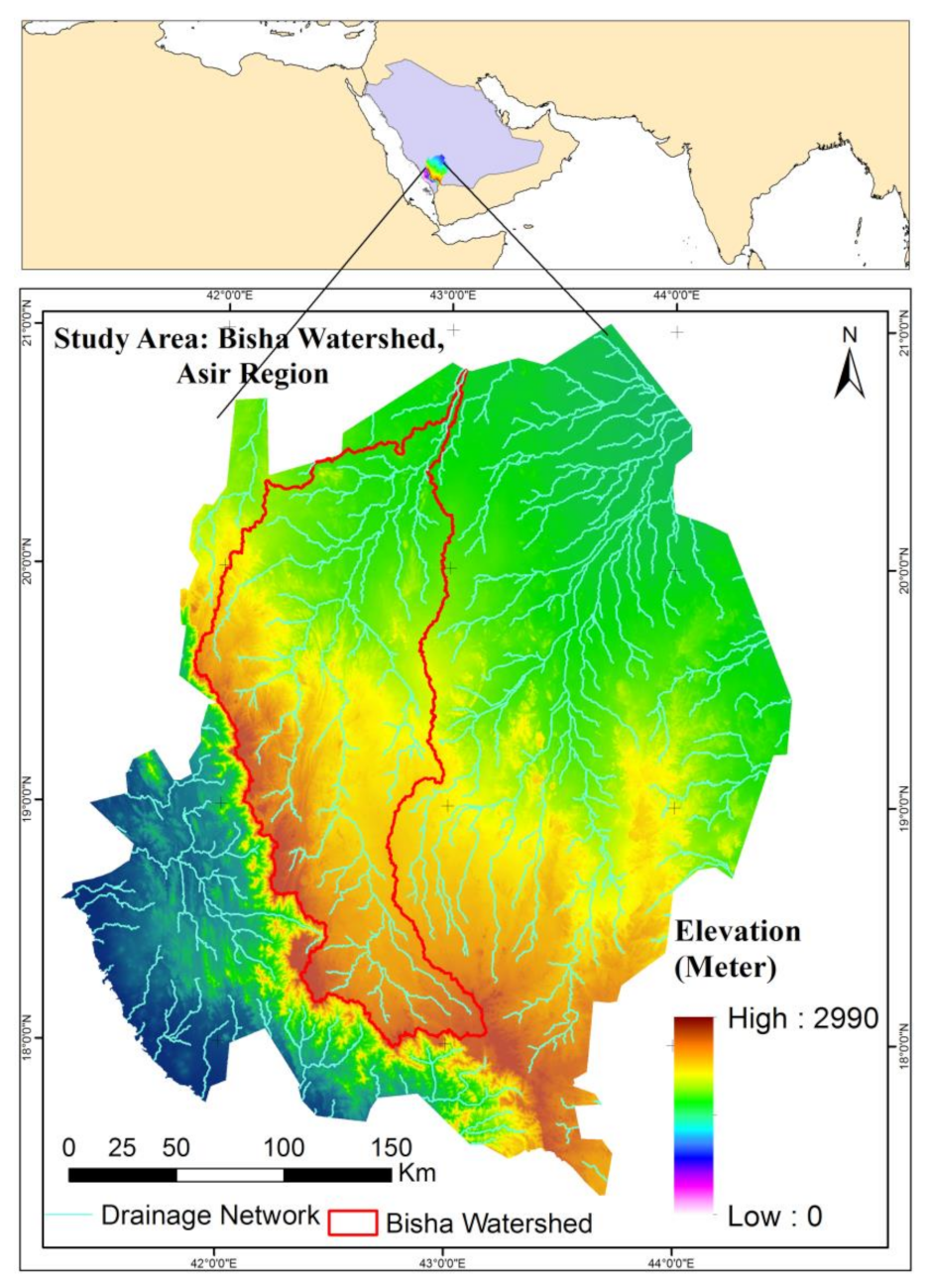
2.1. Study Area

The Bisha watershed, with an area of 21,260 km2, is located in Saudi Arabia’s south-western region and shares a border with Yemen. The Bisha watershed boundaries are found north of the equator, between 17°59′27.588″ N and 20°49′13.958″ N, and east of the Greenwich meridian, between 41°49′50.825″ E and 43°11′20.254″ E (Figure 1). It has a diverse landscape, with highlands, high mountains (between 2000 and 3000 m MSL), plateaus, and Wadiyan. It also includes a large area of the desert to the north and east, stretching all the way to Bisha and Tathlith. The elevation varies between 950 and 2980 m, with a mean of 1655 m. As per the geological settings [79], it is made up of Jurassic–Cretaceous sedimentary rocks (limestone, sandstone, and shale) and Precambrian granite igneous rocks. The region’s climate varies significantly according to geography and season.
The climate varies from semi-arid in the south regions to arid climates in the north. Three meteorological stations operated by Saudi Arabia’s Presidency of Meteorology and Environment serve the study region (PME), namely Abha, Khamis Mushyet, and Bisha. The average temperature in the last 30 years, according to data from three stations, has ranged between 12 °C and 44 °C. The south–west monsoon brings variable rainfall to the highlands of this region [80]. The precipitation results from orographic convection over the scarp in the south-western region of Saudi Arabia, especially during the spring and summer, and are spread out over 2–4 months (March–June), whereas rainfall for the remainder of the period is insignificant [81]. The annual average rainfall is 245 mm. Rainfall exceeding 200 mm per annum is limited to a 20–30 km wide crest zone. Consequently, eastward and northward Wadi flow decreases rapidly downstream, and deposition is greater than erosion near the eastern edge of the plateau.
The rugged landscape of the watershed has aided in biodiversity conservation in the region. The Afromontane, which is part of the watershed, has a corresponding phytogeographic area [82]. The watershed’s highland is surrounded by woodlands and Juniperus procera, which are home to many endemic and rare flora and fauna [83].

2.2. Materials

The groundwater potentiality models for this study were prepared by using fourteen groundwater conditioning parameters. All of these parameters have been extracted from high resolution ALOS PALSAR DEM (spatial resolution: 12.5 m). The DEM has been collected from Earth data of NASA (https://asf.alaska.edu/ (accessed on 7 August 2021).).

2.3. Groundwater Potentiality Inventory

For GWP mapping, several researchers have utilized the positions of springs, wells, and quant for inventory. Well points were taken into account for GWP in this study. The study region’s inventory graph includes 50 well points collected from various resources and detailed site inspection. First, non-groundwater data similar to the groundwater data utilized for GWP modeling must be prepared [84]. The selection was made on the basis of the field survey, with equivalent numbers of non-groundwater data (50 points). The total numbers for groundwater and non-groundwater points are 100. By arbitrary separation, all groundwater and non-groundwater data have been divided into 80% (80 points): a proportion of 20% (20 points) delineates calibrating and test datasets. Model calibration is performed with groundwater and non-groundwater training data, while model validation is performed with groundwater and non-groundwater testing data [22]. Similarly, inventory maps for other areas have been developed.

2.4. Methods for Preparing Groundwater Potentiality Conditioning Factors
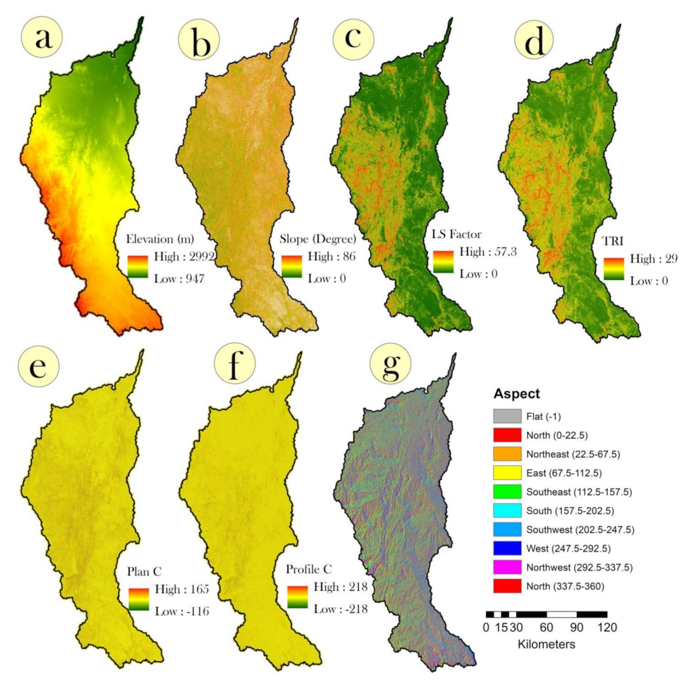
Since it requires multiple variables related to topography and hydrology in geospatial layout, the architecture of the spatial groundwater potentiality model is typically very complex and systematic. As a result, identifying variables that affect groundwater potentiality is critical, and scientifically selected criteria can confirm the accuracy of groundwater potentiality modelling charts. Considering the extensive literature review, data availability and technical setup for GWP modelling in the current study area, the fourteen groundwater potentiality influencing parameters were selected, such as elevation, aspect, TWI, SPI, STI, TRI, TPI, slope, profile curvature, plan curvature, convergence index, topographic feature, slope, flow accumulation, and flow direction. All contributing variables have 12.5 m spatial resolution. In the present study, we used R studio version 4.1.1, ArcGIS version 10.5, QGIS version 3.2, WEKA 3.9, GRASS GIS version 7.4.1, and SAGA GIS version 7.8.2 for machine learning, and we used graphical work, map preparation, and parameters generation from the DEM.

2.4.1. Elevation

The elevation is the most important element in GWP modelling [19]. The potentiality of groundwater is inversely proportional to height. Chen et al. 2020 reported that the probability of groundwater potentiality decreases with elevation and vice versa. As a result, the study area is characterized by relatively flat and low altitude. As a consequence, the presence of groundwater potentiality is normal in the region (Figure 2a).

2.4.2. Slope

The slope, which influences the speed of running water, is also a significant element in influencing the GWP [19,85]. It regulates the amount of water that accumulates in a given region and, thus, acts as an important function in the groundwater recharge operation. The study area is characterized by lower slope and flat areas, which positively influences good groundwater recharge. Therefore, most of the study area has high potential for groundwater (Figure 2b).

2.4.3. LS Factor

The length (L) and steepness (S) of the topography that impacts the quantity of groundwater storage are defined by slope length (LS) (Figure 2c). The following equation is used to compute LS [86]:
L S = ( f a × c e l l s i z e / 22.13 ) 0.4 × ( sin θ / 0.0896 ) 1.3
where fa denotes flow accumulation, and θ denotes the slope in degree.

2.4.4. TRI

The TRI is the most important conditioning variables for GWP modeling [19,20,23]. It was used to measure landscape heterogeneities since it represents the average discrepancy between a central pixel and its neighbouring cells, which affects drainage. As a result, the greater the TRI value, the greater the elevation discrepancy between neighbouring regions since the lower TRI value means higher groundwater content, which is mainly situated at low elevated differences. As a result, low TRI values indicate greater groundwater potential. In this study, the TRI value ranges from 0 to 29 (Figure 2d).

2.4.5. Curvature, Profile, and Plan Curvature

Since curvature influences groundwater allocation, it is used in GWP modelling. It measures the change rate at which a profile line is changed by the angle of inclination of the tangential plane [87]. Ginesta Torcivia et al. [88] and Talukdar et al. [89] reported that the curvature differentiates the convergent and divergent runoff area. Costache and Tien Bui [90] reported that negative value areas are linked to the process of runoff convergence. It influences the flow of water over a surface and mostly governs water retention and groundwater recharge. Therefore, the study area along the river is highly potential for groundwater recharge during the rainy season (Figure 2e,f).
The hydrology of the surface and subsurface is affected by curvature. The greatest slope in specific direction is aligned to the profile curvature. The negative value of profile curvature implies that the water flow in the surface has slowed, while the positive value denotes that the water flow has increased, and zero shows that the surface is flat. Plan curvature, on the other hand, specifies the greatest slope in a perpendicular direction. It depicts how water flowing in the earth’s surface converge and diverge. Negative values reflect the surface’s concave slope, which leads water flow to confluence. Positive values, on the other hand, show that the surface has a convex slope that controls the divergence of water flow in the region.

2.4.6. Aspect

Another factor, aspect, has an effect on the flow paths of groundwater potentiality as well as soil moisture content [91]. It impacts the duration of sunshine, which has an effect on infiltration rates and snowmelt. As a consequence, it has an indirect effect on the GWP (Figure 2g).

2.4.7. Topographic Power Index

TPI is a topographic feature’s slope orientation metric. TPI has been intended to distinguish between the elevation of the central point and the average elevation around the centre point in general. Positive and negative TPI values denote sites that are greater or lesser than the typical surrounding region, respectively, whereas a zero TPI value denotes a flat or continuous slope. The following equation was used to compute the TPI:
T P I = M 0 n 1 M n n
where M 0 denotes the altitude of the middle point, M n denotes the altitude of the grid, and n indicates the total number of pixels in the DEM raster file’s neighbourhood region.

2.4.8. Convergence Index

Convergence index is a smaller-scale measure of the concavity or convexity of the ground. Concavities (e.g., valleys) are represented by negative convergence, whereas convex features (e.g., ridges) are represented by positive convergence. The “system for automated geoscientific analyses SAGA” computed this parameter. Convergence had minimum, maximum, and mean values of −100, 100, and −0.586, respectively (3b).

2.4.9. Topographic Wetness Index

Topographic wetness index is a term that is frequently utilized to illustrate how topography affects the location and length of saturated source areas [92]. It depicts how topography influences runoff generation and the volume of flow that accumulates in a basin. This index depicts the volume of water stored in the area at each pixel scale [93] and is measured using Equation (3).
T W I = I n ( A s ) tan β
As is the entire upslope catchment area flowing downward from a slope angle of β. In general, high TWI values and GWP have a robust relationship [94]. The study area has TWI value ranges from 4.1 to 19 (See Figure 3c).

Stream Power Index

Another variable that influences the groundwater potentiality is SPI, which measures the stream’s erosive strength [95]. Equation (4) is used to calculate the SPI.
  S P I = A s tan β
A s indicates the catchment area, while β denotes the slope. The SPI in the study area ranges from 0 to >12.6 (Figure 3d).

2.4.10. Flow Direction

After the depressions have been corrected, each cell in the grid is allocated to flow across the DEM surface, which is continuous [96]. The flow direction of a cell may be described as the direction in which water and sediment would flow out of that cell, regardless of the many techniques employed to determine flow direction in the grid. The D-8 technique assigns the flow direction for each cell in a grid to one of the eight neighboring or diagonal neighbouring cells in the direction with the steepest downhill slope. As a result, considering the flow direction and resolution of any cell, the distance travelled by a flow may be calculated by using the basic Euclidean distance between cell centres, which is dependent on cell size (1 unit cell size for N–S and E–W; 1.414 for diagonals) [96]. As a result, the total flow length at each particular cell in the watershed may be computed. The flow direction was determined using the SRTM digital elevation model, and it is currently used as a crucial input component for determining the flow length.

2.4.11. Flow Accumulation

The upslope area flowed from a point in topographic orientation is referred to as flow accumulation or upslope contributing area. The flow accumulation computed from the DEM could be used as a proxy for ridgelines, residual soil sites, colluvium concentration, moisture availability, and drainage flow lines [97]. Flow accumulation influences how slope materials and rainwater are spread, as well as where water and slope material flows tend to accumulate. The former is defined as divergent slopes, while the latter is regarded as convergent slopes, and both are potential locations for colluvium and saturation, as well as recharge and seepage zones.

2.4.12. Topographic Features

Topographic influences are critical for GWP modelling because they affect the hydrological characteristics of the research region both directly and indirectly [98,99]. At first, a Digital Elevation Model (DEM) was generated in ArcGIS 10.5 from the ALOS PALSAR DEM for the study area. From the DEM, we extracted topographic features in the SAGA GIS QGIS software.

2.5. Method for Groundwater Potentiality Conditioning Variables Using Multicollinearity Test

In flood susceptibility mapping, the multicollinearity test is a crucial step. Multicollinearity refers to the presence of a linear relationship between several or all of a regression model’s independent parameters [84]. A division-by-zero in regression calculation might be caused by the existence of a linear connection between variables. This issue can result in erroneous computations, and dividing by a little number can cause the findings to be skewed.
Multicollinearity is a method that uses strongly interrelated independent variables in a logistic regression model. It indicates that one variable may be predicted with a high degree of accuracy linearly from the others. Multicollinearity has no effect on the model’s predictability or dependability. It only has an impact on individual predictor estimations [100].
Variance inflation factors (VIFs), pairwise scatter plots, and eigenvalues in a correlation matrix are some of the approaches that may be used to discover multicollinearities. For each flood conditioning parameter, VIF is utilised to detect multicollinearity in this study. The VIF is a statistic that evaluates the strictness of multicollinearity by using a least squares regression. In the present study, VIFs have been used for analyzing multicolinearity.

2.6. Proposing Fuzzy Logic-Information Gain Ratio Weighting Based Hybrid Models for Groundwater Potentiality Mapping

In order to improve the precision of groundwater potentiality models, hybrid FL models have been generated by integrating fuzzy operators with information gain ratio. This was accomplished by a series of steps. The thirteen topographic and hydrologic parameters were used to construct groundwater potential models by using fuzzy logic model and information gain ratio. The details of fuzzy logic and information gain ratio-based hybrid models are as follows.
It is critical to evaluate the importance of the groundwater potentiality influencing parameter before practicing and validating the model [101]. Based on mathematical properties and interactions with groundwater, the value of each collected parameter has been quantified. The information gain ratio, i.e., InGR technique [99], was used to define the influential parameters for groundwater potentiality prediction. InGR significance is assigned to each determining factor to quantify its relevance. The higher the InGR rating, the more important the influence factor. The InGR model was selected for use in this analysis due to its consistency and efficacy, and it is measured using Equation (5):
  G a i n _ r a t i o ( x , Z ) = E n t r o p y ( Z ) 1 n i = 1 n Z i Z E n t r o p y ( Z i ) i = 1 n Z i Z log Z i Z
where the feature, x, belongs to the training point Z with Z i 1 = 1 ,   2 ,   3 , . n subsets,.
Using the information gain ratio and ground truth data, the weights for all parameters have been derived. Then, the weights were assigned to the parameters in the raster calculator of the ArcGIS 10.5 software.
Zadeh was the first to present fuzzy set theory [102]. It allows for the mathematical understanding of non-discrete natural phenomena [103]. The membership value of elements ( x ) has various degrees of support and confidence ( f ( x ) ) in the range (0, 1), according to this theory [104]. The following formula may be used to describe a fuzzy set:
A = x , f a ( x ) , x R
where A denotes a fuzzy set, x represents universal element set R , and f ( x ) denote the fuzzy membership function.
The membership value of a crisp set range (0, 1) is either 1 or 0, but a fuzzy set inherits continuous membership in the range (0, 1). Groundwater potential mapping necessitates the establishment of a fuzzy membership function of causal components. A membership function can be provided quantitatively by using mathematical equations depending on the data type (ordered or categorical) and its relationship with the dependent variables. In the present research, thirteen parameters have different data types and nature; therefore, different types of membership function have been used. The MS-Small has been used to create fuzzy crisp layers, such as elevation, slope, aspect, topographic features, flow direction, LS factor, and TRI. It determines membership by relying on the input data’s mean and standard deviation, with small values indicating high membership. On the other hand, MS-Large function was used to transform the layers into fuzzy crisp layers, such as profile curvature, plan curvature, flow accumulation, flow direction, SPI, TPI, and TRI. It determines membership by relying on mean and standard deviation of the input data, with large values indicating high membership. Thus, we transformed weighted data into simplified, normalized, and unidirectional fuzzy crisp layers
The fuzzy operation is the next stage in the fuzzy logic method. Important fuzzy operators include fuzzy OR, fuzzy AND, fuzzy algebraic sum, fuzzy algebraic product, and fuzzy gamma operator [105]. Only one of the contributing fuzzy sets has an influence on the resulting value in fuzzy OR and fuzzy AND. The fuzzy algebraic sum and fuzzy algebraic product operators, respectively, render the output set greater or equal to the maximum value and smaller or equal to the minimum value across all fuzzy sets [106]. The fuzzy gamma ( γ ) operator produces values that fall between the fuzzy algebraic product and fuzzy algebraic sum. The γ value ranges from 0 (no compensation) to 1 (full compensation). The degree of compensation between two extreme confidence levels is used to determine the optimal γ value.
In GPM investigations, the use of an appropriate fuzzy operator for data integration is essential for obtaining the best results. The type of geographic data to be integrated determines the fuzzy operator to use. All of the 13 criteria considered in this analysis included equal amounts of data. Data integration can be performed by using a mix of fuzzy operators or multiple distinct fuzzy operators depending on the nature of the spatial data. We employed all operators to integrate the fuzzy crisp layers in this investigation. The following formula was used to integrate fuzzy crisp layers:
f A N D = M I N f E l e , f S l o p e , f A s p e c t , f T W I , f T R I , f S P I , ..
f O R = M A X f E l e , f S l o p e , f A s p e c t , f T W I , f T R I , f S P I , ..
F u z z y   A l g e b r a i c   P r o d u c t = i = 1 n R i
F u z z y   A l g e b r a i c   S u m = 1 i = 1 n ( 1 R i )
f γ = ( F u z z y   A l g e b r a i c   S u m ) γ × ( F u z z y   A l g e b r a i c   P r o d u c t ) 1 γ )
where f E l e , f S l o p e , f A s p e c t , f T W I , f T R I , and f S P I are fuzzy crisp layers of elevation, slope, aspect, topographic wetness index, topographic ruggedness index, and stream power index, respectively. Moreover, R i represents the fuzzy membership function of the i th map, i = 1 , 2 , , n . The GPMs were created by applying the fuzzy gamma operator on the results of Equations (6), (7), and (10). Six distinct GPMs were prepared by using the following six values: AND, OR, GAMMA0.8, GAMMA 0.85, and GAMMA 0.9. GPM maps are raster data that are ordered and continuous, with each grid/cell quantitatively depicting the degree of ground water potentiality. GPM is measured using fuzzy operators in a variety of ways (0, 1). By using Jenk’s Natural Break (ESRI 2012) categorization, these GPM maps were divided into five categories: very low, low, moderate, high, and very high potentiality. GPM maps were created accordingly.

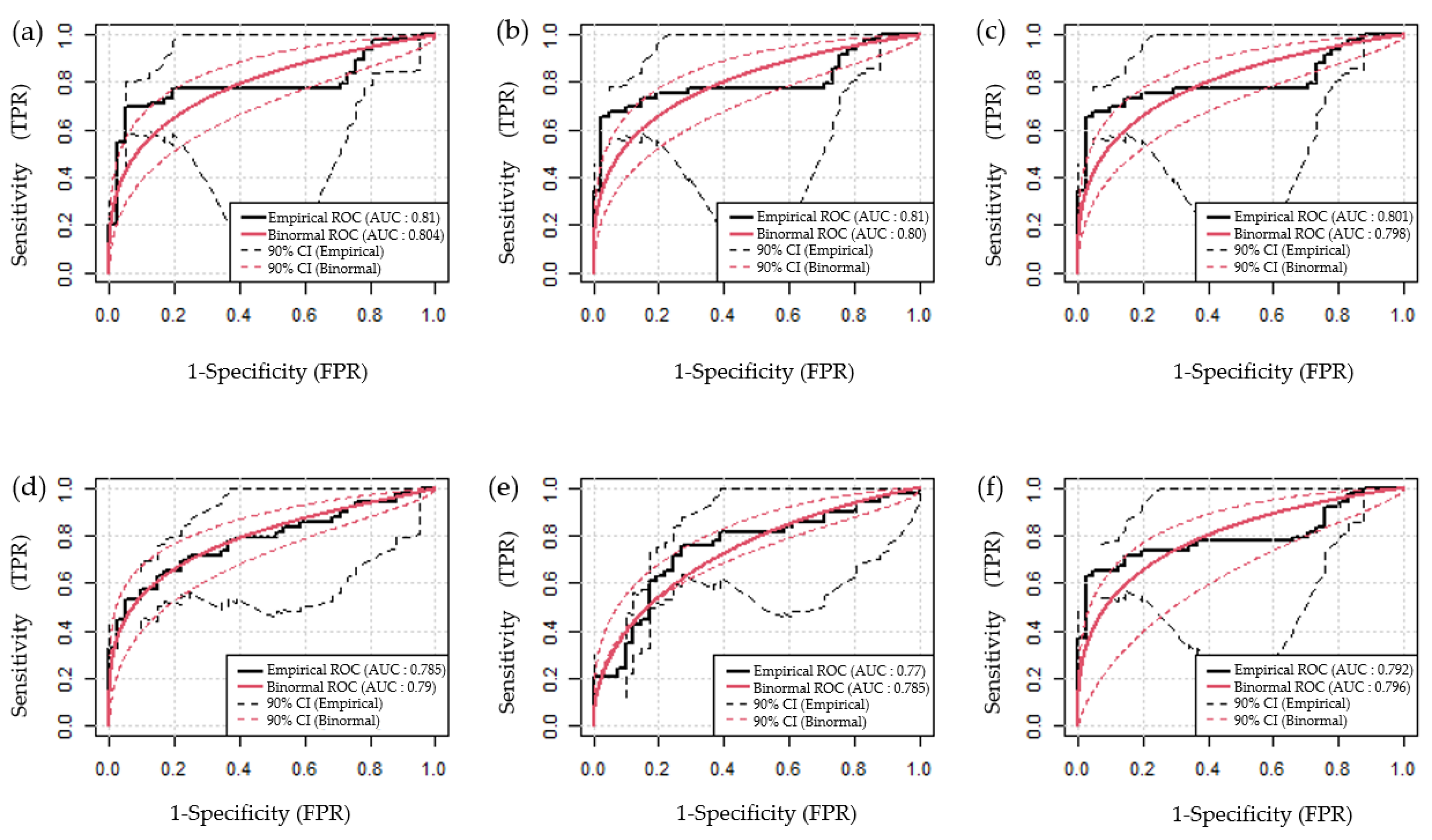
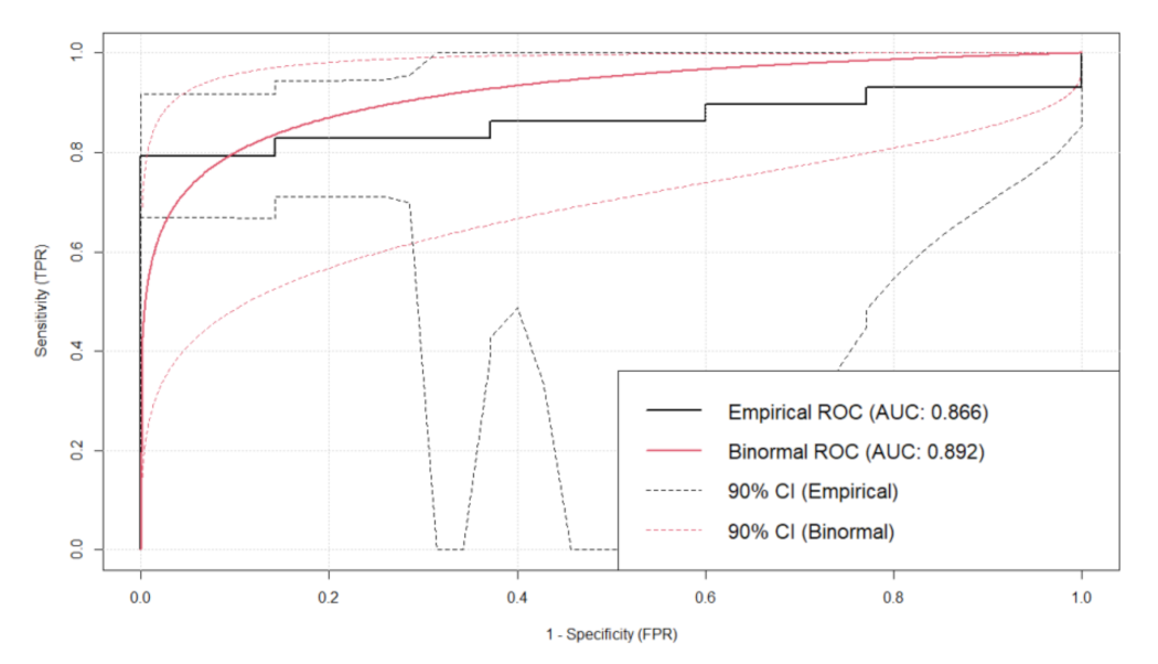
2.7. Validation of the Models

The ROC curve is a graphical representation of the sensitivity (TPR) on the y-axis and the specificity (FPR) on the x-axis for different cut-off points of test data. For convenience, it is usually shown as a square box, with both axes ranging from 0 to 1. The AUC is a useful metric of sensitivity and specificity that may be used to examine a diagnostic test’s intrinsic validity. AUC = 1 indicates that the diagnostic test is completely accurate in distinguishing between groundwater and non-groundwater [24]. This means that sensitivity and specificity are equal, and both false positive and false negative errors are zero. In actuality, this is quite unlikely to occur. The closer the AUC is to one, the better the test performance. The diagonal from (0, 0) to (1, 1) divides the square into two equal pieces, each with an area of 0.5. When the ROC is at this line, the test has a 50/50 probability of accurately distinguishing between groundwater and non-groundwater. The minimal AUC value should be 0.5 rather than 0 since AUC = 0 indicates that the test wrongly categorised all subjects with groundwater as negative and all non-groundwater subjects as positive. When the test findings are reversed, area = 0 becomes area = 1; therefore, a completely incorrect test can be converted into a perfectly accurate one.
The area under the ROC curve was calculated by using both non-parametric and parametric techniques. The user must make a decision. The parametric technique, on the other hand, has been frequently used to validate prediction models. Both parametric and non-parametric techniques were utilised in this research.

2.7.1. Non-Parametric

This does not need any test value distribution pattern, and the resulting area under the ROC curve is referred to as empirical. The first technique employs the trapezoidal rule. It simply joins the points at each interval of the recorded values of the continuous test and creates a straight line connecting the x-axis to determine the area. This creates a number of trapezoids, each of which can be simply computed and totaled.

2.7.2. Parametric

When the statistical distribution of diagnostic test results in positive and negative subjects is known, these are employed. For this, a binormal distribution is often employed. When test values in both positive and negative subjects have a normal distribution, this is relevant. The necessary parameters may be simply calculated by using the means and variances of test scores in positive and negative subjects if the data are really binormal or if a transformation such as log, square, or Box-Cox renders the data binormal. An AUC of >70% would be considered satisfactory model performance in this situation [107].

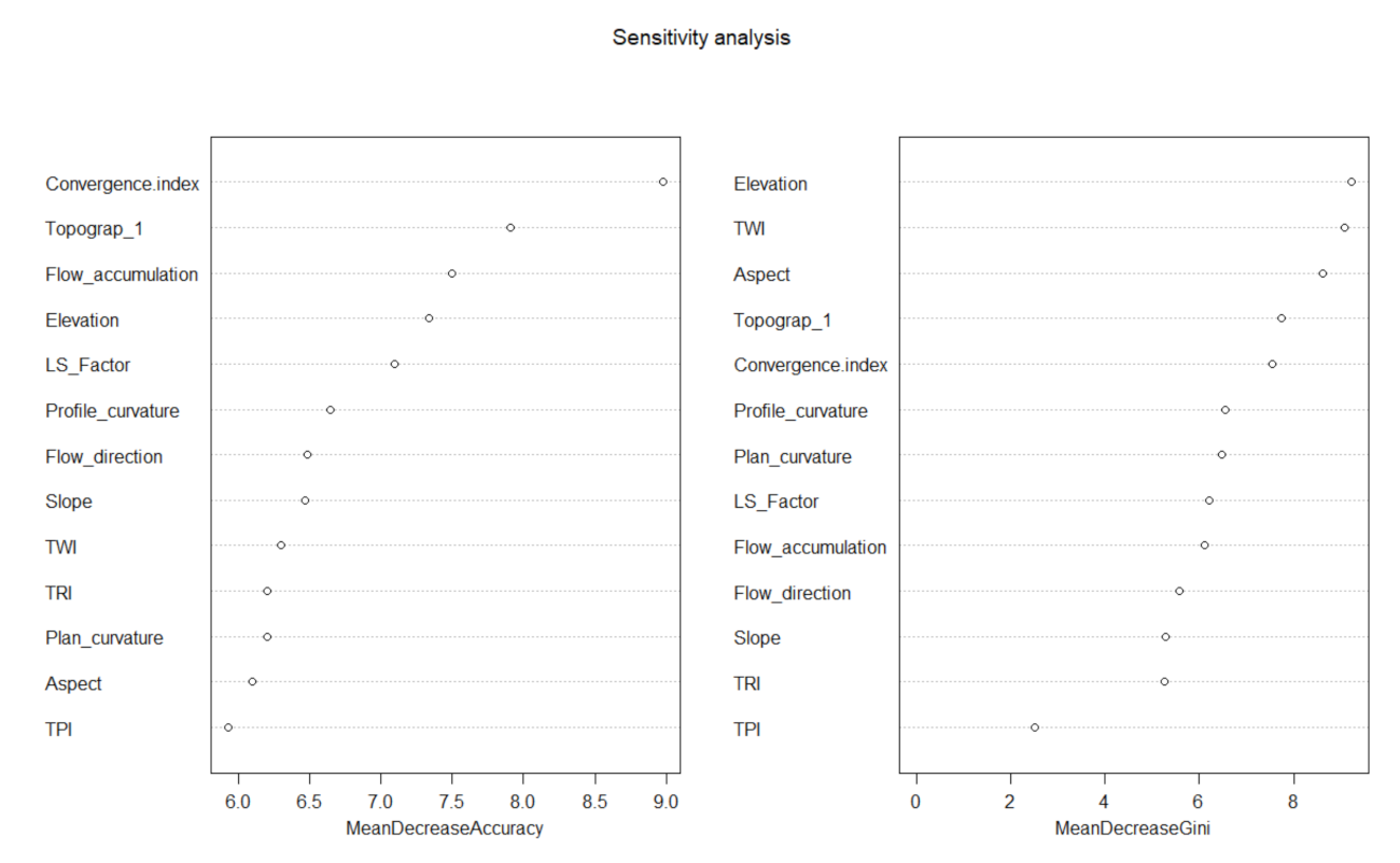
2.8. Sensitivity Analysis

Random forest offers two distinct important metrics for ordering variables and variable choice, mean decrease accuracy (MDA), and mean decrease Gini (MDG). When the values of a variable become randomly permuted relative to the original data, MDA evaluates the significance of the variable by evaluating the change in prediction accuracy [100]. MDG is the total of all Gini impurity reductions caused by a particular variable (when that variable is used to generate a split in the random forest), normalised by the number of trees.

2.9. Proposing LR-Based Novel Hybrid Model for Groundwater Potentiality Mapping

In order to improve the precision of groundwater potentiality models, LR was paired with previously applied and current hybrid models. This was accomplished by a series of steps. In the first round, information gain ratio-based weightage technique and six operators of fuzzy logic were integrated in order to construct groundwater potential models. The following procedure was used to integrate statistical models, such as LR with the hybrid models for obtaining higher accuracy in groundwater potential models. For incorporating the LR models, we used six newly developed models as parameters. Testing datasets (20% of the total datasets) were used to collect data from the six hybrid models, and they were held exclusively for validation purposes. The aim of using validation datasets and ensemble models was to determine how well the newly generated hybrid models predicted groundwater potentiality. Another significant advantage of using validation datasets for second-step modelling is that they can be used for any modelling purpose. As a result, it can provide outstanding ground truth proof for obtaining exceedingly detailed information about the outputs of newly developed hybrid models. The validation data was used for combining LR and hybrid groundwater potentiality models using the collected data. In the next stage, six hybrid models have been weighted by using the weights of six hybrid groundwater potentiality models derived from the LR models. Then, weighted parameters were integrated in a raster calculator; thus, an LR-based novel hybrid model has been constructed. In the last stage, the hybrid model has been validated using ROC curve in order to observe how accurately the hybrid model predicts the groundwater potential zones. Some details of the LR are as follows

Logistic Regression

The probability of an event is weighed against a number of potentially predictive variables in LR (LR), which is one of the most widely used statistical techniques. In the case of groundwater potentiality prediction, the expected occurrence has been defined as groundwater or non-groundwater, and the purpose of LR is to determine the best suitable algorithm to evaluate the relationship between a set of conditioning variables and the appearance or absence of groundwater [108]. In addition, as LR uses its convergence criterion to maximise the likelihood function [109], its predictive success in classification problems is considered to be very exceptional [110].

3. Results

3.1. Multicolinearity Analysis

VIF and Tolerances (TOL) were utilised to determine multicollinearity between independent variables in this study. A multicollinearity problem is indicated by a VIF score of >10 and a tolerance value of 0.2. The VIF and tolerance values of all factors are less than 10 and more than 0.2, respectively, according to the results of the multicollinearity test. As a result, there is no concern with multicollinearity among independent variables. As a result, in the current study, all nine flood conditioning variables were taken into account while creating the FS map. The following are the results of Multicollinearity analysis for the present study: elevation (VIF: 1.327, TOL: 0.753); aspect (VIF: 1.382, TOL: 0.724); slope (VIF: 1.242, TOL: 0.805); LS factor (VIF: 1.48, TOL: 0.7); plan curvature (VIF: 2.599, TOL: 0.385); plan curvature (VIF: 1.952, TOL: 0.512); TPI (VIF: 1.847, TOL: 0.541); TRI (VIF: 1.65, TOL: 0.67), TWI (VIF: 1.911, TOL: 0.523); convergence index (VIF: 1.498, TOL: 0.667); topographic feature (VIF: 4.720, TOL: 0.212); flow accumulation (VIF: 1.472, TOL: 0.679); flow direction (VIF: 1.198, TOL: 0.834); and SPI (VIF: 5.379, TOL: 0.186).

3.2. Proposing Feature Selection Based Hybrid GW Potentiality Models

In the present study, in order to propose feature selection approach integrated fuzzy logic models, a variety of steps have been followed. The initial collections of variables have varying levels of predictability. Including all factors in the study, on the other hand, may diminish the predictive power of the generated models. As a result, the predictive capacity of the elements used in the study should be assessed, and components that have a negative impact on the accuracy of the created models should be eliminated. For these purposes, data from 14 CFs were retrieved on the basis of the training datasets. The weights for all parameters were then calculated by using the information gain ratio (IG) method. This procedure will aid in the development of more accurate prediction models. Based on the IG findings, it could be stated that no parameters have negative prediction power; hence, no parameters have been removed from the modelling of GWP. Since the IG value indicates predictive power, we used these values as weights for all factors in our analysis. The parameters were then allocated weights. As a result, the normal parameters have been converted into weighted parameters. The following are the obtained IG values for all CFs: elevation (IG: 0.482); topographic feature (IG: 0.274); flow accumulation (IG: 0.228); flow direction (IG: 0.168); slope (IG: 0.146), TWI (IG: 0.142); TRI (IG: 0.138); aspect (IG: 0.103); LS factor (IG: 0.103); convergence index (IG: 0.1002), SPI (IG: 0.1001); plan curvature (IG: 0.094); profile curvature (IG: 0.091); and TPI (IG: 0.011).
Following the generation of the weighted parameters, the parameters were converted into fuzzy crisp layers using the fuzzy membership function. The membership functions that were picked for different variables are specified in the Materials and Methods Section. The fuzzy membership functions, on the other hand, were chosen based on the data types and their contribution to groundwater potentiality modelling. As a result, the fuzzy membership function also served as a weightage mechanism.
Following the transformation of the fuzzy crisp layer, the fuzzy operators AND, OR, GAMMA0.75, GAMMA0.8, GAMMA0.85, and GAMMA0.9 were used to integrate the fuzzy crisp layers. As a result, hybrid fuzzy models for groundwater potentiality were created. Following that, the natural break algorithm was used for the resulting fuzzy models, which range from 0 to 1 in value (with 1 indicating high potentiality and 0 indicating low potentiality), for classification. There are five groundwater potentiality classifications, including very high, high, moderate, low, and very low groundwater potentiality zones.
Figure 4 represents the groundwater potentiality models as constructed using advance hybrid algorithms, such as AND, OR, GAMMA0.75, GAMMA0.8, GAMMA0.85, and GAMMA0.9. As shown in Figure 4, the potential zones of groundwater were divided into five categories: very high, high, moderate, low, and very low. The potential groundwater zone runs in a northwest–southeast direction, parallel to the drainage direction of the catchment. The south and southeast are dominated by zones with high groundwater potential, whereas the north and northwest are dominated by areas with low groundwater potential zones.
Around 1850–2149 km2 and 3644–4585 km2 areas to the total basin area are found to have ‘very high’ and ‘high’ potentiality for groundwater, respectively, in the case of the RF model (Table 1). In general, all of the models defined the river catchment area as having a lot of potential for underground water harvesting. However, since there are variations in the size of the region, it is critical to explain the best representative model.

3.3. Validation of the Models

The AUC of empirical and binormal ROC was used to validate the generated GPMs utilising the collected GPS points. The resulting AUCs under the respective ROC (empirical and binormal) are 0.81 and 0.805 for AND; 0.81 and 0.80 for OR; 0.801 and 0.798 for GAMMA0.75; 0.785 and 0.79 for GAMMA0.8; 0.77 and 0.785 for GAMMA0.85; and 0.792 and 0.796 for GAMMA0.9 (see Figure 5a–f). Based on both ROC curves, AND appeared as the best model, followed by OR, GAMMA0.75, GAMMA0.9, GAMMA0.8, and GAMMA0.85. However, as per the binormal ROC curve, which has widely been applied for natural hazards, AND appeared as best model (AUCb: 0.805), followed by OR (AUCb: 0.8), GAMMA0.75 (AUCb: 0.798), GAMMA0.9 (AUCb: 0.796), GAMMA0.8 (AUCb: 0.79), and GAMMA0.85 (AUCb: 0.785). Although all models achieved AUC values near 0.8, they can be considered as satisfactory results. However, many researchers obtained AUC values of more than 0.4. Due to absence of other climatic, land use, hydrologic, and geological data, the generated hybrid models achieved little bit lower accuracy. In addition, the application advanced machine learning algorithms can also produce highly accurate models. However, in order to improve these models further, the LR has been recommended for utilization. As a result, the absence of other parameters can be overlooked.

3.4. Sensitivity Analysis

The development of advanced hybrid algorithms for mapping groundwater potential zones can only show the probable region enclosing the future occurrence of a significant and a quantity of groundwater supplies that can be commercially used based on the complex mathematical relationship between historical groundwater trends and their triggering variables. Neither of these models, however, mentions the role of any variables in the declining trend of groundwater potential in an area. The question arises as to how management plans can be planned and implemented if the effect of such factors on the occurrence of landslides cannot be determined.
How will management plans be developed, and how will management plans be implemented if the effect of such conditions on groundwater potentiality cannot be determined? Identifying variables related to groundwater potential zones may aid in reducing the frequency of groundwater decline in a given region. Therefore, it is crucial to figure out which variables have the most influence. In order to estimate the relevance of each conditioning variable in the RF modelling process, the mean decrease in Gini (MDG) and mean decrease in accuracy (MDA) have been employed [111]. The findings (based on MDG and MDA) show that all factors were included in the GWP modelling, but the most important ones were convergence index, topographic features, flow accumulation, elevation, LS factors, flow direction, profile curvature, and slope (Figure 6). TPI, aspect, and TRI were the least important determinants in establishing the relative significance of the 14 variables included in the hybrid models (Figure 6).

3.5. Development of LR-Based Hybrid Model and Its Validation

This study utilizes six hybrid algorithms for mapping groundwater potential zones. Furthermore, a sensitivity model based on RF was used to describe the sensitive parameters of these potential groundwater models. All of these models performed very well for predicting potential groundwater zones, according to the results of the ROC’s AUC values, using AND, OR, GAMMA0.75, GAMMA0.8, GAMMA0.85, and GAMMA0.9 models. Nonetheless, this study aimed to improve the precision and reliability of groundwater potential mapping by integrating statistical models such as LR models with previously created potential groundwater zone models. We used all the nine groundwater potential models that had already been developed by using the machine learning algorithms. After integrating six groundwater potential maps with mathematical models, the error for over and underestimation of all models can be eliminated. The LR model’s characteristics are as follows: The Chi-square significance was greater than 0.05 in the Hosmer–Lemeshow test, indicating that the equation’s fitting goodness could be calculated. The independent variables could explain the dependent factor according to the Cox and Snell (R2) and Nagelkerke (R2) values (Cox and Snell R2: 0.171; Nagelkerke R2: 0.233). The following is how the LR was calculated (Equation (12)).
1.62 + (OR × 0.23) + (GAMMA0.8 × 0.053) + (GAMMA0.85 × 0.004) + (GAMMA0.9 × 0.061) + (GAMMA0.75 × 0.0012) + (AND × 0.31)
The performance of the LR-based novel hybrid ensemble models is shown in Figure 7. The groundwater output was divided into five subclasses using the natural break algorithm (from very high to very low). The very high groundwater potential zone was estimated by the novel hybrid model to be 1635.92 km2, followed by high (3235.88 km2), moderate (5233.84 km2), low (6001.85 km2), and very low (5165.05 km2).
Then, by using the ROC curve, we validated the novel hybrid groundwater potential model by using the testing dataset. The new model’s AUC values (AUCe: 0.866, AUCb: 0.892) indicate that it is extremely accurate and informative in estimating potential groundwater zones (Figure 8). It also outperformed the six hybrid models, implying that combining an advanced hybrid model with a statistical model would improve model accuracy even more.

4. Discussion

In areas with limited surface water, particularly in dry and semi-arid climates, groundwater supplies are critical. When these regions’ industrial and agricultural water needs are high, aquifers can be depleted at rates that surpass recharge rates, placing them in danger of irreversible harm. As a result, precise estimates of the spatial dimensions of groundwater in a watershed are critical. Assessments such as these can help with water management planning and usage strategies. By understanding the geomorphological and hydrological conditioning variables connected with subsurface storage, groundwater mapping may be enhanced and made more cost-effective. In order map groundwater potential, several approaches have been devised, each with its own set of benefits and drawbacks.
To map groundwater potential, this study created a unique state-of-the-art method that combined statistical, machine-learning, and feature selection approaches with RS and GIS tools. To assist scientific judgments for issues with a variety of management criteria, feature selection techniques, statistical models, and machine-learning algorithms (such as information gain ratio, fuzzy logic, and LR, respectively) have been utilised. The very high groundwater potential zone, according to the results of six advanced hybrid models and one novel hybrid model, encompasses an area of 1635–2149 km2. The groundwater potential models were evaluated by using an empirical and binormal ROC curve. AND (AUCe = 0.81; AUCb: 0.804) was the best representation model for groundwater potentiality modelling based on both ROC curves, followed by OR, GAMMA0.75, GAMMA0.9, GAMMA0.8, and GAMMA0.85. On the other hand, the novel hybrid model achieved higher accuracy (AUCe: 0.866; AUCb: 0.892). This model outperformed the six hybrid models. The integration of all hybrid models through the LR model has eliminated the mis-classified area. Therefore, the novel hybrid model performed better and can be used for other areas, although higher accuracy can be achieved if all kind parameters have been integrated. According to our findings, GW managers in the study area region should concentrate on expanding GW exploitation and agricultural operations in the area close to rivers. Since they receive more natural recharge, these locations have a larger GW potential.
Convergence index, topographic feature, flow accumulation, altitude, LS, and slope degree all contributed significantly to the GW potential investigation. Convergence affects the flow speed on the slopes, which in turn affects erosion and sedimentation, which in turn affects the infiltration rate and GW potential indirectly. TWI is a hydrological conditioning variable that relates to the likelihood of water accumulation in different areas of the basin and, as a result, influences the basin’s GW potential. The fourth most critical factor in modelling was altitude. Higher elevations have steeper slopes and increased flow velocity, resulting in higher drainage density, whereas lower altitudes have the opposite scenario. Regarding the large topographical variance in the studied region (947 to 2992 m), this aspect contributed significantly to the GW potential in our study. SPI, LS, and slope degree, among other significant conditioning variables (CF), have an influence on flow speed and infiltration rate and are, thus, listed as top contributors in this study. In estimating GW potential, Rahmati et al. [112] demonstrated the relevance of the two categorical conditioning factors of land use and lithology. Furthermore, they stated that TWI was the least important CF, which contradicts the findings of this study. According to Mousavi et al. [113], the top contributing CFs are TWI, height, distance from rivers, river density, distance from faults, and fault density. Yousefi et al. [114] presented a work that stressed the relevance of TWI and altitude variables in groundwater potential mapping, which is consistent with the findings of our study. Despite the fact that the two critical CFs connected to the fault layer were not included in this investigation, the algorithms produced high-accuracy GPMs. This demonstrates that substituting simpler calculation-process factors such as DEM-derived CFs for the key component in GW modelling may nevertheless achieve excellent accuracy.
LR-based novel hybrid model outperformed fuzzy-based hybrid models when it came to groundwater potentiality models. Based on these findings, the paper recommends utilising hybrid models and ensemble models for multi-parametric spatial prediction. To the authors’ knowledge, although there has been no previous study that used these models in this study area, it should be noted that the LR-based hybrid model has demonstrated good performance in other environmental fields such as livelihood risk prediction [115,116], groundwater salinity [117], stream-flow prediction [118], piping erosion [119], and flash-flood hazard assessment [120,121]. However, it can be noted that state-of-the-art machine learning models outperform older approaches in most cases [121]. Ensemble models, in particular, frequently outperformed single models [122]. For groundwater potential mapping, Mosavi et al. [123] assessed four ensemble models, i.e., Boosted generalized additive model (GamBoost), adaptive Boosting classification trees (AdaBoost), Bagged classification and regression trees (Bagged CART), and random forest (RF), and found that the Bagging models (i.e., RF and Bagged CART) had a higher performance than the Boosting models (i.e., AdaBoost and GamBoost). This indicates that ensemble models outperformed other traditional ensemble models. Therefore, based on the previous literature, it can be stated that the generated hybrid models could be reliable and used for management strategies. This study also suggests that a few more hydrogeological and meteorological factors should be included in the models in order to improve the accuracy of the results. The study area is known for its water scarcity due to damming across the river and other human issues. Such information might be useful in developing long-term water harvesting and agricultural plans. Water bodies have been recognised as a good conditioning factor for groundwater potentiality; therefore, rapid reclamation of water sources should be avoided at all costs. According to this research, land cover and canopy density are also significant conditioning factors. Forest loss and devastation, on the other hand, are irrefutable realities. As a result, maintaining forest cover will help groundwater recharge. A scientific study of groundwater at distinct prospective zones is required in order to make a more accurate suggestion on the amount of water that may be collected from each potential zone.
The results obtained are exclusive to this study, and they may differ in other investigations due to the fact that the input data for modelling vary from one location to another. As a result, possible models must be considered, with the best predictive capability-based model being chosen to aid in the identification of high groundwater potential regions in order to alleviate drought. Moreover, the novel technique can be useful in areas where there is a shortage of precise and high-resolution data, such as land use, lithology, soil, hydrogeology, and fault-related variables such as fault density and distance from faults.

5. Conclusions

The goal of this research study was to introduce a novel approach for determining GW potential by using a limited amount of high-resolution input data. For GPM, the suggested system used a weighted six fuzzy operator’s model with logistic regression to implement feature selection. The novel hybrid model outperformed the six fuzzy-based hybrid models and provided trustworthy GPMs according to the results. The novel hybrid model’s higher accuracy might be due to its capacity to provide more broad outputs and deal with overfitting. All of the models projected the same regions with extremely high GW potential. The reliability of the technique is demonstrated by the GPMs’ consistency. The major goal of this work was to establish precise GPMs in the study region using solely DEM-derived variables. The relevance of the novel technique was demonstrated in the absence of other major CFs owing to the algorithms’ high AUC values. The results indicated that convergence, TWI, altitude, SPI, and LS all have a significant role in the algorithms’ performance. As a result, in the absence of other key CFs including land use, lithology, soil, and fault-related CFs, the novel hybrid algorithms successfully extracted connections between DEM-derived variables and GW potential. Since we only need a few numbers of datasets covering DEM and groundwater locations, the suggested methodology may be utilised for large-scale GW potential mapping at the nation and continent levels. It should be noted that the established technique is suggested for assessing GW potential through topographically driven groundwater locations. This technique may provide water sector managers and GW experts with the knowledge they need to establish appropriate water resource planning. Scholars may focus future studies on the DEM’s spatial resolution and other DEM-derived variables in order to enhance the technique and, as a result, the modelling outcomes.
The absence of information on groundwater productivity features such as as transmissivity and specific capacity further hampered our investigation. In future research, when these data are available, it is suggested that the relationship between these parameters be explored. Despite the drawbacks, the groundwater potential maps projected in this work can assist water resource managers and policymakers in the disciplines of watershed and aquifer management in preserving the best possible use of this vital freshwater resource.
The superior models developed in this work might be useful with respect to water resource managers in identifying susceptible areas and developing and enforcing appropriate groundwater management regulations. Hybrid machine learning approaches and deep learning are strongly recommended for future study in order to discover an ideal model with a greater level of adaptivity, accuracy, and generalisation ability.

Author Contributions

Conceptualization, J.M., M.K.A. and A.R.M.I.; data curation, J.M., S.T. and M.A. (Majed Alsubih); formal analysis, J.M., S.T. and M.A. (Mohd. Ahmed); funding acquisition, J.M.; investigation, N.B.K.; methodology, J.M., S.T. and N.B.K.; project administration, J.M., N.B.K. and M.K.A.; resources, S.T., N.B.K., M.A. (Mohd. Ahmed), M.A. (Majed Alsubih), M.K.A. and A.R.M.I.; software, S.T.; supervision, M.A. (Majed Alsubih); validation, J.M. and S.T.; visualization, N.B.K., M.A. (Mohd. Ahmed) and M.A. (Majed Alsubih); writing—original draft, J.M., S.T. and M.A. (Mohd. Ahmed); writing—review and editing, N.B.K. and A.R.M.I. All authors have read and agreed to the published version of the manuscript.

Funding

Funding for this research was given under award numbers IFP-KKU-2020/13 by the Deanship of Scientific Research; King Khalid University, Ministry of Education, Kingdom of Saudi Arabia.

Institutional Review Board Statement

Not applicable.

Informed Consent Statement

Not applicable.

Data Availability Statement

The data presented in this study are available on request from the corresponding author.

Acknowledgments

The authors extend their appreciation to the Deanship of Scientific Research, King Khalid University, Ministry of Education, in Saudi Arabia for funding this research work through the project number IFP-KKU-2020/13.

Conflicts of Interest

The authors declare no conflict of interest.

List of Acronyms

GPM:Groundwater potential model
LR:Logistic regression
DEM:Digital elevation model
ROC:Receiver operating characteristic
ROCe:Empirical receiver operating characteristic
ROCb:Binormal receiver operating characteristic
CGWB:Central Groundwater Board
BCM:Billion cubic metres
GIS:Geographic information system
NDVI:Normalized Difference Vegetation Index
TWI:Topographic wetness index
TRI:Terrain Ruggedness Index
SPI:Stream power index
EBF:Evidential belief function
SI:Statistical index
WoE:Weight of evidence
ANN:Artificial Neural network

References

  1. Falkenmark, M.; Lindh, G.; Tanner, R.G.; Mageed, Y.A.; Ven Chow, T. Water for a Starving World; Routledge: London, UK, 2019; pp. 1–204. [Google Scholar]
  2. Nepal, S.; Neupane, N.; Belbase, D.; Pandey, V.P.; Mukherji, A. Achieving water security in Nepal through unravelling the water-energy-agriculture nexus. Int. J. Water Resour. Dev. 2021, 37, 67–93. [Google Scholar] [CrossRef] [Green Version]
  3. Nzama, S.M.; Kanyerere, T.O.B.; Mapoma, H.W.T. Using groundwater quality index and concentration duration curves for classification and protection of groundwater resources: Relevance of groundwater quality of reserve determination, South Africa. Sustain. Water Resour. Manag. 2021, 7, 31. [Google Scholar] [CrossRef]
  4. Pal, S.; Paul, S. Stability consistency and trend mapping of seasonally inundated wetlands in Moribund deltaic part of India. Environ. Dev. Sustain. 2021, 23, 12925–12953. [Google Scholar] [CrossRef]
  5. Portoghese, I.; Giannoccaro, G.; Giordano, R.; Pagano, A. Modeling the impacts of volumetric water pricing in irrigation districts with conjunctive use of surface and groundwater resources. Agric. Water Manag. 2021, 244, 106561. [Google Scholar] [CrossRef]
  6. Ghosh (Nath), S.; Debsarkar, A.; Dutta, A. Technology alternatives for decontamination of arsenic-rich groundwater—A critical review. Environ. Technol. Innov. 2019, 13, 277–303. [Google Scholar] [CrossRef]
  7. Luker, E.; Harris, L.M. Developing new urban water supplies: Investigating motivations and barriers to groundwater use in Cape Town. Int. J. Water Resour. Dev. 2019, 35, 917–937. [Google Scholar] [CrossRef]
  8. Zanini, A.; Petrella, E.; Sanangelantoni, A.M.; Angelo, L.; Ventosi, B.; Viani, L.; Rizzo, P.; Remelli, S.; Bartoli, M.; Bolpagni, R.; et al. Groundwater characterization from an ecological and human perspective: An interdisciplinary approach in the Functional Urban Area of Parma, Italy. Rend. Lincei. Sci. Fis. E Nat. 2019, 30, 93–108. [Google Scholar] [CrossRef]
  9. Roopal, S. Overview of Ground Water in India; eSocialSciences: Mumbai, India, 2019. [Google Scholar]
  10. Pal, S.; Kundu, S.; Mahato, S. Groundwater potential zones for sustainable management plans in a river basin of India and Bangladesh. J. Clean. Prod. 2020, 257, 120311. [Google Scholar] [CrossRef]
  11. Thirumurugan, M.; Elango, L.; Senthilkumar, M.; Sathish, S.; Kalpana, L. Groundwater management in alluvial, coastal and hilly areas. In Ground Water Development—Issues and Sustainable Solutions; Springer: Singapore, 2019; pp. 109–119. [Google Scholar]
  12. Dangar, S.; Asoka, A.; Mishra, V. Causes and implications of groundwater depletion in India: A review. J. Hydrol. 2021, 596, 126103. [Google Scholar] [CrossRef]
  13. Rudra, K. Interrelationship between surface and groundwater: The case of West Bengal. In Ground Water Development—Issues and Sustainable Solutions; Springer: Singapore, 2019; pp. 175–181. [Google Scholar]
  14. Zhu, Q.; Abdelkareem, M. Mapping groundwater potential zones using a knowledge-driven approach and GIS analysis. Water 2021, 13, 579. [Google Scholar] [CrossRef]
  15. Zhang, T.; Han, L.; Chen, W.; Shahabi, H. Hybrid integration approach of entropy with logistic regression and support vector machine for landslide susceptibility modeling. Entropy 2018, 20, 884. [Google Scholar] [CrossRef] [Green Version]
  16. Mahato, S.; Pal, S. Groundwater potential mapping in a rural river basin by union (OR) and intersection (AND) of four multi-criteria decision-making models. Nat. Resour. Res. 2019, 28, 523–545. [Google Scholar] [CrossRef]
  17. Bierkens, M.F.P.; Wada, Y. Non-Renewable groundwater use and groundwater depletion: A review. Environ. Res. Lett. 2019, 14, 63002. [Google Scholar] [CrossRef]
  18. Yu, X.; Michael, H.A. Offshore pumping impacts onshore groundwater resources and land subsidence. Geophys. Res. Lett. 2019, 46, 2553–2562. [Google Scholar] [CrossRef]
  19. Arabameri, A.; Rezaei, K.; Cerda, A.; Lombardo, L.; Rodrigo-Comino, J. GIS-Based groundwater potential mapping in Shahroud plain, Iran. A comparison among statistical (bivariate and multivariate), data mining and MCDM approaches. Sci. Total Environ. 2019, 658, 160–177. [Google Scholar] [CrossRef] [PubMed]
  20. Díaz-Alcaide, S.; Martínez-Santos, P. Review: Advances in groundwater potential mapping. Hydrogeol. J. 2019, 27, 2307–2324. [Google Scholar] [CrossRef]
  21. Das, B.; Pal, S.C.; Malik, S.; Chakrabortty, R. Modeling groundwater potential zones of Puruliya district, West Bengal, India using remote sensing and GIS techniques. Geol. Ecol. Landsc. 2019, 3, 223–237. [Google Scholar] [CrossRef] [Green Version]
  22. Mallick, S.K.; Rudra, S. Analysis of groundwater potentiality zones of Siliguri urban agglomeration using GIS-based fuzzy-AHP approach. In Groundwater and Society; Springer: Cham, Switzerland, 2021. [Google Scholar]
  23. Vellaikannu, A.; Palaniraj, U.; Karthikeyan, S.; Senapathi, V.; Viswanathan, P.M.; Sekar, S. Identification of groundwater potential zones using geospatial approach in Sivagangai district, South India. Arab. J. Geosci. 2021, 14, 8. [Google Scholar] [CrossRef]
  24. Malik, A.; Bhagwat, A. Modelling groundwater level fluctuations in urban areas using artificial neural network. Groundw. Sustain. Dev. 2021, 12, 100484. [Google Scholar] [CrossRef]
  25. Nagpal, S.; Mueller, C.; Aijazi, A.; Reinhart, C.F. A methodology for auto-calibrating urban building energy models using surrogate modeling techniques. J. Build. Perform. Simul. 2019, 12, 1–16. [Google Scholar] [CrossRef]
  26. Phong, T.V.; Pham, B.T.; Trinh, P.T.; Ly, H.; Vu, Q.H.; Ho, L.S.; Le, H.V.; Phong, L.H.; Avand, M.; Prakash, I. Groundwater potential mapping using GIS-based hybrid artificial intelligence methods. Groundwater 2021, 59, 745–760. [Google Scholar] [CrossRef] [PubMed]
  27. Forootan, E.; Seyedi, F. GIS-Based multi-criteria decision making and entropy approaches for groundwater potential zones delineation. Earth Sci. Inform. 2021, 14, 333–347. [Google Scholar] [CrossRef]
  28. Van Eeuwijk, F.A.; Bustos-Korts, D.; Millet, E.J.; Boer, M.P.; Kruijer, W.; Thompson, A.; Malosetti, M.; Iwata, H.; Quiroz, R.; Kuppe, C.; et al. Modelling strategies for assessing and increasing the effectiveness of new phenotyping techniques in plant breeding. Plant Sci. 2019, 282, 23–39. [Google Scholar] [CrossRef] [PubMed]
  29. Boori, M.S.; Choudhary, K.; Kupriyanov, A. Mapping of groundwater potential zone based on remote sensing and GIS techniques: A case study of Kalmykia, Russia. Opt. Mem. Neural Netw. 2019, 28, 36–49. [Google Scholar] [CrossRef]
  30. Pradhan, S.; Kumar, S.; Kumar, Y.; Sharma, H.C. Assessment of groundwater utilization status and prediction of water table depth using different heuristic models in an Indian interbasin. Soft Comput. 2019, 23, 10261–10285. [Google Scholar] [CrossRef]
  31. Mosavi, A.; Sajedi Hosseini, F.; Choubin, B.; Goodarzi, M.; Dineva, A.A.; Rafiei Sardooi, E. Ensemble boosting and bagging based machine learning models for groundwater potential prediction. Water Resour. Manag. 2021, 35, 23–37. [Google Scholar] [CrossRef]
  32. Chen, J.; Kuang, X.; Lancia, M.; Yao, Y.; Zheng, C. Analysis of the groundwater flow system in a high-altitude headwater region under rapid climate warming: Lhasa river basin, Tibetan plateau. J. Hydrol. Reg. Stud. 2021, 36, 100871. [Google Scholar]
  33. Qadir, A.; Mallick, T.M.; Abir, I.A.; Aman, M.A.; Akhtar, N.; Anees, M.T.; Hossain, K.; Ahmad, A. Morphometric analysis of song watershed: A GIS approach. Indian J. Ecol. 2019, 46, 475–480. [Google Scholar]
  34. Hamdani, N.; Baali, A. Height Above Nearest Drainage (HAND) model coupled with lineament mapping for delineating groundwater potential areas (GPA). Groundw. Sustain. Dev. 2019, 9, 100256. [Google Scholar] [CrossRef]
  35. Hoque, M.A.-A.; Pradhan, B.; Ahmed, N. Assessing drought vulnerability using geospatial techniques in northwestern part of Bangladesh. Sci. Total Environ. 2020, 705, 135957. [Google Scholar] [CrossRef]
  36. Ghimire, M.; Chapagain, P.S.; Shrestha, S. Mapping of groundwater spring potential zone using geospatial techniques in the Central Nepal Himalayas: A case example of Melamchi–Larke area. J. Earth Syst. Sci. 2019, 128, 1–24. [Google Scholar] [CrossRef] [Green Version]
  37. Pal, S.; Sarda, R. Measuring the degree of hydrological variability of riparian wetland using hydrological attributes integration (HAI) histogram comparison approach (HCA) and range of variability approach (RVA). Ecol. Indic. 2021, 120, 106966. [Google Scholar] [CrossRef]
  38. Tien Bui, D.; Shahabi, H.; Shirzadi, A.; Chapi, K.; Alizadeh, M.; Chen, W.; Mohammadi, A.; Ahmad, B.; Panahi, M.; Hong, H.; et al. Landslide detection and susceptibility mapping by AIRSAR data using support vector machine and index of entropy models in Cameron highlands, Malaysia. Remote Sens. 2018, 10, 1527. [Google Scholar] [CrossRef] [Green Version]
  39. Luo, X.; Kwok, K.L.; Liu, Y.; Jiao, J. A Permanent multilevel monitoring and sampling system in the coastal groundwater mixing zones. Groundwater 2017, 55, 577–587. [Google Scholar] [CrossRef]
  40. Stamatopoulos, C.A.; Di, B. Analytical and approximate expressions predicting post-failure landslide displacement using the multi-block model and energy methods. Landslides 2015, 12, 1207–1213. [Google Scholar] [CrossRef]
  41. Crosta, G.B.; Imposimato, S.; Roddeman, D.G. Numerical modelling of large landslides stability and runout. Nat. Hazards Earth Syst. Sci. 2003, 3, 523–538. [Google Scholar] [CrossRef]
  42. Regmi, N.R.; Giardino, J.R.; Vitek, J.D. Modeling susceptibility to landslides using the weight of evidence approach: Western Colorado, USA. Geomorphology 2010, 115, 172–187. [Google Scholar] [CrossRef]
  43. Mandal, S.; Mandal, K. Modeling and mapping landslide susceptibility zones using GIS based multivariate binary logistic regression (LR) model in the Rorachu river basin of eastern Sikkim Himalaya, India. Model. Earth Syst. Environ. 2018, 4, 69–88. [Google Scholar] [CrossRef]
  44. Chen, W.; Pourghasemi, H.R.; Naghibi, S.A. Prioritization of landslide conditioning factors and its spatial modeling in Shangnan County, China using GIS-based data mining algorithms. Bull. Eng. Geol. Environ. 2018, 77, 611–629. [Google Scholar] [CrossRef]
  45. Lee, S.; Dan, N.T. Probabilistic landslide susceptibility mapping in the Lai Chau province of Vietnam: Focus on the relationship between tectonic fractures and landslides. Environ. Geol. 2005, 48, 778–787. [Google Scholar] [CrossRef]
  46. Chen, W.; Pourghasemi, H.R.; Kornejady, A.; Zhang, N. Landslide spatial modeling: Introducing new ensembles of ANN, MaxEnt, and SVM machine learning techniques. Geoderma 2017, 305, 314–327. [Google Scholar] [CrossRef]
  47. Hong, H.; Pourghasemi, H.R.; Pourtaghi, Z.S. Landslide susceptibility assessment in Lianhua County (China): A comparison between a random forest data mining technique and bivariate and multivariate statistical models. Geomorphology 2016, 259, 105–118. [Google Scholar] [CrossRef]
  48. Chen, W.; Li, W.; Chai, H.; Hou, E.; Li, X.; Ding, X. GIS-Based landslide susceptibility mapping using analytical hierarchy process (AHP) and certainty factor (CF) models for the Baozhong region of Baoji City, China. Environ. Earth Sci. 2016, 75, 1–14. [Google Scholar] [CrossRef]
  49. Dou, J.; Oguchi, T.S.; Hayakawa, Y.; Uchiyama, S.; Saito, H.; Paudel, U. GIS-Based Landslide susceptibility mapping using a certainty factor model and its validation in the Chuetsu area, Central Japan. In Landslide Science for a Safer Geoenvironment; Springer: Cham, Switzerland, 2014; pp. 419–424. [Google Scholar]
  50. Xu, C.; Xu, X.; Lee, Y.H.; Tan, X.; Yu, G.; Dai, F. The 2010 Yushu earthquake triggered landslide hazard mapping using GIS and weight of evidence modeling. Environ. Earth Sci. 2012, 66, 1603–1616. [Google Scholar] [CrossRef]
  51. Xie, Z.; Chen, G.; Meng, X.; Zhang, Y.; Qiao, L.; Tan, L. A comparative study of landslide susceptibility mapping using weight of evidence, logistic regression and support vector machine and evaluated by SBAS-InSAR monitoring: Zhouqu to Wudu segment in Bailong River Basin, China. Environ. Earth Sci. 2017, 76, 1–19. [Google Scholar] [CrossRef]
  52. Jaafari, A.; Najafi, A.; Pourghasemi, H.R.; Rezaeian, J.; Sattarian, A. GIS-Based frequency ratio and index of entropy models for landslide susceptibility assessment in the Caspian forest, northern Iran. Int. J. Environ. Sci. Technol. 2014, 11, 909–926. [Google Scholar] [CrossRef] [Green Version]
  53. He, J.; Ma, J.; Zhang, P.; Tian, L.; Zhu, G.; Mike Edmunds, W.; Zhang, Q. Groundwater recharge environments and hydrogeochemical evolution in the Jiuquan Basin, Northwest China. Appl. Geochem. 2012, 27, 866–878. [Google Scholar] [CrossRef]
  54. Zhu, A.X.; Miao, Y.; Wang, R.; Zhu, T.; Deng, Y.; Liu, J.; Yang, L.; Qin, C.Z.; Hong, H. A comparative study of an expert knowledge-based model and two data-driven models for landslide susceptibility mapping. Catena 2018, 166, 317–327. [Google Scholar] [CrossRef]
  55. Jordan, M.I.; Mitchell, T.M. Machine learning: Trends, perspectives, and prospects. Science 2015, 349, 255–260. [Google Scholar] [CrossRef]
  56. Tien Bui, D.; Pradhan, B.; Nampak, H.; Bui, Q.-T.; Tran, Q.-A.; Nguyen, Q.-P. Hybrid artificial intelligence approach based on neural fuzzy inference model and metaheuristic optimization for flood susceptibilitgy modeling in a high-frequency tropical cyclone area using GIS. J. Hydrol. 2016, 540, 317–330. [Google Scholar] [CrossRef]
  57. Chen, C.-W.; Chen, H.; Wei, L.-W.; Lin, G.-W.; Iida, T.; Yamada, R. Evaluating the susceptibility of landslide landforms in Japan using slope stability analysis: A case study of the 2016 Kumamoto earthquake. Landslides 2017, 14, 1793–1801. [Google Scholar] [CrossRef]
  58. Tien Bui, D.; Pradhan, B.; Lofman, O.; Revhaug, I.; Dick, O.B. Landslide susceptibility mapping at Hoa Binh province (Vietnam) using an adaptive neuro-fuzzy inference system and GIS. Comput. Geosci. 2012, 45, 199–211. [Google Scholar] [CrossRef]
  59. Tien Bui, D.; Ho, T.C.; Revhaug, I.; Pradhan, B.; Nguyen, D.B. Landslide susceptibility mapping along the National road 32 of Vietnam using GIS-based J48 decision tree classifier and its ensembles. In Cartography from Pole to Pole; Springer: Berlin/Heidelberg, Germany, 2014; pp. 303–317. [Google Scholar]
  60. Hong, H.; Pradhan, B.; Xu, C.; Tien Bui, D. Spatial prediction of landslide hazard at the Yihuang area (China) using two-class kernel logistic regression, alternating decision tree and support vector machines. Catena 2015, 133, 266–281. [Google Scholar] [CrossRef]
  61. Trigila, A.; Iadanza, C.; Esposito, C.; Scarascia-Mugnozza, G. Comparison of Logistic Regression and Random Forests techniques for shallow landslide susceptibility assessment in Giampilieri (NE Sicily, Italy). Geomorphology 2015, 249, 119–136. [Google Scholar] [CrossRef]
  62. Chen, W.; Pourghasemi, H.R.; Naghibi, S.A. A comparative study of landslide susceptibility maps produced using support vector machine with different kernel functions and entropy data mining models in China. Bull. Eng. Geol. Environ. 2018, 77, 647–664. [Google Scholar] [CrossRef]
  63. Truong, X.L.; Mitamura, M.; Kono, Y.; Raghavan, V.; Yonezawa, G.; Truong, X.Q.; Do, T.H.; Bui, D.T.; Lee, S. Enhancing prediction performance of landslide susceptibility model using hybrid machine learning approach of bagging ensemble and logistic model tree. Appl. Sci. 2018, 8, 1046. [Google Scholar] [CrossRef] [Green Version]
  64. Pham, B.T.; Tien Bui, D.; Prakash, I.; Dholakia, M.B. Hybrid integration of Multilayer Perceptron Neural Networks and machine learning ensembles for landslide susceptibility assessment at Himalayan area (India) using GIS. Catena 2017, 149, 52–63. [Google Scholar] [CrossRef]
  65. Chen, W.; Pourghasemi, H.R.; Panahi, M.; Kornejady, A.; Wang, J.; Xie, X.; Cao, S. Spatial prediction of landslide susceptibility using an adaptive neuro-fuzzy inference system combined with frequency ratio, generalized additive model, and support vector machine techniques. Geomorphology 2017, 297, 69–85. [Google Scholar] [CrossRef]
  66. Roy, J.; Saha, S. Landslide susceptibility mapping using knowledge driven statistical models in Darjeeling District, West Bengal, India. Geoenviron. Disasters 2019, 6, 11. [Google Scholar] [CrossRef] [Green Version]
  67. Rizeei, H.M.; Pradhan, B.; Saharkhiz, M.A.; Lee, S. Groundwater aquifer potential modeling using an ensemble multi-adoptive boosting logistic regression technique. J. Hydrol. 2019, 579, 124172. [Google Scholar] [CrossRef]
  68. Nhu, V.-H.; Thi Ngo, P.-T.; Pham, T.D.; Dou, J.; Song, X.; Hoang, N.-D.; Tran, D.A.; Cao, D.P.; Aydilek, İ.B.; Amiri, M.; et al. A new hybrid firefly–PSO optimized random subspace tree intelligence for torrential rainfall-induced flash flood susceptible mapping. Remote Sens. 2020, 12, 2688. [Google Scholar] [CrossRef]
  69. Mirchooli, F.; Motevalli, A.; Pourghasemi, H.R.; Mohammadi, M.; Bhattacharya, P.; Maghsood, F.F.; Tiefenbacher, J.P. How do data-mining models consider arsenic contamination in sediments and variables importance? Environ. Monit. Assess. 2019, 191, 777. [Google Scholar] [CrossRef]
  70. Chen, W.; Panahi, M.; Pourghasemi, H.R. Performance evaluation of GIS-based new ensemble data mining techniques of adaptive neuro-fuzzy inference system (ANFIS) with genetic algorithm (GA), differential evolution (DE), and particle swarm optimization (PSO) for landslide spatial modelling. Catena 2017, 157, 310–324. [Google Scholar] [CrossRef]
  71. Kanungo, D.P.; Arora, M.K.; Sarkar, S.; Gupta, R.P. A comparative study of conventional, ANN black box, fuzzy and combined neural and fuzzy weighting procedures for landslide susceptibility zonation in Darjeeling Himalayas. Eng. Geol. 2006, 85, 347–366. [Google Scholar] [CrossRef]
  72. Peng, L.; Niu, R.; Huang, B.; Wu, X.; Zhao, Y.; Ye, R. Landslide susceptibility mapping based on rough set theory and support vector machines: A case of the Three Gorges area, China. Geomorphology 2014, 204, 287–301. [Google Scholar] [CrossRef]
  73. Dehnavi, A.; Aghdam, I.N.; Pradhan, B.; Morshed Varzandeh, M.H. A new hybrid model using step-wise weight assessment ratio analysis (SWARA) technique and adaptive neuro-fuzzy inference system (ANFIS) for regional landslide hazard assessment in Iran. Catena 2015, 135, 122–148. [Google Scholar] [CrossRef]
  74. Bui, D.T.; Pradhan, B.; Revhaug, I.; Nguyen, D.B.; Pham, H.V.; Bui, Q.N. A novel hybrid evidential belief function-based fuzzy logic model in spatial prediction of rainfall-induced shallow landslides in the Lang Son city area (Vietnam). Geomat. Nat. Hazards Risk 2015, 6, 243–271. [Google Scholar] [CrossRef]
  75. Abdulkadir, T.S.; Muhammad, R.U.M.; Wan Yusof, K.; Ahmad, M.H.; Aremu, S.A.; Gohari, A.; Abdurrasheed, A.S. Quantitative analysis of soil erosion causative factors for susceptibility assessment in a complex watershed. Cogent Eng. 2019, 6. [Google Scholar] [CrossRef]
  76. Arabameri, A.; Pradhan, B.; Lombardo, L. Comparative assessment using boosted regression trees, binary logistic regression, frequency ratio and numerical risk factor for gully erosion susceptibility modelling. Catena 2019, 183, 104223. [Google Scholar] [CrossRef]
  77. Chen, W.; Li, H.; Hou, E.; Wang, S.; Wang, G.; Panahi, M.; Li, T.; Peng, T.; Guo, C.; Niu, C.; et al. GIS-Based groundwater potential analysis using novel ensemble weights-of-evidence with logistic regression and functional tree models. Sci. Total Environ. 2018, 634, 853–867. [Google Scholar] [CrossRef] [Green Version]
  78. Forkuor, G.; Hounkpatin, O.K.L.; Welp, G.; Thiel, M. High resolution mapping of soil properties using Remote Sensing variables in south-western Burkina Faso: A comparison of machine learning and multiple linear regression models. PLoS ONE 2017, 12, e0170478. [Google Scholar] [CrossRef] [PubMed]
  79. Vincent, P. Saudi Arabia: An Environmental Overview; CRC Press: London, UK, 2008. [Google Scholar]
  80. Mallick, J.; Talukdar, S.; Alsubih, M.; Salam, R.; Ahmed, M.; Kahla, N.B.; Shamimuzzaman, M. Analysing the trend of rainfall in Asir region of Saudi Arabia using the family of Mann-Kendall tests, innovative trend analysis, and detrended fluctuation analysis. Theor. Appl. Climatol. 2021, 143, 823–841. [Google Scholar] [CrossRef]
  81. Wheater, H.S.; Laurentis, P.; Hamilton, G.S. Design rainfall characteristics for south-west Saudi Arabia. Proc. Inst. Civ. Eng. 2015, 87, 517–537. [Google Scholar] [CrossRef]
  82. Davis, S.D.; Heywood, V. Centres of Plant Diversity: A Guide and Strategy for Their Conservation, v.1. Europe, Africa, South-West Asia and the Middle East. IUCN. Available online: https://www.iucn.org/content/centres-plant-diversity-a-guide-and-strategy-their-conservation-v1-europe-africa-south-west-asia-and-middle-east (accessed on 7 August 2021).
  83. Hosni, H.A.; Hegazy, A.K. (PDF) Contribution to the flora of Asir, Saudi Arabia. Candollea 1996, 51, 169–202. [Google Scholar]
  84. Islam, M.; Camp, M.V.; Hossain, D.; Sarker, M.M.R.; Khatun, S.; Walraevens, K. Impacts of large-scale groundwater exploitation based on long-term evolution of hydraulic heads in Dhaka city, Bangladesh. Water 2021, 13, 1357. [Google Scholar] [CrossRef]
  85. Sarkar, B.C.; Deota, B.S.; Raju, P.L.N.; Jugran, D.K. A Geographic Information System approach to evaluation of groundwater potentiality of Shamri micro-watershed in the Shimla Taluk, Himachal Pradesh. J. Indian Soc. Remote Sens. 2001, 29, 151–164. [Google Scholar] [CrossRef]
  86. Moore, I.D.; Burch, G.J. Physical basis of the length-slope factor in the universal soil loss equation. Soil Sci. Soc. Am. J. 1986, 50, 1294–1298. [Google Scholar] [CrossRef]
  87. Islam, A.R.M.T.; Talukdar, S.; Mahato, S.; Kundu, S.; Eibek, K.U.; Pham, Q.B.; Kuriqi, A.R.M.T.; Linh, N.T.T. Flood susceptibility modelling using advanced ensemble machine learning models. Geosci. Front. 2021, 12, 101075. [Google Scholar]
  88. Ginesta Torcivia, C.E.; Ríos López, N.N. Preliminary morphometric analysis: Río Talacasto basin, Central Precordillera of San Juan, Argentina. In Advances in Geomorphology and Quaternary Studies in Argentina; Springer: Cham, Switzerland, 2020; pp. 158–168. [Google Scholar]
  89. Talukdar, S.; Ghose, B.; Salam, R.; Mahato, S.; Pham, Q.B.; Linh, N.T.T.; Costache, R.; Avand, M. Flood susceptibility modeling in Teesta River basin, Bangladesh using novel ensembles of bagging algorithms. Stoch. Environ. Res. Risk Assess. 2020, 34, 2277–2300. [Google Scholar] [CrossRef]
  90. Costache, R.; Tien Bui, D. Identification of areas prone to flash-flood phenomena using multiple-criteria decision-making, bivariate statistics, machine learning and their ensembles. Sci. Total Environ. 2020, 712, 136492. [Google Scholar] [CrossRef]
  91. Subba Rao, N. Groundwater potential index in a crystalline terrain using remote sensing data. Environ. Geol. 2006, 50, 1067–1076. [Google Scholar] [CrossRef]
  92. Meles, M.B.; Younger, S.E.; Jackson, C.R.; Du, E.; Drover, D. Wetness index based on landscape position and topography (WILT): Modifying TWI to reflect landscape position. J. Environ. Manag. 2020, 255, 109863. [Google Scholar] [CrossRef] [PubMed]
  93. Saha, T.K., Pal; Mandal, I. How far spatial resolution affects the ensemble machine learning based flood susceptibility prediction in data sparse region. J. Environ. Manag. 2021, 297, 113344. [Google Scholar] [CrossRef]
  94. Shit, P.K.; Bhunia, G.S.; Pourghasemi, H.R. Gully erosion susceptibility mapping based on bayesian weight of evidence. In Gully Erosion Studies from India and Surrounding Regions; Springer: Berlin, Germany, 2020; pp. 133–146. [Google Scholar]
  95. Chen, W.; Fan, L.; Li, C.; Pham, B.T. Spatial prediction of landslides using hybrid integration of artificial intelligence algorithms with frequency ratio and index of entropy in Nanzheng County, China. Appl. Sci. 2020, 10, 29. [Google Scholar] [CrossRef] [Green Version]
  96. Burrough, P.A.; McDonnell, R.; Lloyd, C.D. Principles of Geographical Information Systems; Oxford University Press: Oxford, UK, 1998; ISBN 0198742843. [Google Scholar]
  97. Pack, R.; Tarboton, D.; Goodwin, C. SINMAP 2.0A stability index approach to terrain stability hazard mapping, User’s manual. In Civil and Environmental Engineering Faculty Publications; Utah State University: Logan, UT, USA, 1999. [Google Scholar]
  98. Arabameri, A.; Saha, S.; Chen, W.; Roy, J.; Pradhan, B.; Bui, D.T. Flash flood susceptibility modelling using functional tree and hybrid ensemble techniques. J. Hydrol. 2020, 587, 125007. [Google Scholar] [CrossRef]
  99. Tien Bui, D.; Hoang, N.D.; Martínez-Álvarez, F.; Ngo, P.T.T.; Hoa, P.V.; Pham, T.D.; Samui, P.; Costache, R. A novel deep learning neural network approach for predicting flash flood susceptibility: A case study at a high frequency tropical storm area. Sci. Total Environ. 2020, 701, 134413. [Google Scholar] [CrossRef]
  100. Mallick, J.; Alqadhi, S.; Talukdar, S.; AlSubih, M.; Ahmed, M.; Khan, R.A.; Kahla, N.B.; Abutayeh, S.M. Risk assessment of resources exposed to rainfall induced landslide with the development of GIS and RS based ensemble metaheuristic machine learning algorithms. Sustainability 2021, 13, 457. [Google Scholar] [CrossRef]
  101. Sameen, M.I.; Sarkar, R.; Pradhan, B.; Drukpa, D.; Alamri, A.M.; Park, H.J. Landslide spatial modelling using unsupervised factor optimisation and regularised greedy forests. Comput. Geosci. 2020, 134, 104336. [Google Scholar] [CrossRef]
  102. Zadeh, L.A. Fuzzy sets. Inf. Control 1965, 8, 338–353. [Google Scholar] [CrossRef] [Green Version]
  103. Zimmermann, H.-J. Introduction to Fuzzy Sets. In Fuzzy Set Theory—Its Applications; Springer: Dordrecht, The Netherlands, 1996; pp. 1–7. [Google Scholar]
  104. Ercanoglu, M.; Gokceoglu, C. Assessment of landslide susceptibility for a landslide-prone area (north of Yenice, NW Turkey) by fuzzy approach. Environ. Geol. 2002, 41, 720–730. [Google Scholar]
  105. Chung, C.-J.F.; Fabbri, A.G. Validation of spatial prediction models for landslide hazard mapping. Nat. Hazards 2003, 30, 451–472. [Google Scholar] [CrossRef]
  106. Chi, K.H.; Park, N.W.; Lee, K. Identification of landslide area using remote sensing data and quantitative assessment of landslide hazard. Int. Geosci. Remote Sens. Symp. 2002, 5, 2856–2858. [Google Scholar]
  107. Nahayo, L.; Kalisa, E.; Maniragaba, A.; Nshimiyimana, F.X. Comparison of analytical hierarchy process and certain factor models in landslide susceptibility mapping in Rwanda. Model. Earth Syst. Environ. 2019, 5, 885–895. [Google Scholar] [CrossRef]
  108. Ayalew, L.; Yamagishi, H. The application of GIS-based logistic regression for landslide susceptibility mapping in the Kakuda-Yahiko Mountains, Central Japan. Geomorphology 2005, 65, 15–31. [Google Scholar] [CrossRef]
  109. Tu, J.V. Advantages and disadvantages of using artificial neural networks versus logistic regression for predicting medical outcomes. J. Clin. Epidemiol. 1996, 49, 1225–1231. [Google Scholar] [CrossRef]
  110. Pradhan, B.; Lee, S. Delineation of landslide hazard areas on Penang Island, Malaysia, by using frequency ratio, logistic regression, and artificial neural network models. Environ. Earth Sci. 2010, 60, 1037–1054. [Google Scholar] [CrossRef]
  111. Hollister, J.W.; Milstead, W.B.; Kreakie, B.J. Modeling lake trophic state: A random forest approach. Ecosphere 2016, 7, e01321. [Google Scholar] [CrossRef] [Green Version]
  112. Rahmati, O.; Pourghasemi, H.R.; Melesse, A.M. Application of GIS-based data driven random forest and maximum entropy models for groundwater potential mapping: A case study at Mehran Region, Iran. Catena 2016, 137, 360–372. [Google Scholar] [CrossRef]
  113. Mousavi, S.M.; Golkarian, A.; Naghibi, S.A.; Kalantar, B.; Pradhan, B.; Mousavi, S.M.; Golkarian, A.; Naghibi, S.A.; Kalantar, B.; Pradhan, B. GIS-based groundwater spring potential mapping using data mining boosted regression tree and probabilistic frequency ratio models in Iran. AIMS Geosci. 2017, 3, 91–115. [Google Scholar]
  114. Yousefi, S.; Sadhasivam, N.; Pourghasemi, H.R.; Ghaffari Nazarlou, H.; Golkar, F.; Tavangar, S.; Santosh, M. Groundwater spring potential assessment using new ensemble data mining techniques. Meas. J. Int. Meas. Confed. 2020, 157. [Google Scholar] [CrossRef]
  115. Talukdar, S.; Pal, S.; Singha, P. Proposing artificial intelligence-based livelihood vulnerability index in river islands. J. Clean. Prod. 2021, 284, 124707. [Google Scholar] [CrossRef]
  116. Alqadhi, S.; Mallick, J.; Talukdar, S.; Bindajam, A.A.; Van Hong, N.; Saha, T.K. Selecting optimal conditioning parameters for landslide susceptibility: An experimental research on Aqabat Al-Sulbat, Saudi Arabia. Environ. Sci. Pollut. Res. 2021, 1–20. [Google Scholar] [CrossRef]
  117. Mosavi, A.; Hosseini, F.S.; Choubin, B.; Taromideh, F.; Ghodsi, M.; Nazari, B.; Dineva, A.A. Susceptibility mapping of groundwater salinity using machine learning models. Environ. Sci. Pollut. Res. 2021, 28, 10804–10817. [Google Scholar] [CrossRef]
  118. Mosavi, A.; Golshan, M.; Choubin, B.; Ziegler, A.D.; Sigaroodi, S.K.; Zhang, F.; Dineva, A.A. Fuzzy clustering and distributed model for streamflow estimation in ungauged watersheds. Sci. Rep. 2021, 11, 1–14. [Google Scholar]
  119. Band, S.S.; Janizadeh, S.; Saha, S.; Mukherjee, K.; Bozchaloei, S.K.; Cerdà, A.; Shokri, M.; Mosavi, A. Evaluating the efficiency of different regression, decision tree, and bayesian machine learning algorithms in spatial piping erosion susceptibility using ALOS/PALSAR Data. Land 2020, 9, 346. [Google Scholar] [CrossRef]
  120. Band, S.S.; Janizadeh, S.; Chandra Pal, S.; Saha, A.; Chakrabortty, R.; Melesse, A.M.; Mosavi, A. Flash flood susceptibility modeling using new approaches of hybrid and ensemble tree-based machine learning algorithms. Remote Sens. 2020, 12, 3568. [Google Scholar] [CrossRef]
  121. Janizadeh, S.; Pal, S.C.; Saha, A.; Chowdhuri, I.; Ahmadi, K.; Mirzaei, S.; Mosavi, A.H.; Tiefenbacher, J.P. Mapping the spatial and temporal variability of flood hazard affected by climate and land-use changes in the future. J. Environ. Manag. 2021, 298, 113551. [Google Scholar] [CrossRef]
  122. Chen, Y.; Chen, W.; Chandra Pal, S.; Saha, A.; Chowdhuri, I.; Adeli, B.; Janizadeh, S.; Dineva, A.A.; Wang, X.; Mosavi, A. Evaluation efficiency of hybrid deep learning algorithms with neural network decision tree and boosting methods for predicting groundwater potential. Geocarto Int. 2021, 1–21. [Google Scholar] [CrossRef]
  123. Mosavi, A.; Hosseini, F.S.; Choubin, B.; Abdolshahnejad, M.; Gharechaee, H.; Lahijanzadeh, A.; Dineva, A.A. Susceptibility prediction of groundwater hardness using ensemble machine learning models. Water 2020, 12, 2770. [Google Scholar] [CrossRef]
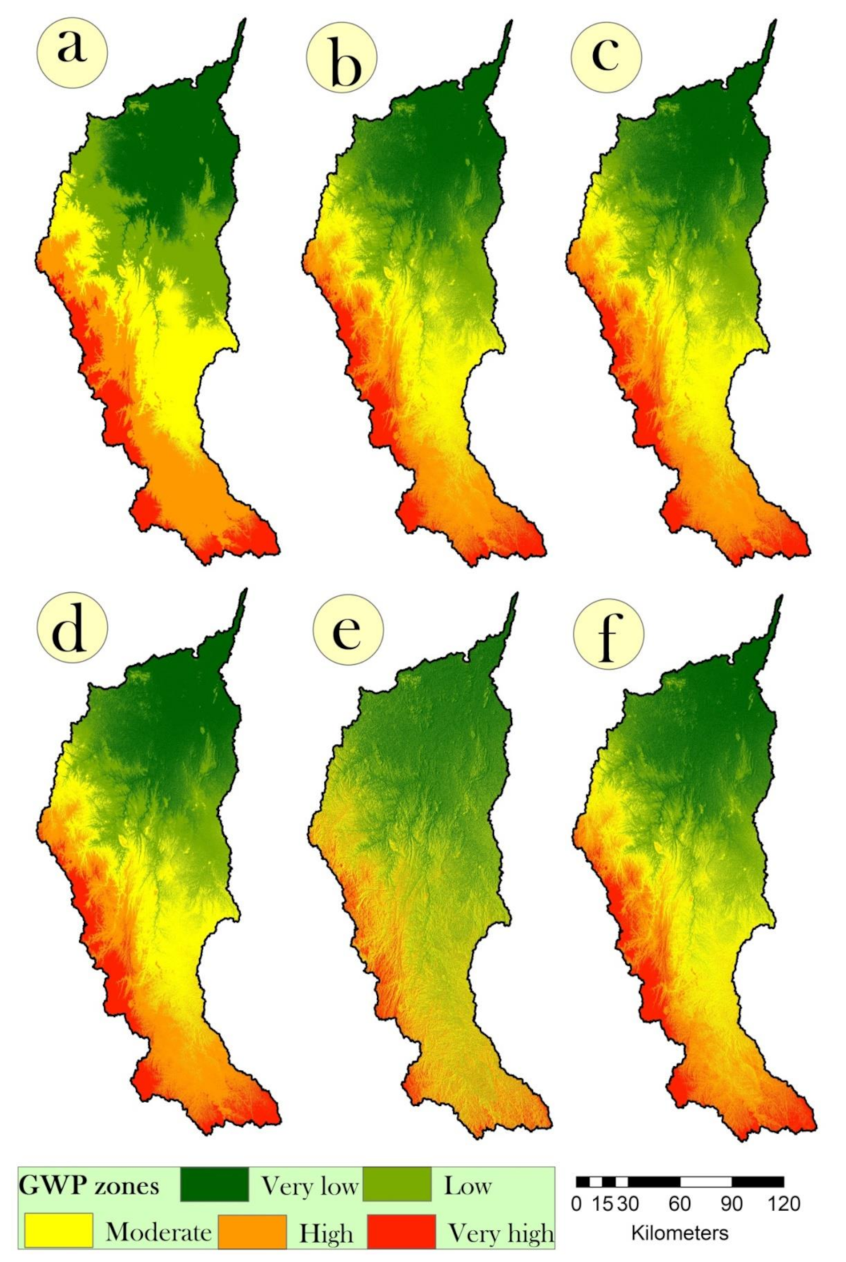
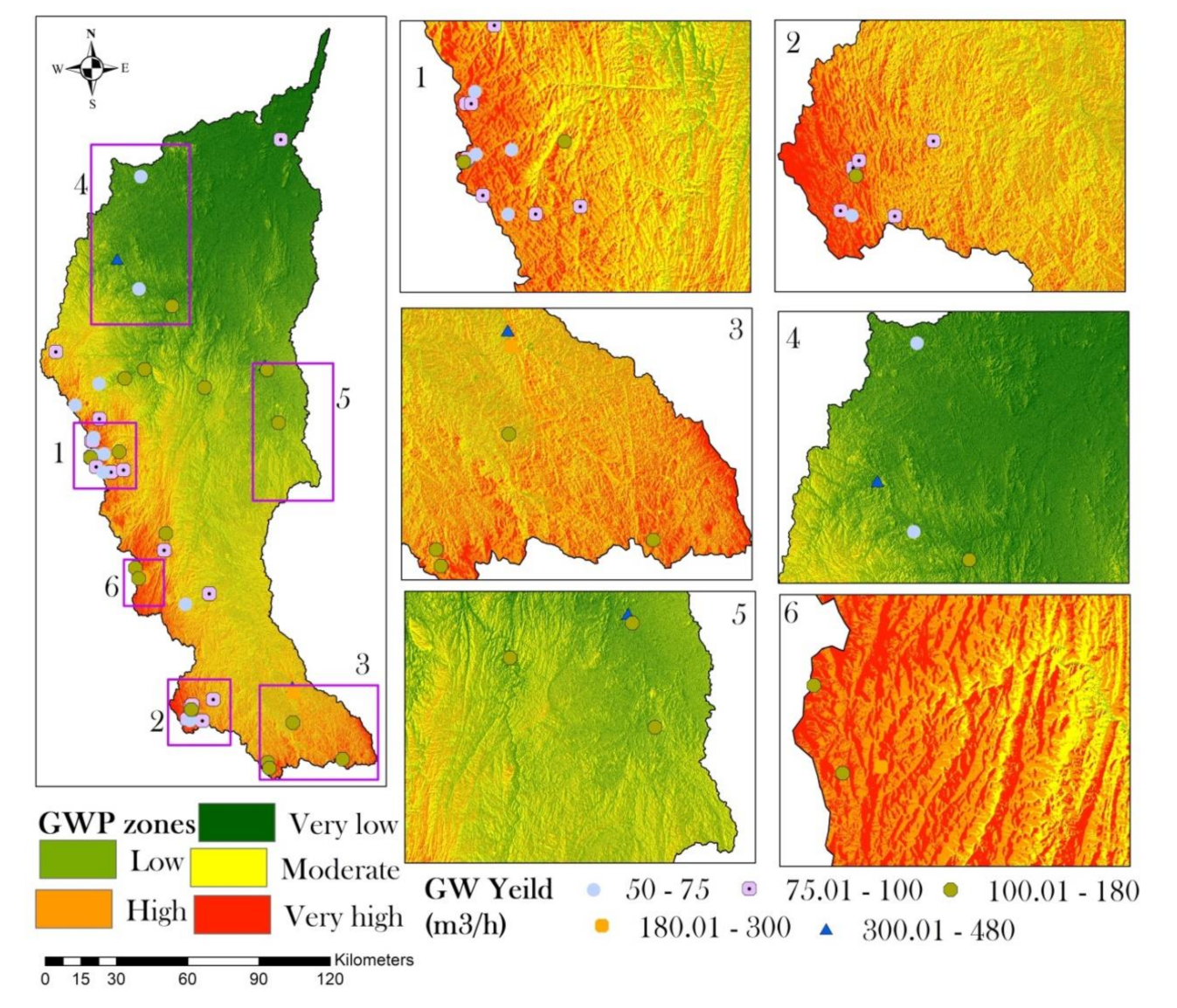
Figure 1. Study area.
Water 13 02632 g001
Figure 2. DEM derived topographic parameters, such as (a) elevation, (b) slope, (c) LS Factor, (d) TRI, (e) plan curvature, (f) profile curvature, and (g) aspect.
Water 13 02632 g002
Figure 3. DEM derived topographic and hydrologic parameters, such as (a) TPI, (b) convergence index, (c) TWI, (d) SPI, (e) flow direction, (f) flow accumulation, and (g) topographic features.
Water 13 02632 g003
Figure 4. Groundwater potentiality models based on DEM derived parameters using feature selection and fuzzy based hybrid algorithms, such as (a) AND, (b) OR, (c) GAMMA0.75, (d) GAMMA0.8, (e) GAMMA0.85, and (f) GAMMA0.9.
Water 13 02632 g004
Figure 5. Validation of the hybrid models using empirical and binormal ROC curves, (a) AND, (b) OR, (c) GAMMA0.75, (d) GAMMA0.8, (e) GAMMA0.85, and (f) GAMMA0.9.
Water 13 02632 g005
Figure 6. Sensitivity analysis for the best model (AND model) using MDA and MDG.
Water 13 02632 g006
Figure 7. Groundwater potentiality model using LR-based novel hybrid model.
Water 13 02632 g007
Figure 8. Validation of the LR-based novel hybrid model using empirical and binormal ROC curve.
Water 13 02632 g008
Table 1. Computation of area coverage under different GWP zones of hybrid models.
GWP ZonesArea (km2)
ANDORGAMMA0.75GAMMA0.8GAMMA0.85GAMMA0.9
Very high2149.952122.062112.521850.811942.182097.03
High4585.494395.944523.223644.024269.044279.91
Moderate4789.804620.934629.725071.995255.524714.25
Low4434.674835.194853.905493.595335.845181.40
Very low5323.655309.445164.215223.114480.965010.96
Publisher’s Note: MDPI stays neutral with regard to jurisdictional claims in published maps and institutional affiliations.

