Numerical Investigation of Degasification in an Electrocoagulation Reactor

Abstract

In order to enhance retention of particulate and colloidal (organic) matter, chemical coagulation (CC) is often used prior to pressure-driven membrane filtration. This combined hybrid membrane system may be a potential solution for environmental problems dealing with drinking water treatment, water reuse, and rational waste management. In this study, an EC reactor with spiral electrodes was investigated numerically, focusing on modeling with a given design/geometry configuration and boundary conditions. Two-phase flow interactions between water and hydrogen were modeled via computational fluid dynamics (CFD). Different flow rates ($\mathrm{Q}=1-1000 \mathrm{L}/\mathrm{h}$) through two batches of the watering stage (Case 1–3) and the degassing stage (Case 4–6) were simulated. The results provided information about flow characteristics such as sufficient retention time, water circulation, undesirable gas penetration into the water inlet channel, gas holdup during watering and degassing, and finally the optimal period for the degasification. Retention time decreases with increasing water velocity and thirty seconds seemed to be the optimal time with gas holdup of 0.020%, 0.028%, and 0.027%, respectively, for Case 4, Case 5, and Case 6. Another finding is that the consideration for the most abundant gas holdup for the typical BC was the smallest ratio of water to gas flow.

1. Introduction

Water scarcity is currently a serious problem in most parts of the world, owing to freshwater depletion, increasing infrastructure costs, global warming, population growth, and massive waste productions [1]. Approximately 2 million tons of industrial and agricultural wastes are discharged every day into the water and up to 80% of industrial and municipal sewage are deployed into the environment without any treatment [2,3]. Over 2 billion people already live in areas subject to water stress. In total, 45% of the world’s population i.e., approximately 3.4 billion people, lack access to safely managed sanitation facilities. According to independent assessments, the world will face a global water deficit of 40% by 2030. This situation will be worsened by global challenges such as COVID-19 and climate change [3].

Conventional wastewater treatment plants (WWTP) comprise mechanical-, biological-, and/or chemical-based purification processes. The conventional treatment of especially surface waters for drinking water purposes in drinking water treatment plants (DWTP) comprise mainly chemical-physical processes followed by disinfection prior to distribution. Both commonly use chemical coagulation (CC) in order to form larger aggregates being retained subsequently. Chemical coagulation typically involves the addition of coagulants such as iron or aluminum salts to the water in order to destabilize particles and colloids and facilitate their agglomeration to form larger flocs. Depending on process setup, organic matter can be co-precipitated and entrapped within the flocs. Therefore, coagulants and coagulant aids (e.g., acid or base for pH adjustment) are dosed and rapidly mixed in a coagulation tank, and afterwards, the flocculation aids are added and gently mixed in the flocculation tanks. The formed flocs can be effectively separated in the next process, such as sedimentation, flotation, or filtration. For instance, pressure-driven membrane filtration, such as microfiltration (MF) and ultrafiltration (UF), is state of the art technology for particle retention and widely used to treat fresh waters, waste water for recycling purposes, as a membrane bio reactor (MBR), and as a pretreatment in desalination [4].

CC is a conventional method to reduce membrane fouling, ideally being achieved by a hybrid process, combining CC with membrane filtration. The integration of coagulation with membrane filtration has two main advantages: enhanced removal of NOM molecules and reduction of membrane fouling [4,5,6,7]. For instance, the hybrid process has become a common method to comply with the legal, chemical, and microbiological requirements for drinking water [5] and in the treatment of wastewater and wastewater effluent [8]. The most recent mode in this hybrid process is to add the coagulant and coagulant aids directly into the feed stream immediately prior to the membrane process or to submerge the membrane into the water to be treated. The advantages of this in-line coagulation or submerged reactor systems are the reduced footprint, reduced retention time, and lower coagulant dose, as settle able flocs are not needed [5,8,9,10]. Generally, fouling layers formed by flocs will affect layer density, porosity, and thickness and, therefore, resistance to flow, limit pore blockage, and increasing backwash efficiency. Coagulation followed by tangential UF should gather the beneficial effects of particle growth and cross-flow velocity [6,11,12,13].

Considering CC, the main disadvantages of this treatment method are sometimes longer retention times, especially in cases where in-line coagulation is not possible. Furthermore, larger quantities of sludge and the addition of chemicals for coagulation, flocculation, and pH adjustment are to be considered, which might make the process costly. A “chemical addition free” process alternative to chemical coagulation is an electrochemical technology known as electrocoagulation (EC) [14]. EC is commonly applied in the treatment of water and industrial effluents because of its capability to remove a very wide type of pollutants, e.g., colloidal and suspended particles, heavy metal ions, and toxic organics. Moreover, EC has gained a popular attention being applicable in different water sources, not only in drinking water treatment, for instance, in produced water treatment [15], ground water [16], wastewater treatment [17], and industrial waters [18]. One of the advantages of the EC method is that coagulant chemicals are supplied electrochemically in situ and on-demand instead of a direct chemical supply [19]. One disadvantage when combined with membranes might be insufficient degasification leading to gas holdups within the membrane system. This needs to be avoided in order to maintain a stable filtration process and leads to the work presented here.

Generally, the EC process includes four steps: anode dissolution, formation of OH^– ions and H₂ at the cathode, adsorption/absorption of colloidal pollutants on coagulants, and floc removal by sedimentation or flotation [20]. The metal ions produced by electrochemical dissolution of a consumable anode (Fe and/or Al anodes) directly undergo hydrolysis in water, simultaneous cathodic reaction yields for pollutant removal either by deposition on cathode electrode or by flotation (evolution of hydrogen at the cathode) [21]. By imposing electric current between the cathode and anode, made of metals such as iron (Fe) or aluminum (Al), tiny contaminants are removed (even radioactive components) in the wastewater. The anode, e.g., iron, oxidizes and generates polyvalent metal cations directly into the water [21]:

$$\mathrm{Fe}\left(\mathrm{s}\right)\to {\mathrm{Fe}}^{2+}\left(\mathrm{aq}\right)+2{\mathrm{e}}^{-} \mathrm{or} \mathrm{Fe}\left(\mathrm{s}\right)\to {\mathrm{Fe}}^{3+}\left(\mathrm{aq}\right)+3{\mathrm{e}}^{-}.$$

On the cathode, the water molecules are reduced into hydroxyl anions and hydrogen gas [21]:

$$3{\mathrm{H}}_2\mathrm{O}+3{\mathrm{e}}^{-}\to \frac{3}{2}{\mathrm{H}}_2\left(\mathrm{g}\right)+3{\mathrm{OH}}^{-}.$$

Metal hydroxides are formed with poor solubility and readily precipitated in order to remove pollutant as a ligand (L) by surface complexation [21]:

$$\mathrm{L}\cdots {\mathrm{H}}_{\left(\mathrm{aq}\right)}+\left(\mathrm{OH}\right){\mathrm{OFe}}_{\left(\mathrm{s}\right)}\to \mathrm{L}\cdots {\mathrm{OFe}}_{\left(\mathrm{s}\right)}+{\mathrm{H}}_2\mathrm{O}.$$

Most of the important parameters that affect the EC efficiency are electric current, pH, electrode material, conductivity, treatment time, and hydrodynamics of the flow. Although some experimental works have been performed in the literature to investigate these parameters, recently, CFD has become an important tool to study fluid flow and current density inside EC reactors and to estimate complicated inherent phenomena, particularly in the case where an experimental method is restricted by technical limitations [21]. Safonyk et al. [22] numerically showed the impact of the rate of heat formation from the electrodes on the efficiency of the formation of coagulant. Song et al. [23] numerically investigated the effect of flow rate on the removal efficiency of As and Sb in an EC reactor. They found that although the increase of flow rate is advantageous to the mass transfer, it does not promote the formation of flocs and the effective combination between flocs and pollutants, leading to the decrease of the removal efficiency of As and Sb. Lu et al. [24] simulated the generation and mass transfer of soluble and insoluble hydroxides in an EC channel. They found that though (Al³⁺), H⁺, and OH⁻ are generated and accumulated at the direction of streamline, the concentration of these species increases and reaches its maximum around the inlet area, and after that, they decrease gradually to a much lower value. Al-Barakat et al. [25] numerically investigated the impacts of rotating speed of an electrode on an EC unit. They found that the increase in the rotation of an electrode enhances the removal efficiency, which reaches the maximum at 100 rpm, while at higher rotation, i.e., 150 rpm, the removal efficiency decreases gradually due to the destabilization of flocs that are formed. Vázquez et al. [26] studied the current distribution and cell hydrodynamics for the design of electrocoagulation reactors. They found that the cell geometry arrangement generates low velocity profiles between the electrodes. Delgadillo et al. [27] studied the performance evaluation of an electrochemical reactor used to reduce hexavalent chromium Cr(VI) from industrial wastewaters. The outcome of the work was that by increasing the angular velocity of the rotating ring electrodes, the Cr(VI) removal rate increases and also improves the mass transfer rate between the electrodes and the liquid.

Multiple hydrodynamic phenomena, such as channeling, internal recirculation, and dead zones, which may influence the formation of coagulations, are required to be characterized in EC reactors. Vázquez et al. [28] performed simulations to hydrodynamically characterize the EC cell performance. They showed that a higher velocity may support the removal of mud. Vázquez et al. [26] reported that when the volumetric flow increases, the area corresponding to stagnant zones decreases since the fluid starts to circulate preferentially along the cell center, and new channeling zones and recirculation regions begin to form.

Although the EC technique has many advantages compared to CC, such as less sludge generation, fewer disinfection by-products (DBP) formation, providing more efficiency in color and turbidity removal, and no chemical addition, the technique also has disadvantages, such as higher maintenance requirement for fouling control and electrode replacement. In addition, it is hard to apply this technique for low-conductivity wastewaters and complex two-phase flow hydrodynamics [21,26,27,29,30]. Considering the reactions inside the cell, two-phase flow occurs due to the hydrogen gas bubbles that are produced along the cathode and accumulate inside the electrolytic cell, which increases electrical resistance and reduces the efficiency of the process. The bubble density influences the flow hydrodynamics, which in turn affects mass transfer between pollutants, coagulant, and gas micro-bubbles, and finally directs the collision rate of coagulated particles, which results in floc formation [21]. In this context, degasification is required to get rid of gas collected inside the reactor.

The two-phase flow containing water liquid and hydrogen gas can be modeled to determine the flow characteristics. However, this phenomenon has been less investigated in ECs via CFD due to the complexity of two-phase modeling. One of the very few studies was performed by Villalobos-Lara et al. [20]. They simulated two-phase flow in a continuous rotating cylinder electrode reactor. They found that depending on the electrochemical kinetics, the conductivity of the electrolyte varies due to the formation of bubbles.

In the literature, few papers use CFD simulations of EC process and even fewer deal with its application in degasification. Therefore, this work aims to model the two-phase flow of the water and gas fluid in EC-reactor by means of CFD-tools with the Euler-Euler approach in order to describe the degassing effects at various water throughputs. Different flow rates of water and gas were investigated in two operational modes. Subsequently, the stored bubbles are modeled during watering and degassing for each case. Based on the results, the degassing period can be optimized for more effective EC operation. This is very important because it will further influence the formation and transport behavior of flocs formed in the real process. This third phase is not considered in the model as a third (solid) phase yet. This was done on purpose to focus on the area of interest. Embedding the third phase as solid particles in the model will be done in future research as well as determining the resulting fouling of the membranes.

2. Materials and Methods

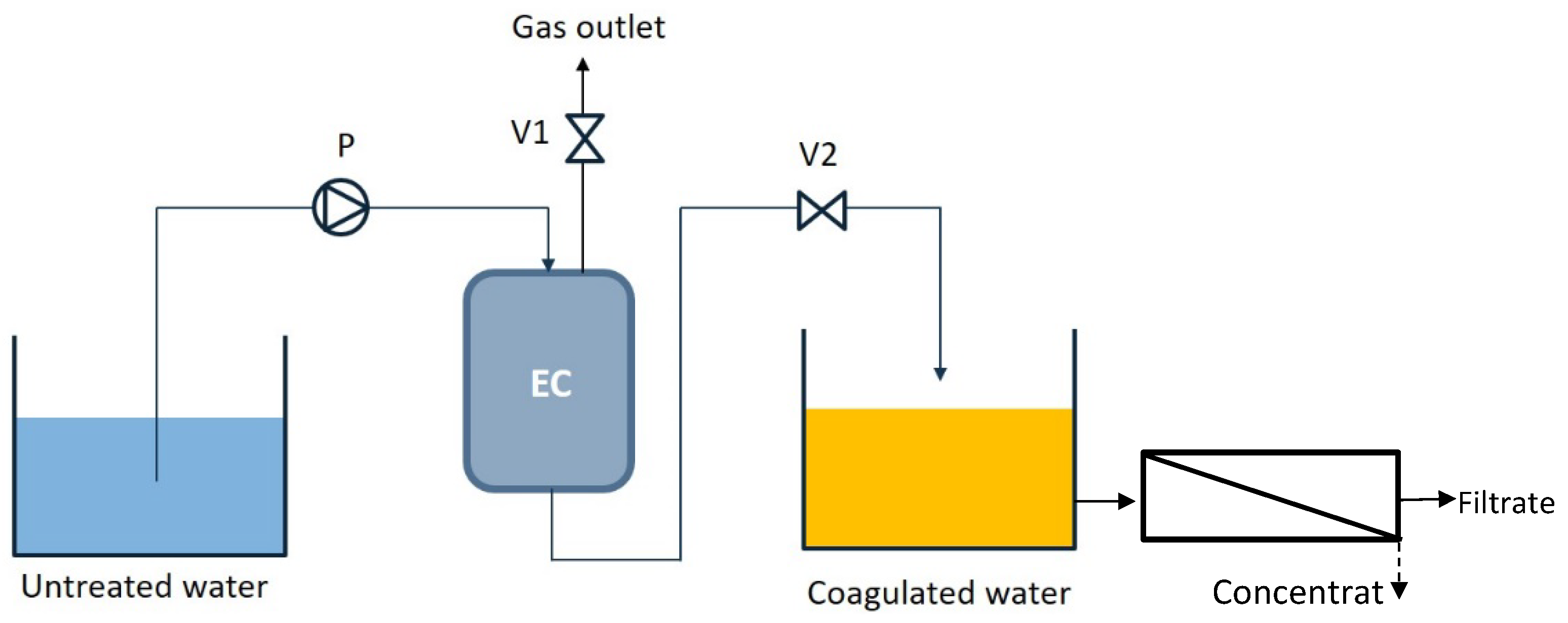
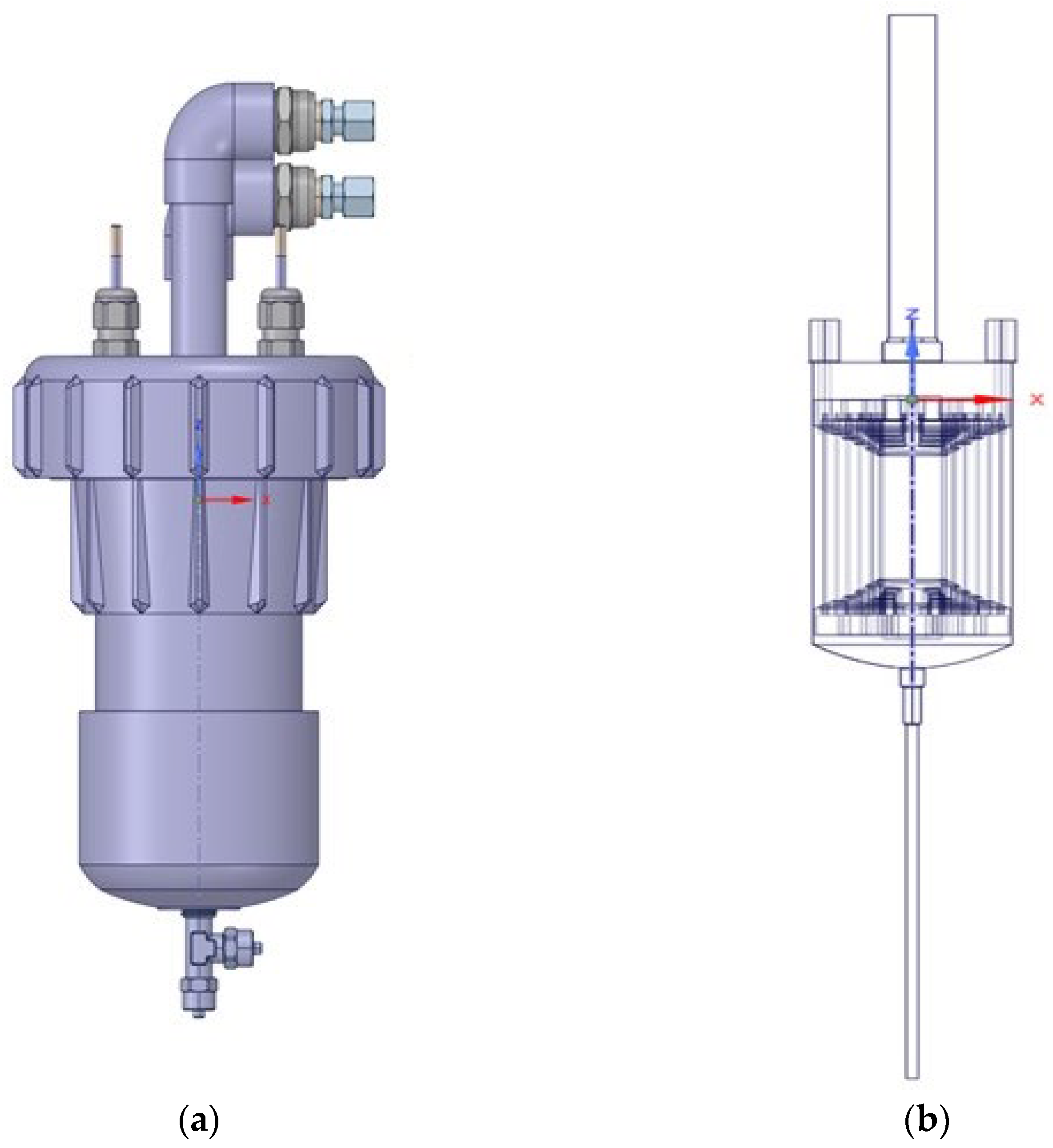
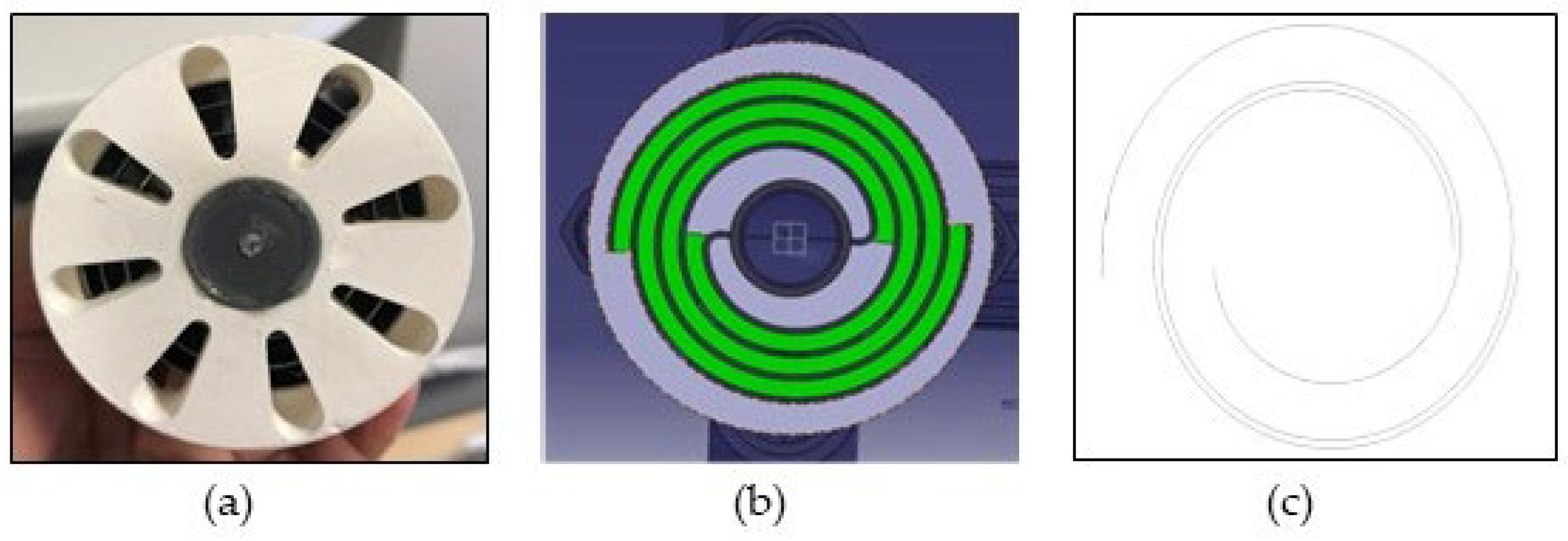
2.1. Experimental Setup

The electrocoagulation unit in Figure 1 shows the basic components during the electrocoagulation process. Two subsequent operational batches were configured in the consecutive processing with a fixed volume.

As reflected in Figure 1, the watering period starts with pump P transferring feed water from the feed water tank (untreated water) to the EC reactor through the inlet at the top. The setup was chosen in order to avoid clogging and sedimentation when just low flow velocities are applied. Then, the coagulated water leaves the reactor through the water outlet at the bottom of the reactor, and through an open water outlet valve V2, while a gas outlet valve V1 is closed. The coagulated water is collected in a tank, which might also be used to feed a membrane system. Meanwhile, gas bubbles accumulate in the reactor over the watering period. For the degassing period, the water outlet valve V2 is closed, and the gas outlet valve V1 is opened. Consequently, the deposited bubbles are gradually vented out through the gas outlet. Operating conditions of the EC reactor is shown in

Table 1. Operational conditions of the EC device for different experiments.

Parameters	Min Intervals	Max Intervals	Typical Intervals
Current density [A/m2]	1	75	25
Inlet flow [L/h]	1	1000	10
Hydrogen gas flow [g/min]	6 × 10−6	1.93 × 10−3	6.62 × 10−4
Degassing time interval [min]	15	120	60
Degassing duration [min]	0.1	2	1
Water temperature [°C]	15	25	20

, whereas six different experiments have been investigated with different flow rates in this study.

2.2. Numerical Simulation Setup

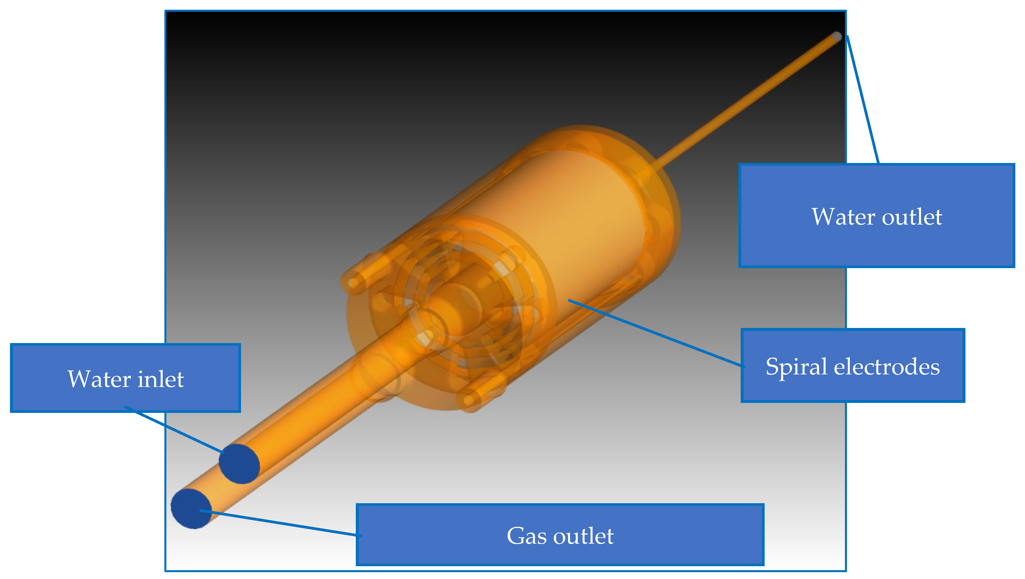
2.2.1. Geometry and Grid Generation

The EC reactor design is illustrated in Figure 2. The geometry was initially more complex with inlet and outlet bends, valves at terminals, and some small features. The EC reactor was simplified as much as possible by removing the bends and making straight pipes without connectors. The spiral electrode geometry was used without further simplification.

The spiral design was selected because (1) unlike the conventional parallel plate design, which requires complicated/multiple electrical terminal connections, a spirally wound plates only requires two terminal connections, which makes it simpler to set up, (2) a spiral design enables development of a more compact/modular design which can be housed in a cylindrical vessel/pipe, (3) a circular cross section allows more possibilities for optimal distribution of flow than rectangular cross-section, and (4) a vertical configuration allows efficient venting of hydrogen gas (avoiding unwanted accumulation in the reactor). In addition, longer pipes were attached to the water outflow for observing the pressure of the flow in the actual tubes, which means there was a height difference between the model case and the initial design. The total height of the simplified reactor (right of Figure 2) was 52 cm, but the actual device (left of Figure 2) was 28 cm high (a factor of 1.85).

The electrode configuration was a monopolar electrode in parallel connection with a helical pattern. The electrode was built using two 0.5 mm thick metal plates with a length of 97 mm and electrode spacing of 3 mm. The maximum diameter of the spirally rolled electrodes was 60 mm (see Figure 3). The effective surface area of the electrodes was 405 cm².

The fluid domain is shown in Figure 4. The diameter of the water inlet and gas outlet on the top is about d = 1.6 cm. The water outlet diameter at the bottom is d = 0.4 cm. A mesh study was performed. Different meshing tools and methods were used. Finally, the domain was discretized with tetra meshes by automatic element sizing with excellent mesh quality (average skewness 0.24), generating unstructured tetrahedral meshes with an average grid size of 1 mm. The mesh consists of 409,746 nodes and 1,930,592 elements (ratio elements/nodes ~5) (Figure 5).

Within the fluid simulation setup, the boundary conditions were defined. The water inlet was where the liquid fluid entered the geometry as fluid velocity inlet, while water exited from the water outlet as pressure boundary. The gas bubbles were produced near the cathode, and they drained out though the gas outlet.

2.2.2. Solver Setup

In this study, a two-fluid Euler-Euler model was used. In this model, specific interphase transfer terms can be modeled and the different phases are treated mathematically as interpenetrating continua. The Eulerian model solves the momentum and continuity equations for each phase with the domain pressure for all phases.

Three-dimensional simulations with a Eulerian-Eulerian model were carried out using ANSYS CFX. The two-phase model contained water liquid and hydrogen gas. Although phases were mixed at length scales much more extensive than molecular, they were assumed to be mixed at macroscopic length scales. The Euler-Euler approach was applied to solve a set of n-momentum and n-continuity equations for each phase of non-granular (fluid-fluid) flow individually.

In the fluid domain, the pure substances of water liquid and hydrogen gas (

Table 2. Material properties of the water liquid and the hydrogen gas.

Fluid Properties	Water	Hydrogen
Thermodynamic State	Liquid	Gas
Molar Mass [kg/kmol]	18.02	2.016
Density [kg/m3]	998.2	0.09
Ref. Temperature [°C]	20	20

) were prepared from available materials of the CFX library. Reference pressure (P_ref) was set at 1 atm and all relative pressures were measured to this reference pressure value.

The simulations were conducted with a water density at a constant temperature of 20 °C and hydrogen gas at standard pressure and temperature conditions. The pH-value was between 6 and 9. The water conductivity was in the range of 1000–10,000 μs/cm; typically, 5000 μs/cm was used. Although the temperatures were specified for material properties of both phases, the heat transfer was not taken into account.

In the simulations, water was defined as the continuous fluid and hydrogen gas was defined as the dispersed fluid. The shapes of hydrogen bubbles were assumed as of monodispersed spherical shapes with a diameter of 0.5 mm uniformly.

The isolated hydrogen bubbles rise in the liquid media depending on drag and buoyancy forces [31]. The density of the carrier water is much higher than the hydrogen. The full buoyancy model was appropriate in this study because it was only dependent on the density difference between the liquid and the gas phase. A source term for buoyancy calculations was added to the momentum equations, as shown in Equation (1) [32]:

$$F_b=({\rho }_{\alpha }-{\rho }_{ref})g.$$

(1)

Surface tension is a force at a free surface interface that acts to minimize the surface area of the interface. The continuum surface force model (Fs) in Equation (2) provided the surface tension force between water-phase α (primary fluid) and gas-phase β (secondary phase). It is expressed based on the adhesive force (f) [32]:

$$f_{\alpha \beta }=-{\sigma }_{\alpha \beta }{k}_{\alpha \beta }{n}_{\alpha \beta }+{\nabla }_s\sigma \to F_s=f_{\alpha \beta } \left| \nabla r_{c,\alpha \beta }\right|.$$

(2)

2.2.3. Interphase Transfer Model

Interfacial transfer of mass and momentum in the inhomogeneous model was directly proportional to the contact surface area between the two phases. The interfacial area density (A_αβ) delineated the area per unit volume between the water (phase α) and the hydrogen gas (phase β). The volumetric dimension of interfacial transfer was the inverse length, and the particle model could consider it. Equation (3) is the calculation of A_αβ relying on the area density (r) and bubble diameter (d_b) of the secondary phase (β) [32].

$$A_{\alpha \beta }=\frac{6r_{\beta }}{d_{\beta }}.$$

(3)

In the inhomogeneous model, the interphase momentum transfer occurs due to interfacial forces acting on each phase to another phase and the total forces on α-phase are denoted M_α [32].

The total drag force is expressed in terms of the dimensionless drag coefficient C_D based on Eötvös number (Eo). The number of bubbles (n_b) per unit volume is related to the interfacial density of the secondary phase (r_β) and the drag is set out by Equation (4) for two-phase flow [32]:

$$n_b=\frac{r_{\beta }}{V_b}=\frac{6r_{\beta }}{\pi d_b{}^3} \to D_{\alpha \beta }=n_b{D}_b=\frac{3}{4}\frac{C_D}{d}{r}_{\beta }{\rho }_{\alpha }\left|U_{\beta }-U_{\alpha }\right|\left(U_{\beta }-U_{\alpha }\right).$$

(4)

The lift force acts perpendicular to the direction of relative motion of the water and hydrogen gas. The Tomiyama Lift Force Model was set to model the lift force relying on Eötvös number (Eo) and maximum horizontal scale of deformable bubbles in the ellipsoidal and spherical cap regimes. The lift force, as can be seen in Equation (5), refers to the shear-induced lift force acting on a dispersed phase (d) in the presence of rotations with angular velocity (ω_c) in a continuous phase [32]:

$${\omega }_c=curl \left(U_c\right) \to F_c^L=-F_d^L=r_d{\rho }_d{C}_L\left(U_d-U_c\right)\times {\omega }_c.$$

(5)

The virtual mass force counted on relative phasic accelerations is shown in Equation (6). The virtual mass coefficient depends on shape and particle concentration, and it is 0.5 for the inviscid flow around isolated sphere particles [32]:

$$F_c^{VM}=-F_d^{VM}=r_d{\rho }_c{C}_{VM}\left(\frac{D_d{U}_d}{Dt}-\frac{D_c{U}_c}{Dt}\right).$$

(6)

2.2.4. Turbulence Model

The Navier–Stokes equations represent the motions of fluid flows. Through time-averaged terms, the Reynolds Averaged Navier–Stokes (RANS) equation is shown in Equation (7). The last term of the equation is Reynolds stress, which has to be modeled with the RANS equation [32]:

$$\frac{\partial U_i}{\partial t}+U_j\frac{\partial U_i}{\partial x_j}=\frac{1}{\rho }\frac{\partial }{\partial x_j}\left(-P·{\delta }_{ij}+2\mu S_{ij}-\rho \overline{u_i{}^{\prime }{u}_j{}^{\prime }}\right).$$

(7)

$$-\rho \overline{u_i{}^{\prime }{u}_j{}^{\prime }}=2\mu \left(\frac{\partial U_i}{\partial x_j}+\frac{\partial U_j}{\partial x_i}-\frac{2}{3}\frac{\partial U_k}{\partial x_k}{\delta }_{ij}\right)-\frac{2}{3}\rho k{\delta }_{ij}$$

(8)

A zero-equation model was implemented for hydrogen gas, and a constant turbulent eddy viscosity was calculated for the entire flow domain without additional transport equations [33]. The zero-equation model in ANSYS CFX (see Equation (9)) uses an algebraic equation to determine a constant turbulent eddy viscosity [32]:

$$v_{td}=\frac{v_{tc}}{P{r}_t} \leftrightarrow {\mu }_{td}=\frac{{\rho }_d}{{\rho }_c} \frac{{\mu }_{tc}}{P{r}_t}.$$

(9)

Two-equation turbulence models are broadly used, as they offer a genuine compromise between numerical effort and computational accuracy. The turbulent viscosity is modeled as turbulent velocity and turbulent length scale. The Shear Stress Transport (SST) was applied for modeling the turbulence of the liquid, and it was the most prominent two-equation models in this area of κ-ω based models of Menter [33]. For the κ-ω model, the turbulent viscosity is modeled in Equation (10). The transport equations for κ and ω are revealed respectively in Equations (11) and (12). The turbulent phase is assumed to take a similar form to the single-phase transport equations [32].

$${\mu }_{t\alpha }=c_{\mu }{\rho }_{\alpha }\frac{{\kappa }_{\alpha }^2}{{\omega }_{\alpha }},$$

(10)

$$\frac{\partial }{\partial t}\left(r_{\alpha }{\rho }_{\alpha }{\kappa }_{\alpha }\right)+\nabla ·\left(r_{\alpha }\left({\rho }_{\alpha }{U}_{\alpha }{\kappa }_{\alpha }-\left(\mu +\frac{{\mu }_{t\alpha }}{{\sigma }_k}\right)\nabla {\kappa }_{\alpha }\right)\right)=r_{\alpha }\left(P_{\alpha }-{\rho }_{\alpha }{\omega }_{\alpha }\right)+T_{\alpha \beta }{}^{\left(k\right)},$$

(11)

$$\frac{\partial }{\partial t}\left(r_{\alpha }{\rho }_{\alpha }{\omega }_{\alpha }\right)+\nabla ·\left(r_{\alpha }\left({\rho }_{\alpha }{U}_{\alpha }{\omega }_{\alpha }-\left(\mu +\frac{{\mu }_{t\alpha }}{{\sigma }_{\omega }}\right)\nabla {\omega }_{\alpha }\right)\right)=r_{\alpha }\frac{{\omega }_{\alpha }}{{\kappa }_{\alpha }}\left(C_{\omega 1}{P}_{\alpha }-C_{\omega 2}{\rho }_{\alpha }{\omega }_{\alpha }\right)+T_{\alpha \beta }{}^{\left(\omega \right)}.$$

(12)

Bigger bubbles in the dispersed hydrogen phase tended to increase turbulence in the continuous water due to the presence of wakes behind the bubbles, and it introduced bubble-induced turbulence. The Sato-enhanced eddy viscosity model could be used to improve the turbulence transfer of the continuous phase. Bubble-induced turbulence based on Sato [34], as shown in Equation (13), was utilized, where µ_ts is the usual shear-induced eddy viscosity, µ_tp is additional bubble-induced eddy viscosity, and variable C_µp has a value of 0.6 [32]:

$${\mu }_{tp}=C_{\mu p}{\rho }_c{r}_d{d}_p\left|U_d-U_c\right| \to {\mu }_{tc}={\mu }_{ts}+{\mu }_{tp }$$

(13)

3. Results and Discussion

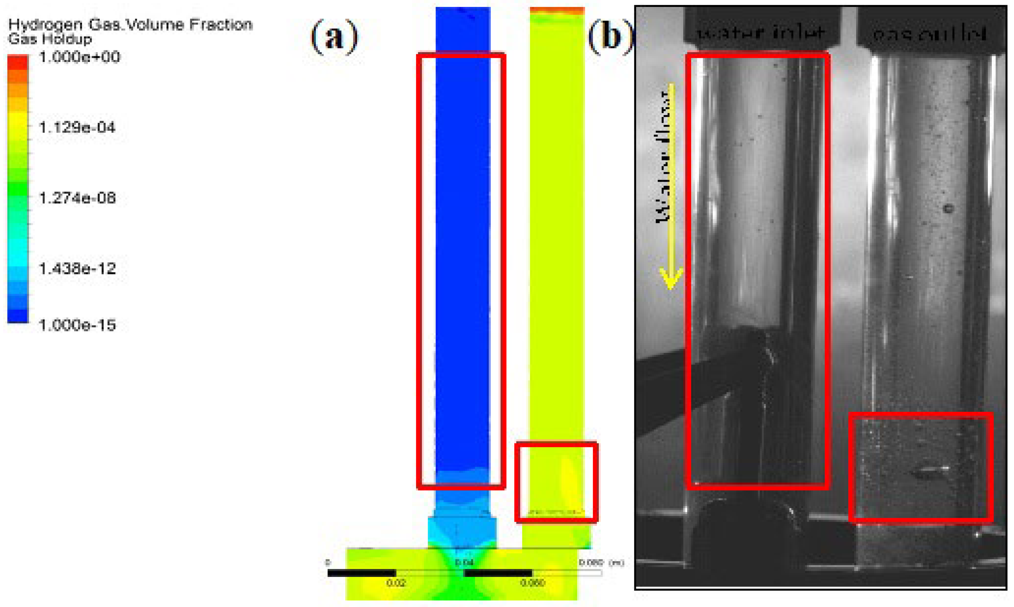
3.1. Verification and Validation

The types of the boundary conditions (see Figure 4) were defined for watering and degassing. Six cases according to the corresponding experiments were modeled: Case 1–3 was corresponding to the watering stage and Case 4–6 was for the degassing. The cases had different boundary conditions (BCs), whose minimum values were Case 1 and 4, typical values were Case 2 and 5, and maximum values were Case 3 and 6. The BCs of all cases are specified in

Table 3. Boundary conditions for Case 1–6 with the water inlet, water outlet, spiral cathode, and gas outlet.

BCs	Case 1	Case 2	Case 3	Case 4–6
Water inlet	$\dot{m}=0.00028 \mathrm{kg}/\mathrm{s}$	$\dot{m}=$ 0.00278 $\mathrm{kg}/\mathrm{s}$	$\dot{m}=$ 0.27778 $\mathrm{kg}/\mathrm{s}$	$\dot{m}=0 \mathrm{kg}/\mathrm{s}$
Water outlet	$P_{rel}=0 \mathrm{bar}$	$P_{rel}=0 \mathrm{bar}$	$P_{rel}=0 \mathrm{bar}$	$\dot{m}=0 \mathrm{kg}/\mathrm{s}$
Spiral Cathode	$\dot{m}={10}^{-7} \mathrm{kg}/\mathrm{s}$	$\dot{m}=1.1 \times {10}^{-7} \mathrm{kg}/\mathrm{s}$	$\dot{m}=3.2 \times {10}^{-7} \mathrm{kg}/\mathrm{s}$	$\dot{m}=0 \mathrm{kg}/\mathrm{s}$
Gas outlet	$\dot{m}=0 \mathrm{kg}/\mathrm{s}$	$\dot{m}=0 \mathrm{kg}/\mathrm{s}$	$\dot{m}=0 \mathrm{kg}/\mathrm{s}$	degassing

. The water is injected by the water inlet boundary, while the gas bubbles are uniformly injected at the spiral cathode boundary (wall).

The time dependence of the flow could be specified as either steady-state or transient. The flow for the watering stages (Case 1–3) were assumed to be steady-state because the operation time was too long (ca. 2 h), and the steady-state condition has been reached. The transient model was set for the degassing stages (Case 4–6) for 2 min due to the changing boundary conditions.

The automatic time scale was set for the watering stage. The adaptive time step was allocated for degassing to track the progress of real-time based on the RMS of Courant Friedrichs Lewy (CFL) [35]. During transient simulations, the time steps were adaptively chosen to reach RMS_CFL = 1, and they were sufficiently small.

The model was validated with experimental data from tests with a bench-scale EC reactor fabricated with the same modified design shown in Figure 2. For this test, the water inlet and gas outlet pipes were extended to 10 cm and made up of transparent PVC material to enable visual observation of the movement of gas bubbles through the pipes. A high-speed camera (Photron Mini UX100) was focused on the two pipes and recorded videos with 1000 fps (frame per second) with full HD resolution (1080p). The EC was operated at the same settings as Case 2 in Table 3. The simulated retention time with normal velocity was predicted to be 55 s, which matched with the experimental duration of 55 s.

Figure 6 shows the modeled gas volume fractions on the left and the experimental gas holdup on the right for the maximum flow rate. The simulation authenticates that the gas population in the channel of the gas outlet is much larger than at the water inlet. The gas accretion at the bottom of the gas pipe is noticed in the experiment and also in the simulation, as can be seen in Figure 6.

3.2. Hydraulic Retention Time

The water streamline illustrates the water flow starting at the water inlet, as shown in Figure 7. The water enters the reactor from the water inlet, and then flows through the electrodes; finally, the treated water exits the domain from the water outlet. The water flow is disturbed by the opposite movement of the gas. However, the diameter variation and obstacles in front of the water originated the irregular flow.

The time that the water resided in the reactor (Hydraulic Retention Time (HRT)) depends on the flow rate. The retention times were indicated in

Table 4. Hydraulic retention times.

	Case 1	Case 2	Case 3
Retention time [s] water velocity	486	67	8
Retention time [s] superficial water velocity	473	55	8

and they were 468, 67, and 8 s for Case 1, Case 2, and Case 3, respectively. Nevertheless, the residence time with the superficial velocity is shorter due to the neglection of the gas effects. The hydrogen bubbles intended to rise naturally, and they were deposited around the cathode and at the gas outlet.

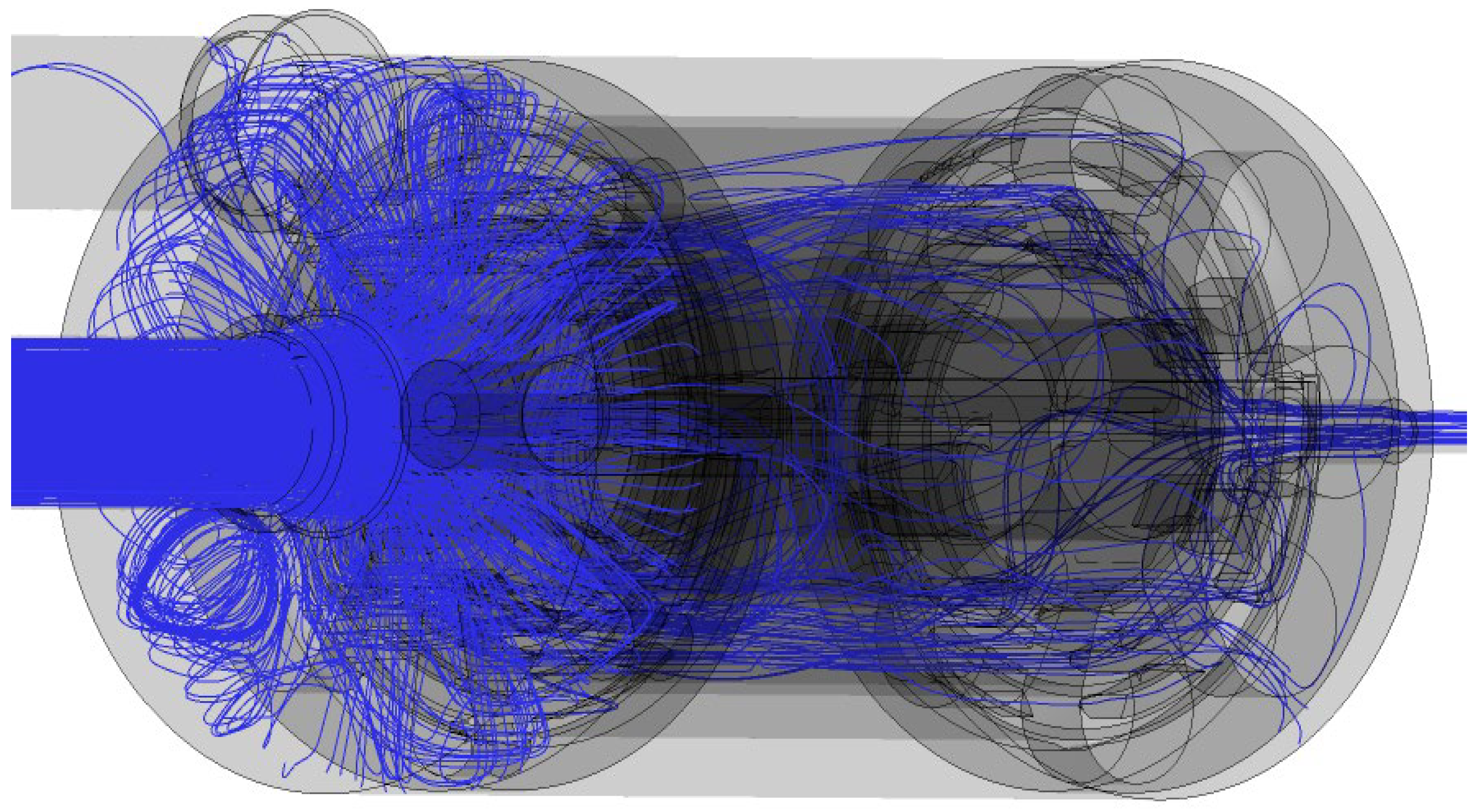
3.3. Velocity Vectors

Figure 8 shows the water flow using velocity vector plots in the central plane. The contour of the water velocity in the inflow pipe was equal with the initial water inlet velocity for Case 3. The vectors showed a downward directed flow (Case 3), but the water velocity vectors in Case 1 and 2 were bewildered by the gas flow.

3.4. Gas Holdup

The gas holdup is the most significant parameter in industrial bubble flows, and it influences the separation efficiency. The electrolysis commenced gas filling in the EC reactor, and the hydrogen bubbles reached the peak within 3 s. The gas holdups at the beginning were 0%, and they showed to be filled up to 0.3% (Case 1), 3.76% (Case 2), and 0.22% (Case 3) at the end of the watering stage. The speculation for the most abundant gas holdup for the typical BC was the smallest ratio of water flow to gas flow. After 2 min of degassing, Case 4–6 reached approximately 0.02% of gas holdup. Figure 9 shows the gas volume fractions before degassing (i.e., after watering) and after degassing.

For optimization of degassing, the whole period of the degasification has been investigated to find sufficient time for this purpose. Thirty seconds seemed to be the most appropriate duration, with a gas holdup of 0.020%, 0.028%, and 0.027%, respectively, for Case 4, Case 5, and Case 6.

Table 4 quantifies the important numbers of Figure 10 for evaluation of the lengths of the degassing period. The values of gas holdups before degassing are equal to the gas volume fractions at the end of the watering stage. To compare with the final time after two minutes, the optimal period for degassing is 30 s with a 90% progress, as shown in Figure 10 and

Table 5. Gas holdup while degassing at t = 0 s, t = 30 s, and t = 120 s for different flow rates.

	Case 4	Case 5	Case 6
Gas holdup [%] before degassing	0.3	3.76	0.22
Gas holdup [%] after 30 s	0.020	0.028	0.027
Gas holdup [%] after 120 s	0.019	0.020	0.020

.

4. Conclusions

For the removal of stabilized particles smaller than one micrometer, the electrocoagulation method is an effective way for water treatment. The geometry of an EC reactor with spiral electrodes was used for numerical simulations. The simulations consist of six cases with different flow rates. The results showed that lower water flow rates correspond to higher retention times. Water circulations correspond to the solid interiors of the reactor and the opposite gas motion. It was also found that gas penetration into the water inlet channel depends on velocity magnitudes in the vertical direction. The experiment and the numerical simulation showed a large gas holdup around the cathode and in the gas outlet. The current study worked in a batch mode with two watering and degassing stages, and each batch commenced after the other one. One proposal for design improvement is that the future design should cover continuous watering and degassing stages simultaneously. The bubble size distribution was assumed to be uniform with 0.5 mm, but in reality, the bubbles had different bubble diameters. Therefore, a polydispersed model has to be used with several categories of bubble sizes in future work. In addition, the effects of bubble coalescence and breakage have not been applied in this study. Wire-mesh sensors could be applicable to measure the volume and bubble size fractions.

However, the formed flocs which are formed in the real process are not considered in the model as a third (solid) phase yet. This was done on purpose to focus on the area of interest. Embedding the third phase as solid particles in the model will be done in future research as well as determining the resulting fouling of the membranes.

References

1. Worthington, A.C.; Hoffman, A.M. A State of the Art Review of Residential Water Demand Modelling. In School of Accounting & Finance, University of Wollongong, Working Paper 6; 2007; Available online: https://ro.uow.edu.au/accfinwp/6/ (accessed on 12 February 2021).
2. Ross, N. World Water Quality Facts and Statistics—World Water Day 2010’; Pacific Institute: Oakland, CA, USA, 2010; Available online: https://pacinst.org/publication/world-water-quality-facts-and-statistics-world-water-day-2010/ (accessed on 12 February 2021).
3. UNESCO. World Water Assessment Programme. 14 September 2020. Available online: https://en.unesco.org/wwap (accessed on 3 June 2021).
4. Tambo, N.; Ogasawara, K. Physical and Chemical Separation in Water and Wastewater Treatment; IWA Publishing: London, UK, 2020. [Google Scholar]
5. Keucken, A.; Heinicke, G.; Persson, K.M.; Köhler, S.J. Combined Coagulation and Ultrafiltration Process to Counteract Increasing NOM in Brown Surface Water. Water 2017, 9, 697. [Google Scholar] [CrossRef] [Green Version]
6. Yu, W.; Liu, M.; Zhang, X.; Graham, N.; Qu, J. Effect of pre-coagulation using different aluminium species on crystallization of cake layer and membrane fouling. NPJ Clean Water 2019, 2, 17. [Google Scholar] [CrossRef] [Green Version]
7. Lerch, A.; Panglisch, S.; Buchta, P.; Tomita, Y.; Yonekawa, H.; Hattori, K. Direct river water treatment using coagulation/ceramic membrane microfiltration. Desalination 2005, 179, 41–50. [Google Scholar] [CrossRef]
8. Aly, S.A.; Anderson, W.B.; Huck, P.M. In-line coagulation assessment for ultrafiltration fouling reduction to treat secondary effluent for water reuse. Water Sci. Technol. 2020, 83, 284–296. [Google Scholar] [CrossRef] [PubMed]
9. Ho, J.S.; Ma, Z.; Qin, J.; Sim, S.H.; Toh, C.-S. Inline coagulation–ultrafiltration as the pretreatment for reverse osmosis brine treatment and recovery. Desalination 2015, 365, 242–249. [Google Scholar] [CrossRef]
10. Wang, J.; Wang, X. Ultrafiltration with in-line coagulation for the removal of natural humic acid and membrane fouling mechanism. J. Environ. Sci. 2006, 18, 880–884. [Google Scholar] [CrossRef]
11. Arkhangelsky, E.; Lerch, A.; Uhl, W.; Gitis, V. Organic fouling and floc transport in capillaries. Sep. Purif. Technol. 2011, 80, 482–489. [Google Scholar] [CrossRef]
12. Lerch, A. Fouling layer formation by flocs in inside-out driven, horizontal aligned capillary ultrafiltration membranes. Desalination 2011, 283, 131–139. [Google Scholar] [CrossRef]
13. Barbot, E.; Moustier, S.; Bottero, J.Y.; Moulin, P. Coagulation and ultrafiltration: Understanding of the key parameters of the hybrid process. J. Membr. Sci. 2008, 325, 520–527. [Google Scholar] [CrossRef]
14. Harif, T.; Khai, M.; Adin, A. Electrocoagulation versus chemical coagulation: Coagulation/flocculation mechanisms and resulting floc characteristics. Water Res. 2012, 46, 3177–3188. [Google Scholar] [CrossRef] [PubMed]
15. Manilal, A.M.; Soloman, P.A.; Basha, C.A. Removal of Oil and Grease from Produced Water Using Electrocoagulation. J. Hazard. Toxic Radioact. Waste 2020, 24. Available online: https://ascelibrary.org/doi/abs/10.1061/%28ASCE%29HZ.2153-5515.0000463 (accessed on 3 June 2021). [CrossRef]
16. Amarine, M.; Lekhlif, B.; Sinan, M.; El Rharras, A.; Echaabi, J. Treatment of nitrate-rich groundwater using electrocoagulation with aluminum anodes. Groundw. Sustain. Dev. 2020, 11, 100371. Available online: https://www.sciencedirect.com/science/article/abs/pii/S2352801X19302991 (accessed on 3 June 2021). [CrossRef]
17. Tahreen, A.; Jami, M.S.; Ali, F. Role of electrocoagulation in wastewater treatment: A developmental review. J. Water Process. Eng. 2020, 37, 101440. [Google Scholar] [CrossRef]
18. Vepsäläinen, M.; Sillanpää, M. Electrocoagulation in the treatment of industrial waters and wastewaters. In Advanced Water Treatment; Elsevier: Amsterdam, The Netherlands, 2020; pp. 1–78. [Google Scholar] [CrossRef]
19. Ghernaout, D.; Elboughdiri, N. An Insight in Electrocoagulation Process through Current Density Distribution (CDD). Open Access Libr. J. 2020, 7, 98473. [Google Scholar] [CrossRef]
20. Villalobos-Lara, A.D.; Pérez, T.; Uribe, A.R.; Alfaro-Ayala, J.A.; de Jesús Ramírez-Minguela, J.; Minchaca-Mojica, J.I. CFD simulation of biphasic flow, mass transport and current distribution in a continuous rotating cylinder electrode reactor for electrocoagulation process. J. Electroanal. Chem. 2020, 858, 113807. [Google Scholar] [CrossRef]
21. Hakizimana, J.N.; Gourich, B.; Chafi, M.; Stiriba, Y.; Vial, C.; Drogui, P.; Naja, J. Electrocoagulation process in water treatment: A review of electrocoagulation modeling approaches. Desalination 2017, 404, 1–21. [Google Scholar] [CrossRef]
22. Safonyk, A.; Prysiazhniuk, O. Modeling and Simulation in Engineering Modeling of the Electrocoagulation Processes in Nonisothermal Conditions. Model. Simul. Eng. 2019, 2019, e9629643. [Google Scholar] [CrossRef]
23. Song, P.; Song, Q.; Yang, Z.; Zeng, G.; Xu, H.; Li, X.; Xiong, W. Numerical simulation and exploration of electrocoagulation process for arsenic and antimony removal: Electric field, flow field, and mass transfer studies. J. Environ. Manag. 2018, 228, 336–345. [Google Scholar] [CrossRef] [PubMed]
24. Lu, J.; Wang, Z.; Ma, X.; Tang, Q.; Li, Y. Modeling of the electrocoagulation process: A study on the mass transfer of electrolysis and hydrolysis products. Chem. Eng. Sci. 2017, 165, 165–176. [Google Scholar] [CrossRef]
25. Al-Barakat, H.S.; Matloub, F.K.; Ajjam, S.K.; Al-Hattab, T.A. Modeling and Simulation of Wastewater Electrocoagulation Reactor. IOP Conf. Ser.: Mater. Sci. Eng. 2020, 871, 012002. [Google Scholar] [CrossRef]
26. Vázquez, A.; Nava, J.L.; Cruz, R.; Lázaro, I.; Rodríguez, I. The importance of current distribution and cell hydrodynamic analysis for the design of electrocoagulation reactors. J. Chem. Technol. Biotechnol. 2014, 89, 220–229. [Google Scholar] [CrossRef]
27. Martinez-Delgadillo, S.; Mollinedo-Ponce, H.; Mendoza-Escamilla, V.; Gutiérrez-Torres, C.; Jiménez-Bernal, J.; Barrera-Diaz, C. Performance evaluation of an electrochemical reactor used to reduce Cr(VI) from aqueous media applying CFD simulations. J. Clean. Prod. 2012, 34, 120–124. [Google Scholar] [CrossRef]
28. Vázquez, A.I.; Almazán, F.J.; Cruz-Diaz, M.; Delgadillo, J.A.; Lázaro, M.I.; Ojeda, C.; Rodríguez, I. Characterization of a Multiple-Channel Electrochemical Cell by Computational Fluid Dynamics (CFD) and Residence Time Distribution (RTD). ECS Trans. 2010, 29, 215. [Google Scholar] [CrossRef]
29. Emamjomeh, M.M.; Sivakumar, M. Review of pollutants removed by electrocoagulation and electrocoagulation/flotation processes. J. Environ. Manag. 2009, 90, 1663–1679. [Google Scholar] [CrossRef] [PubMed]
30. Han, M.; Song, J.; Kwon, A. Preliminary investigation of electrocoagulation as a substitute for chemical coagulation. Water Supply 2002, 2, 73–76. [Google Scholar] [CrossRef]
31. Talaia, M.A.R. Terminal Velocity of a Bubble Rise in a Liquid Column. World Acad. Sci. Eng. Technol. 2007, 28, 264–268. [Google Scholar]
32. ANSYS CFX. ANSYS CFX 19.2 Documentation. 2019. Available online: https://ansyshelp.ansys.com/ (accessed on 29 November 2019).
33. Menter, F. Zonal Two Equation k-w Turbulence Models For Aerodynamic Flows. In Proceedings of the 23rd Fluid Dynamics, Plasmadynamics, and Lasers Conference, Orlando, FL, USA, 6–9 July 1993; Available online: https://arc.aiaa.org/doi/10.2514/6.1993-2906 (accessed on 19 May 2021).
34. Sato, Y.; Sekoguchi, K. Liquid velocity distribution in two-phase bubble flow. Int. J. Multiph. Flow 1975, 2, 79–95. [Google Scholar] [CrossRef]
35. de Moura, C.A.; Kubrusly, C.S. (Eds.) The Courant–Friedrichs–Lewy (CFL) Condition: 80 Years after Its Discovery; Birkhäuser: Basel, Switzerland, 2013. [Google Scholar] [CrossRef]
Figure 1. Schematic diagram of the electrocoagulation unit with optional membrane filtration.
Water 13 02607 g001
Figure 2. Shaded original design (a) and simplified EC reactor (b).
Water 13 02607 g002
Figure 3. The spiral electrodes viewed: (a) through the end caps (left), (b) the effective electrocoagulation zone shaded in green (middle), and (c) the spiral electrodes geometry (right).
Water 13 02607 g003
Figure 4. Boundary conditions of the EC-reactor with water inlet, water outlet, spiral cathode, and gas outlet.
Water 13 02607 g004
Figure 5. Domain discretization by tetrahedral cells.
Water 13 02607 g005
Figure 6. Qualitative visual comparison of bubble accumulation in the simulation (a) and the experiment (b).
Water 13 02607 g006
Figure 7. Water flow shown with streamlines during the watering period (left top, rotated 90°).
Water 13 02607 g007
Figure 8. Vectors of water velocity: (a) Case 3 and (b) Case 2 while watering.
Water 13 02607 g008
Figure 9. Gas volume fractions before (a) and after (b) degasification.
Water 13 02607 g009
Figure 10. Gas holdups in logarithmic scale during 120 s degassing for different flow rates and current densities.
Water 13 02607 g010