1. Introduction
Groundwater is an indispensable natural resource to provide the necessary water supply for the irrigation system and industry, as well as to support the health and survival of the natural ecosystem in arid and semi-arid regions where surface water is scarce [
1,
2,
3]. However, with groundwater being over-exploited and potentially facing a risk of depletion, the sustainable management of the groundwater resources becomes a crucial task in these regions [
4,
5,
6]. Moreover, in areas where groundwater is used for irrigation supply, water allocation is usually scheduled ahead of time according to the projected water availability [
7]. For this purpose, the practical forecast of groundwater resources is quite essential.
The groundwater level (GWL) is a key parameter required to quantify groundwater resources. The accurate and reliable prediction of the GWL is fundamental for evaluating the groundwater availability and effective management of the irrigation schedules [
8,
9]. Similar to other arid regions globally, the Jiuquan basin has experienced a general groundwater deterioration in both storage and sustainability [
10]. Well-known for lying on the Silk Road and being a significant irrigated agricultural area of northwest China, the area urgently needs sustainable groundwater management. To achieve this, the accurate GWL forecast is of critical importance. However, detailed predictions for the region are still lacking.
Generally, the physically based models have traditionally been primary tools for GWL simulation [
11,
12,
13]. However, the highly nonlinear, non-stationary and relatively complex hydrological system, the need of lots of hydrogeological data as well as the proper initial and boundary conditions bring plenty of difficulties in the characterization of the real hydrological system, and thus threaten the accuracy and the popularization of these models [
14,
15]. With the rapid growth of the data-based methods (mainly machine learning models), conventional algorithms such as the artificial neural network (ANN), the support vector machine (SVM), the extreme learning machine (ELM), the adaptive neuro-fuzzy inference system (ANFIS) and genetic programming (GP) have become viable techniques for groundwater forecasting owing to the greater simplicity in design and flexibility [
16,
17]. A comprehensive and explicit review of the machine learning application in GWL modeling can be found in Rajaee et al. [
18]. However, the simplified architecture limits their ability to perform deeper feature extraction and they continue to be regarded as ‘shallow learning’ models as well. The dependable simulating and predicting GWL (including evaluating the underlying uncertainties) remains relatively challenging.
It is not until recently that the deep learning models (as a new class of machine learning models) have attracted great research attention, especially in pattern recognition, signal processing, time series analysis and complex modelling tasks such as image processing [
19,
20,
21]. In terms of groundwater modeling, Zhang et al. [
22] developed a Short-Term Long Memory (LSTM) network for the groundwater table, concluding its robust learning capability to replicate the patterns of the groundwater table. Compared with the other fields (e.g., solar radiation modeling), the application of the deep learning models in groundwater prediction is deficient.
In this study, one specific type of the deep learning model of interest is the deep belief network (DBN), which exhibits an outstanding ability to extract the inherent pairwise input(s)-target features from the lowest to the highest level [
23,
24,
25]. Considering the complexity and nonlinearity of the GWL fluctuations, the DBN algorithm could be an appropriate choice. However, the utility of the DBN in GWL forecasting is few reported, urging the necessity to explore its potentiality in this field.
In light of the stochastic and non-stationary characteristics of the GWL fluctuations, effective data pre-processing tools such as wavelet transform (WT) are usually advocated. Successful applications of WT have been conducted in hydrological forecasting [
26,
27,
28,
29]. However, the excessive dependency on the selection of the mother wavelet and the decomposition level make the WT neither prior knowledge-based nor a regular or automated tool [
18]. Recently, the Empirical Mode Decomposition (EMD), Ensemble EMD (EEMD) and their improved version (e.g., Complete Ensemble EMD with Adaptive Noise, CEEMDAN) have been proposed as alternatives. Compared with EMD and EEMD, the CEEMDAN algorithm reconstructs the original signal completely and noiselessly without trial-and-error processes. This outstanding advantage results in its feasible application in several hydrological prediction problems, such as the prediction of runoff, soil water, wind speed and others [
30,
31,
32,
33,
34]. Comparatively speaking, the CEEMDAN model seems to outperform the other two models. Despite the achieved acceptable results of the CEEMDAN algorithm, no prior study in multi-timescale GWL forecasting has been carried out to the best of the authors’ knowledge.
Although the machine learning models’ coupling data pre-processing techniques (e.g., EMD, EEMD or CEEMDAN) have achieved more accuracy than the traditional models, limitations still exist in practical usage. For example, the EMD, EEMD or the CEEMDAN algorithm decomposes a complex series into the intrinsic mode functions (IMFs) and residual component (Res), which may lead to the loss of vital information since some of the resulting IMFs become the unsystematic and disorderly parts among the other IMFs, and consequently, are likely to deteriorate the forecasting accuracy.
To solve this problem, solutions either to eliminate the IMFs that contained highly perturbing frequencies signals [
35] or to build a model with a two-phase decomposition system [
36,
37,
38,
39] are commonly accepted. The removal of the irrelevant IMFs and selecting the most influential features are thus considered necessary steps when establishing any EMD, EEMD and CEEMDAN hybrid hydrological forecasting models [
40,
41]. Normally, the feature selection (FS) process is achieved collectively using the autocorrelation function (ACF) and the partial autocorrelation (PACF) method. Nevertheless, being purely linear, the ACF and PACF procedures cannot capture the nonlinear relationship between the target and the exploratory variables. Regarding the superior capability of machine learning in feature selection, the genetic algorithm (GA) is able to deduce the nonlinear relationships through the heuristic search and optimization techniques [
42]. This study, therefore, attempts to integrate for the first time, the CEEMDAN decomposition method and the GA feature selection method into a deep belief network model for GWL forecasting.
In addition, in practical GWL forecasting applications, the machine learning models are often applied without considering the uncertainties. Although a majority of the EMD-, EEMD- and CEEMDAN (or WT-equivalent)-based deep learning models appear to improve the forecasting capability, the issue of uncertainty is often neglected. Moreover, the deterministic prediction may not be sufficient to describe the inherent uncertainties. In this respect, the quantile regression (QR) method, widely used for conditional quantiles estimation, can be a powerful tool. Without any parameters or prior assumptions, the QR method can account for the uncertainty from different sources [
43]. This paper adopted the QR method as a data post-processing tool to estimate the uncertainty in modeling GWL variations.
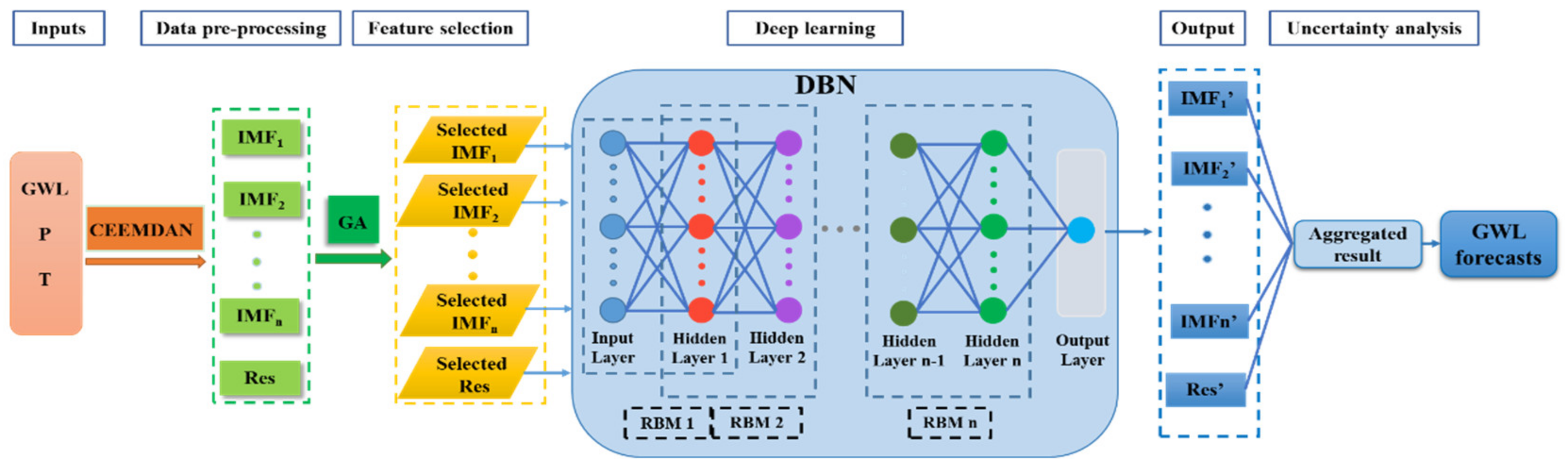
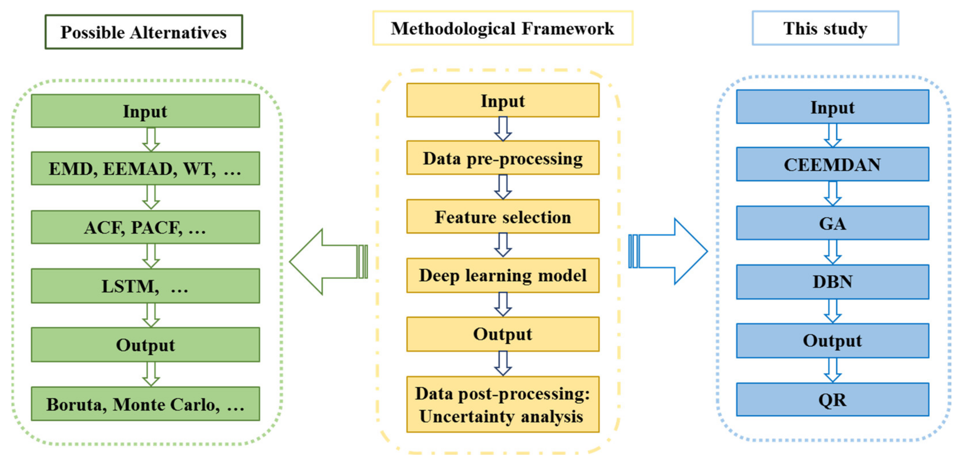
Considering the numerous machine learning applications in GWL forecasting, this study aims to implement an innovative and systematic hybrid modelling framework in GWL forecasting based on the integrated inclusion of data decomposition (data pre-processing), deep learning, feature selection and uncertainty evaluation (data post-processing) (
Table 1). The objectives are threefold.
(1) To develop a hybrid model (denoted as CEEMDAN-GA-DBN) with the highest configuration in data decomposition (CEEMDAN), feature selection (GA) and deep learning (DBN) and to test its validity in GWL forecasting at multi spatial and temporal scales for the arid Jiuquan Basin.
(2) To evaluate the robustness of the newly proposed GWL prediction scheme (i.e., CEEMDAN-GA-DBN) versus a pre-decomposed deep learning (i.e., CEEMDAN-DBN) model and a standalone deep learning (i.e., DBN) model.
(3) To evaluate all the possible uncertainties of the GWL forecasts by adopting the quantile regression (QR) method and combining the modelling procedure with the deterministic prediction results of the hybrid CEEMDAN-GA-DBN, the hybrid CEEMDAN-DBN and the standalone DBN model.
3. Results and Discussion
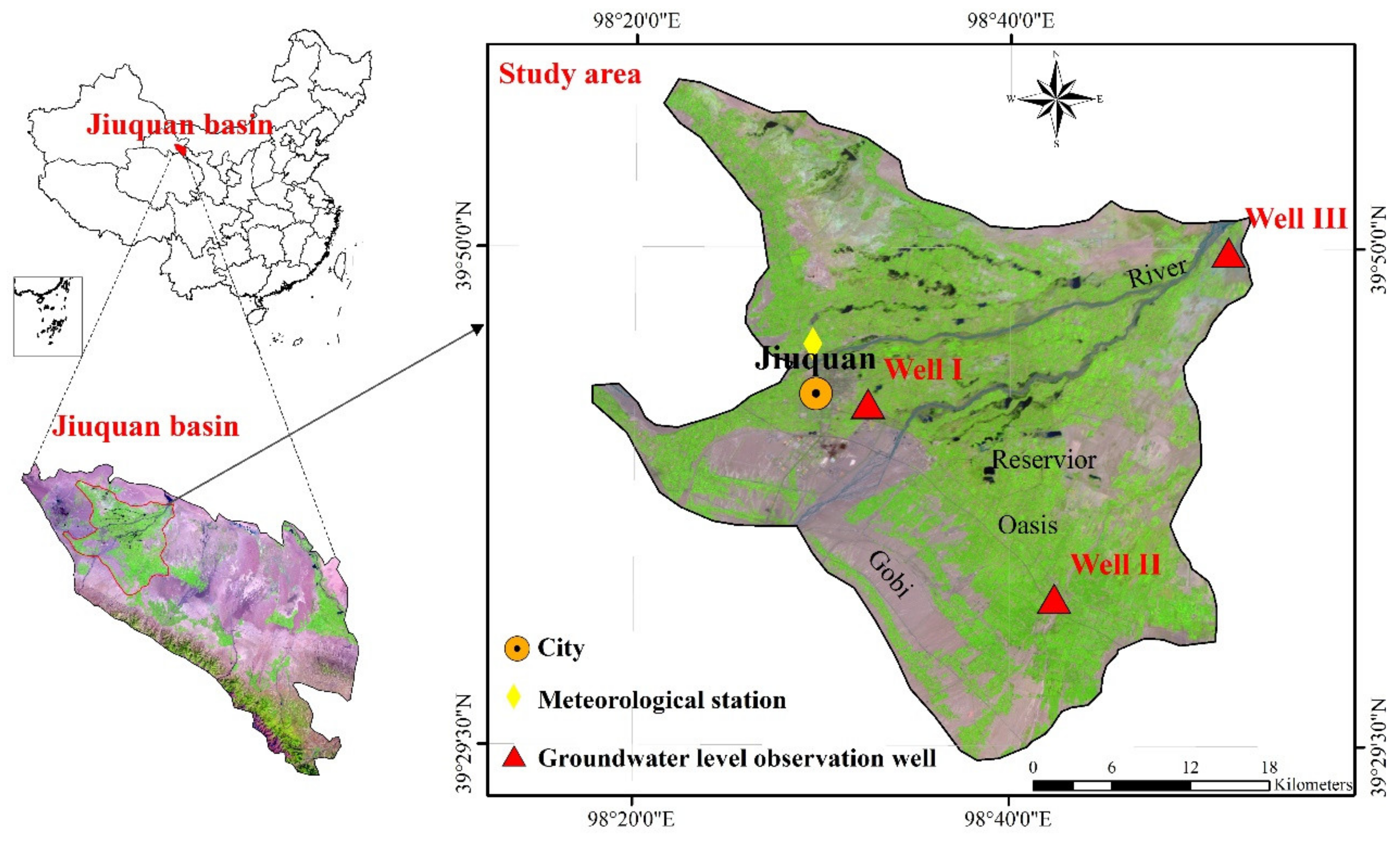
In this section, a comprehensive evaluation among the objective model (i.e., CEEMDAN-GA-DBN), the hybrid CEEMDAN-DBN and the standalone DBN models for 1-, 2- and 3-month ahead GWL forecasting is analyzed and discussed. The performance metrics of the CEEMDAN-GA-DBN, the CEEMDAN-DBN and the DBN models of Wells I, II and III (
Figure 2) in the training and the testing periods are enumerated in
Table 3,
Table 4 and
Table 5. Considering the GWL forecasting purpose in this study, the performance of the proposed models in the testing period is mainly focused.
3.1. Performance of the Hybrid CEEMDAN-GA-DBN Model
For 1-month ahead GWL forecasting, the hybrid CEEMDAN-GA-DBN model obtained very good performances at Well I, Well II and a good performance at Well III following the NSE and RSR values. Evidently, the hybrid CEEMDAN-GA-DBN model attained the R, MAE, RMSE, NSE and RSR values of 0.930, 0.210 m, 0.277 m, 0.819 and 0.421 for Well I, respectively, and 0.968, 0.254 m, 0.291 m, 0.929 and 0.264 for Well II, respectively. For Well III, the R, MAE, RMSE, NSE and RSR values were found to be 0.843, 0.110 m, 0.157 m, 0.688 and 0.554. Interestingly, the R values for all the three GWL observation wells were significantly higher than 0.80 for the 1-month ahead forecasting, while RMSE and MAE were relatively small. That is to say, the hybrid CEEMDAN-GA-DBN model developed in the present study was able to provide very accurate and reliable forecasts for 1-month ahead GWL forecasting.
For the prediction of the 2- and 3-month ahead, the evaluation metrics in the testing phase revealed that the performance of the hybrid CEEMDAN-GA-DBN model was worse at the 1-month ahead timescale. Hence, there was a notable reduction in the magnitudes of R and NSE, and a consequent increase in the magnitudes of errors (i.e., RSR, MAE and RMSE) for Well I, Well II and Well III. The result, demonstrating an inferior performance of the proposed model at the 2- and 3-month ahead timescales, was consistent with other studies [
38,
39]. However, the magnitude of the performance metrics remained within a high predictive accuracy range. Specifically, taking Well I for example, the hybrid model (CEEMDAN-GA-DBN) registered a value at the 2-month ahead forecast of R, MAE, RMSE, NSE and RSR equivalent to 0.904, 0.225 m, 0.315 m, 0.759 and 0.486, respectively, and the acquired values were 0.865, 0.247 m, 0.333 m, 0.735 and 0.513 for the 3-month ahead GWL forecast, respectively. Importantly, the prediction results showed that the hybrid CEEMDAN-GA-DBN model obtained relatively good performance for the 2-month ahead GWL prediction and acceptable results for the 3-month ahead GWL prediction for the case of Well I. Meanwhile, the present study also found that the R values in the testing period were greater than 0.90, the MAE and RMSE remained significantly low, the NSE values exceeded 0.80 and the RSR values were less than 0.50 for the case of Well II. For the case of Well III, the simulation results showed that the hybrid CEEMDAN-GA-DBN method obtained acceptable performance for 2- and 3-month ahead GWL prediction with the NSE values being greater than 0.50 and the RSR values being less than 0.70.
Despite the slightly deteriorated performance at the longer lead time, the R values in the testing period were greater than 0.75 for all the wells. The results stated clearly that the predicted GWL values fitted the target data quite closely. Indeed, the low MAE and RMSE values and the high NSE and RSR values demonstrated the high-quality forecast. It should be noted that the performance of the hybrid CEEMDAN-GA-DBN model was in agreement with that of the previous researchers who utilized machine learning models to predict the hydrological systems at multiple timescales [
71,
73]. In those studies, the predictive capacity of their models also deteriorated with an increase in the forecasting timescale, which may be attributed to the reduction in data patterns at longer time steps [
74]. Despite the deteriorated accuracy of 2- and 3- month ahead forecasting, statistical metrics for the hybrid CEEMDAN-GA-DBN model in the testing phase satisfied the requirements of good GWL simulation. Therefore, it is certain that the hybrid CEEMDAN-GA-DBN model achieved good forecasts for long-term GWL simulation.
3.2. Comparison of the CEEMDAN-GA-DBN Model, the CEEMDAN-DBN Model and the DBN Model
When comparing the capability of the hybrid CEEMDAN-GA-DBN, the CEEMDAN-DBN and the DBN models for 1-, 2- and 3- month ahead GWL forecasting, it can be seen that the proposed CEEMDAN-GA-DBN model outperformed the hybrid CEEMDAN-DBN and DBN models not only for the 1-month ahead GWL predicting, but also for the 2- and 3- month forecasting horizons (see
Table 3,
Table 4 and
Table 5).
Taking Well I for instance, for 1-month ahead forecasting, the hybrid CEEMDAN-DBN and the standalone DBN model yielded R, MAE, RMSE, NSE and RSR values of 0.923, 0.214 m, 0.313 m, 0.770, 0.476 and 0.881, 0.259 m, 0.341 m, 0.727, 0.518, respectively. By contrast, the hybrid CEEMDAN-GA-DBN model attained R and NSE values of 0.930 and 0.819, while the MAE, RMSE and RSR were reduced to 0.210 m, 0.277 m and 0.421, respectively. The CEEMDAN-GA-DBN model reduced 11.50% of RMSE less than the CEEMDAN-DBN model, and 18.77% less than the DBN model; while it improved NSE by 6.36% more than the CEEMDAN-DBN model, and 12.65% more than the DBN model. That is, the hybrid CEEMDAN-GA-DBN predictive model developed in this study provided more accurate and reliable 1-month ahead GWL forecasting compared with the CEEMDAN-DBN and DBN models (see
Table 3,
Table 4 and
Table 5). Although the accuracy of the 2- and 3-month ahead predicted GWL values was worse than that of the 1-month forecasts, the present results obtained using the hybrid CEEMDAN-GA-DBN model were comparatively better than the other two models. For example, compared with that of the CEEMDAN-DBN (0.363 m) and DBN (0.396 m) models, the RMSE of the CEEMDAN-GA-DBN decreased by 8.26 and 15.91%, respectively, for 3-month ahead forecasting. Overall, the CEEMDAN-GA-DBN reduced the RMSE of the CEEMDAN-DBN and DBN models in the testing period about 9.16 and 17.63%, while it improved their NSE by about 6.38 and 15.32%, respectively, for all the lead times and the three wells.
The hybrid CEEMDAN-GA-DBN model can also be considered good since the NSE value was 0.840 and the RSR value was 0.397 for the 2-month ahead forecasting at Well II. In contrast, the hybrid CEEMDAN-DBN and DBN models were inferior to the CEEMDAN-GA-DBN. The NSE values reduced to 0.789 and 0.730, while the RSR values increased to 0.456 and 0.515 for the 2-month ahead forecasting of Well II. The results demonstrated the better performance that the hybrid CEEMDAN-GA-DBN model achieved. Similarly, the hybrid CEEMDAN-GA-DBN model yielded more accurate results than the hybrid CEEMDAN-DBN and DBN model for the 3 month-ahead GWL simulation. Therefore, the simulation results reveal that the hybrid CEEMDAN-GA-DBN method can significantly improve performance relative to the hybrid CEEMDAN-DBN and the standalone DBN model in terms of the 2- and 3-month ahead GWL estimations.
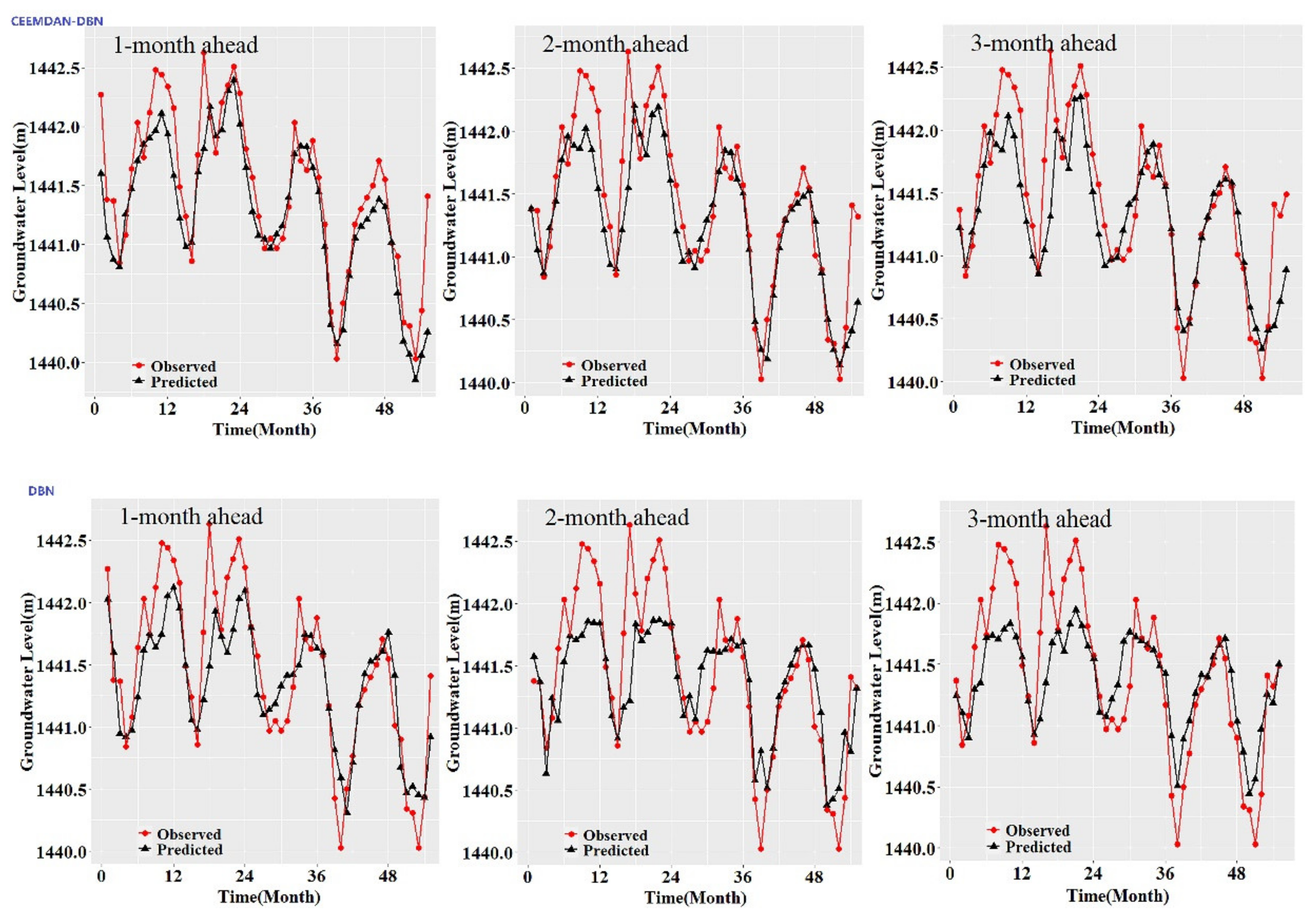
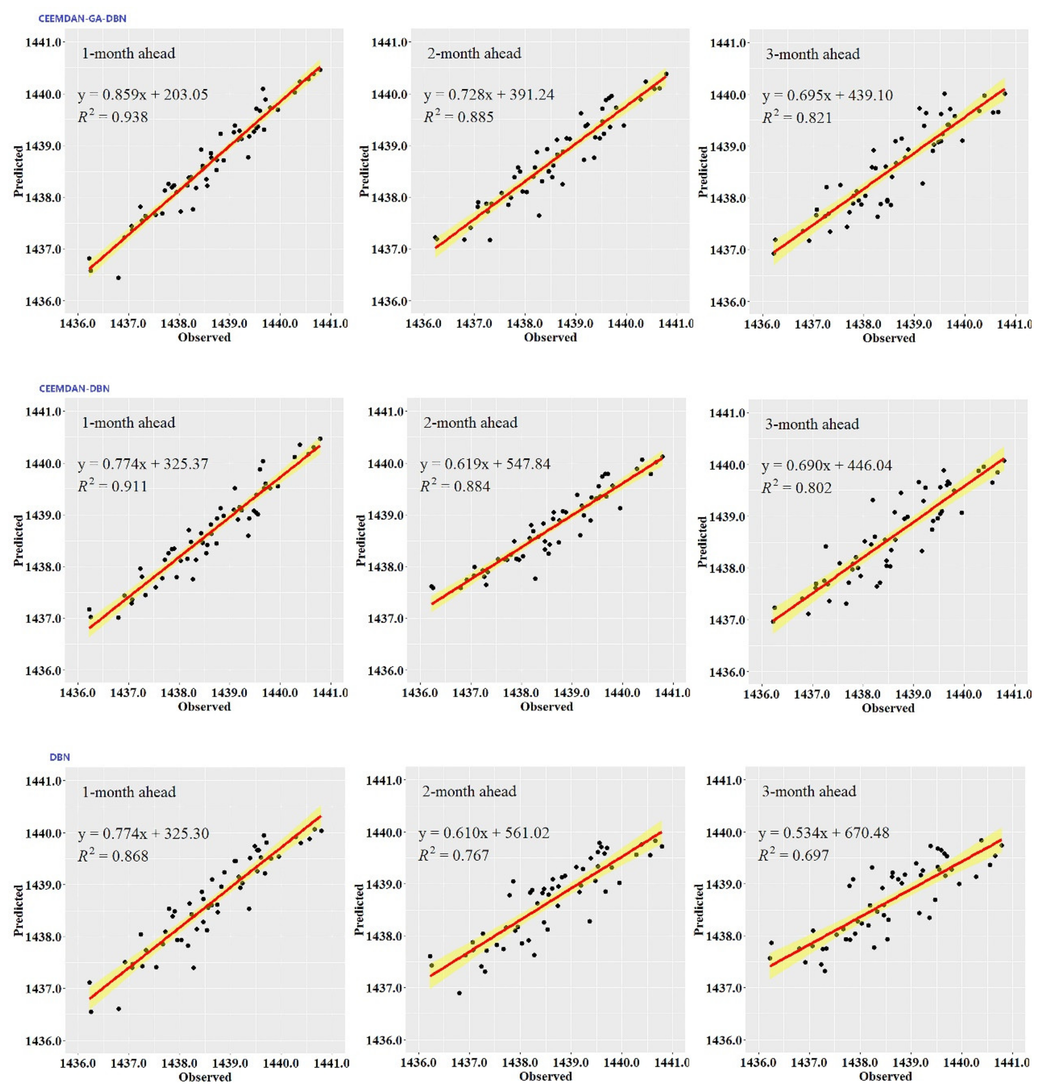
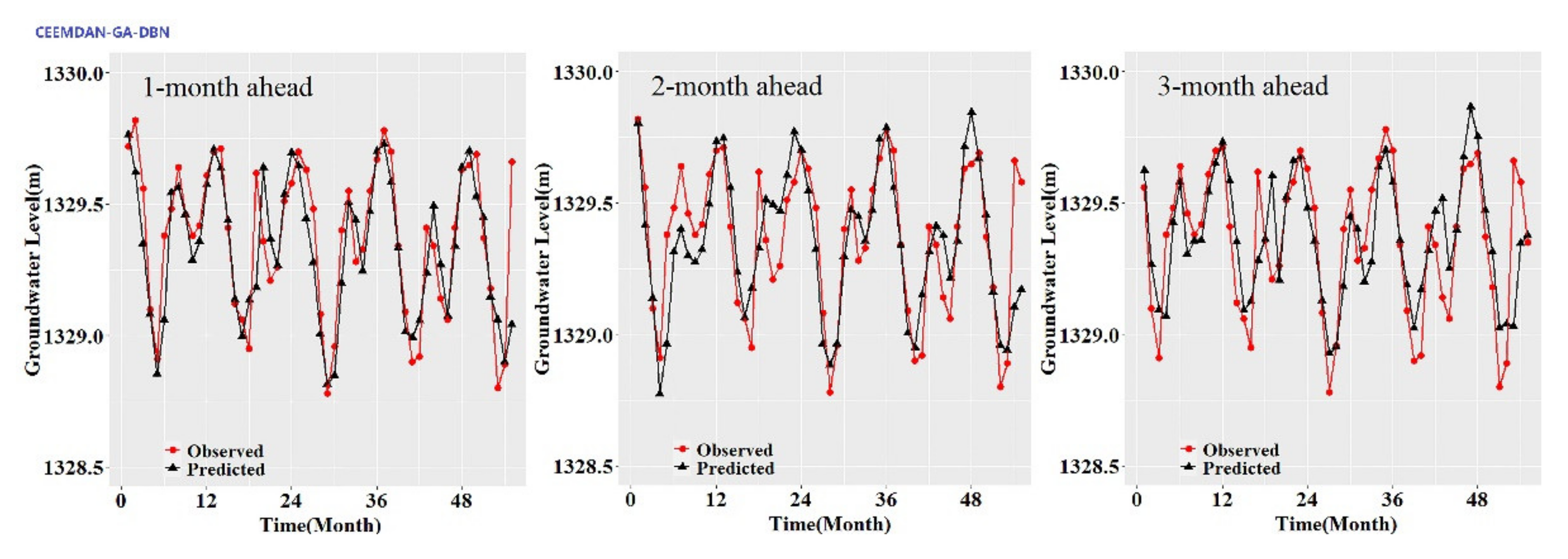
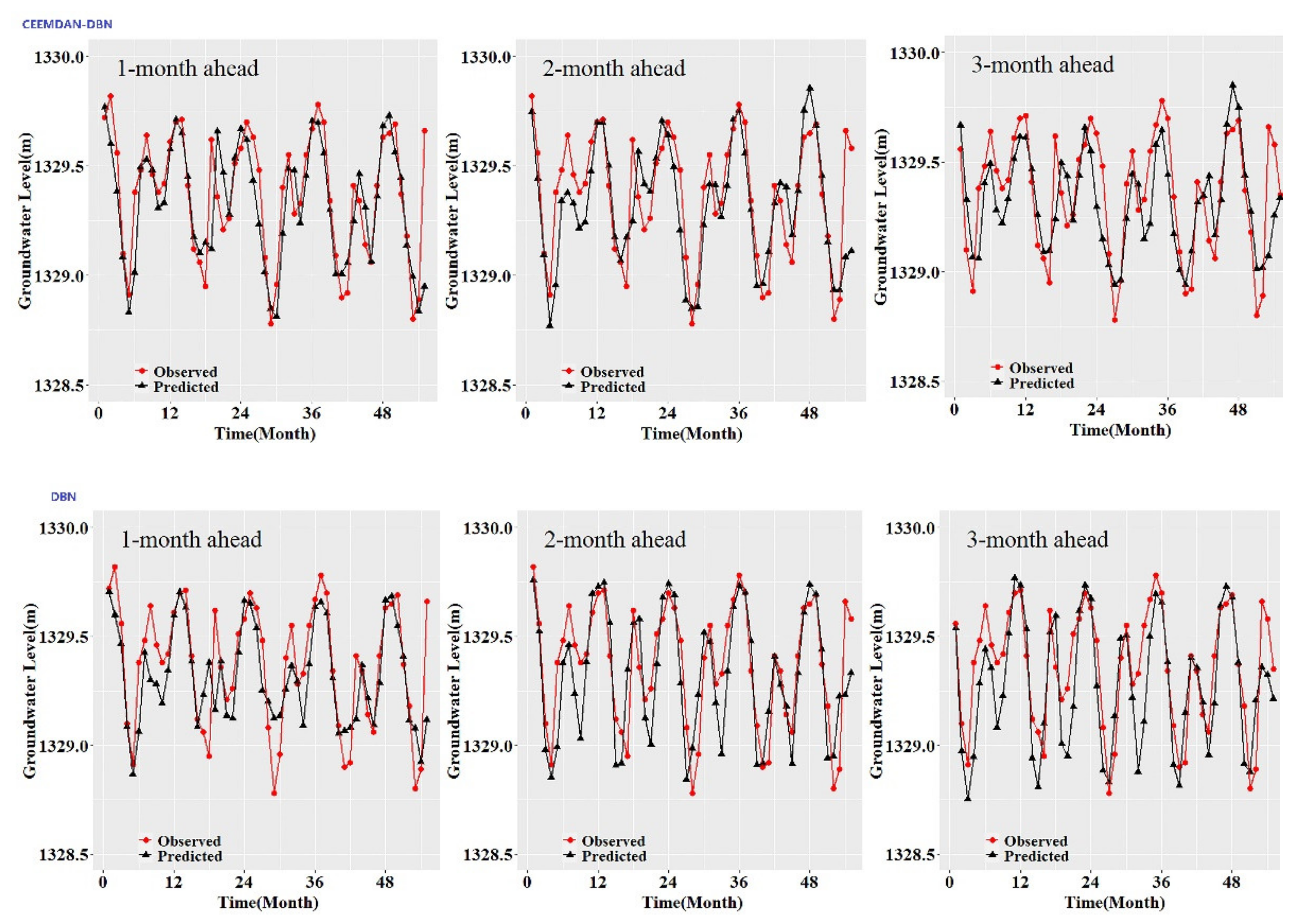
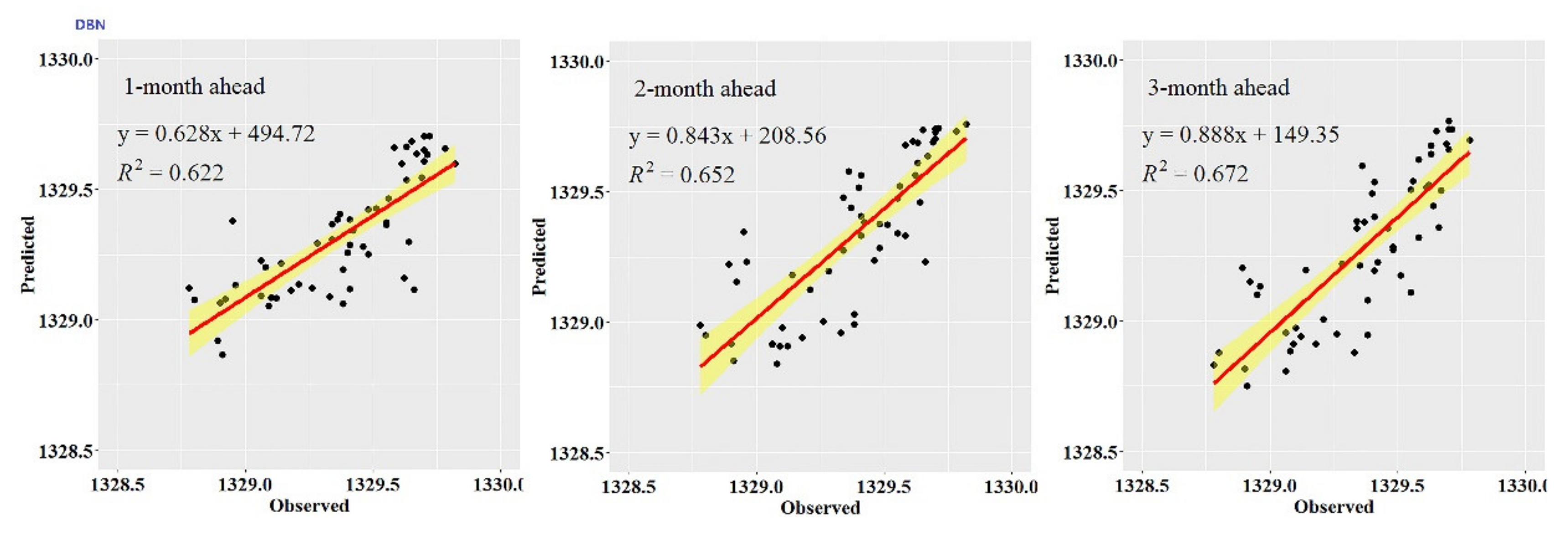
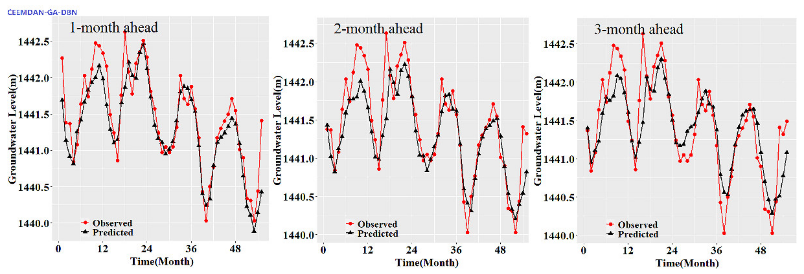
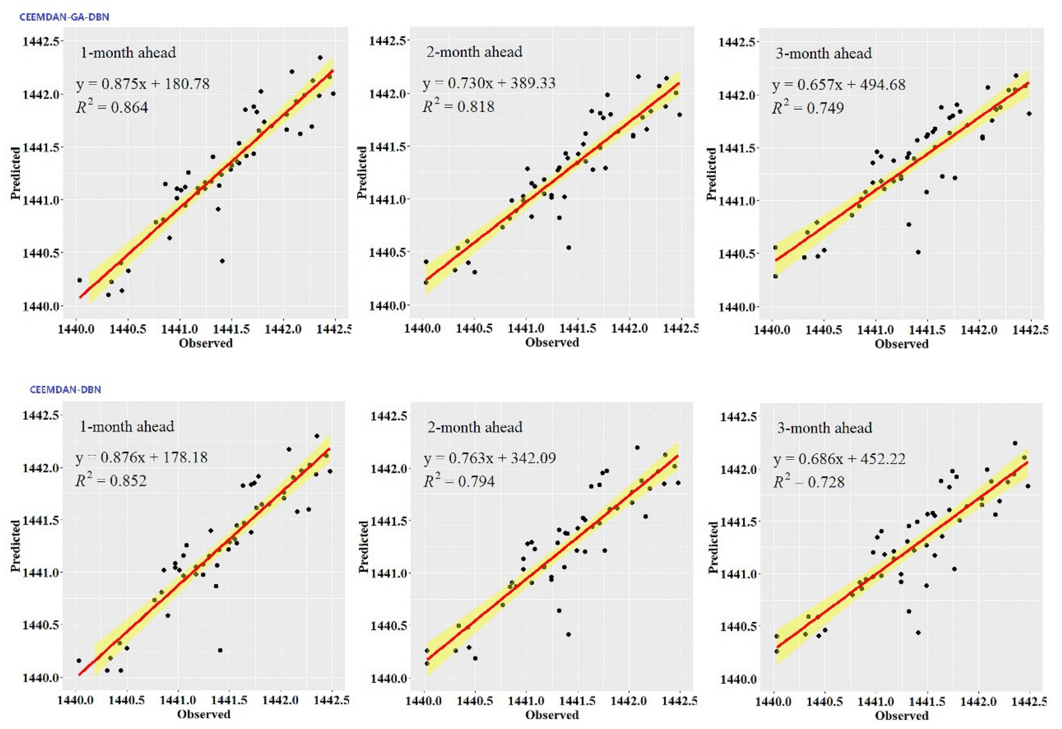
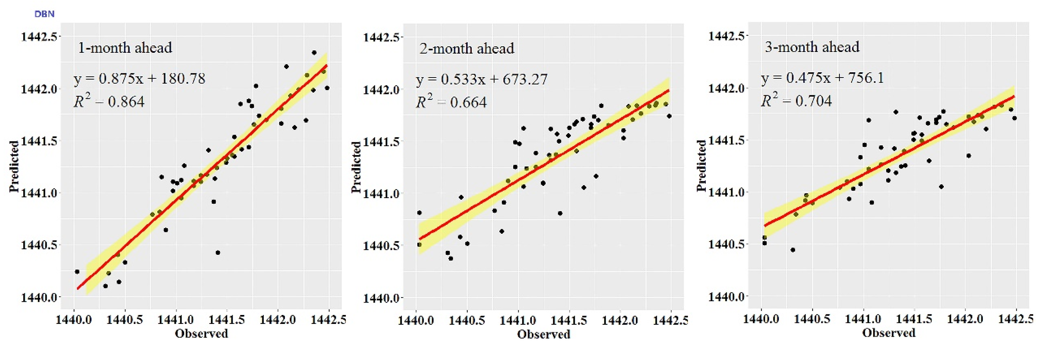
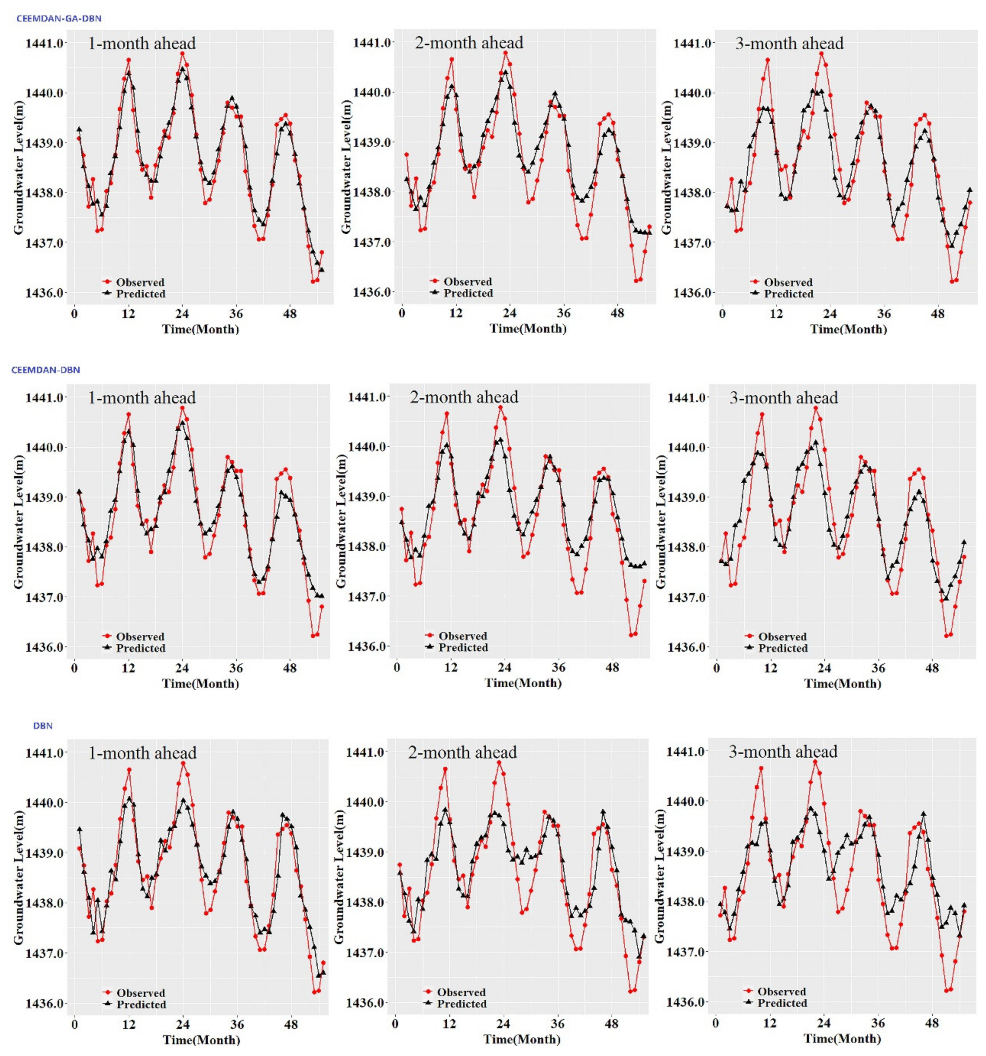
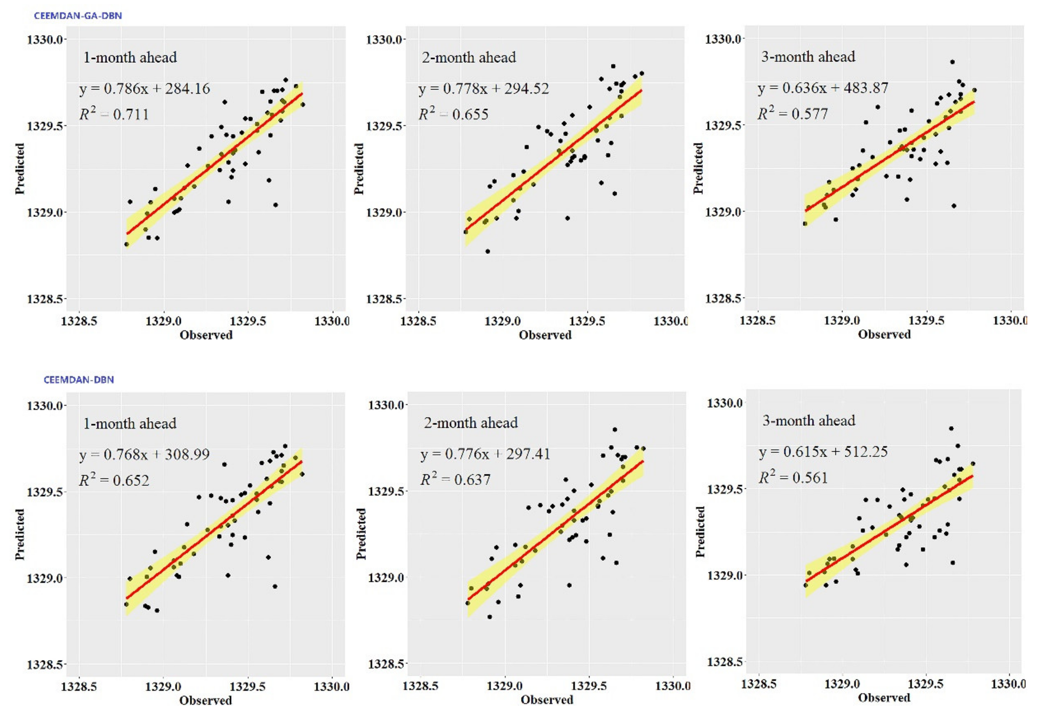
While the performance metrics can statistically evaluate the ability of the CEEMDAN-GA-DBN, the CEEMDAN-DBN and the DBN models, the hydrograph and scatter plots are capable of assessing and displaying the temporal correspondence of the observed GWL data and the predicted values.
Figure 3,
Figure 4,
Figure 5,
Figure 6,
Figure 7 and
Figure 8 show the hydrographs and scatter plots of the observed and predicted GWL at the 1-, 2- and 3-month ahead times for the CEEMDAN-GA-DBN, CEEMDAN-DBN and DBN models in the testing period. For interpretation purposes, the least square regression line, y = ax + b was incorporated in each panel. The constant a and intercept b were used to assess the model’s overall accuracy. Clearly, the CEEMDAN-GA-DBN model performed far better for 1-month lead GWL forecasting than the 2- and 3-month lead time. The performance for a longer lead time deteriorated gradually (
Figure 3,
Figure 4,
Figure 5,
Figure 6,
Figure 7 and
Figure 8). Furthermore, it is apparent that the GWL forecasted using the CEEMDAN-GA-DBN model closely matched with the corresponding observed values.
Figure 3,
Figure 4,
Figure 5,
Figure 6,
Figure 7 and
Figure 8 also show the hydrographs and scatter plots of the observed and estimated GWL values generated using the CEEMDAN-DBN and DBN models in the testing period. Both the CEEMDAN-DBN and DBN models show relatively good accuracy for the 1-, 2- and 3-month ahead GWL forecasting. Moreover, it can be seen from the fitted equations that the CEEMDAN-GA-DBN model yielded a and b closer to 1 and 0 when compared with that of the CEEMDAN-DBN and DBN models in most cases. The results demonstrated the significantly better fit the CEEMDAN-GA-DBN model achieved. These figures confirmed that the CEEMDAN-GA-DBN model has a better generalization skill of the predictive data compared with the CEEMDAN-DBN and DBN models considered in the current study. Thus, the best accuracy in GWL forecasting was achieved using the CEEMDAN-GA-DBN model.
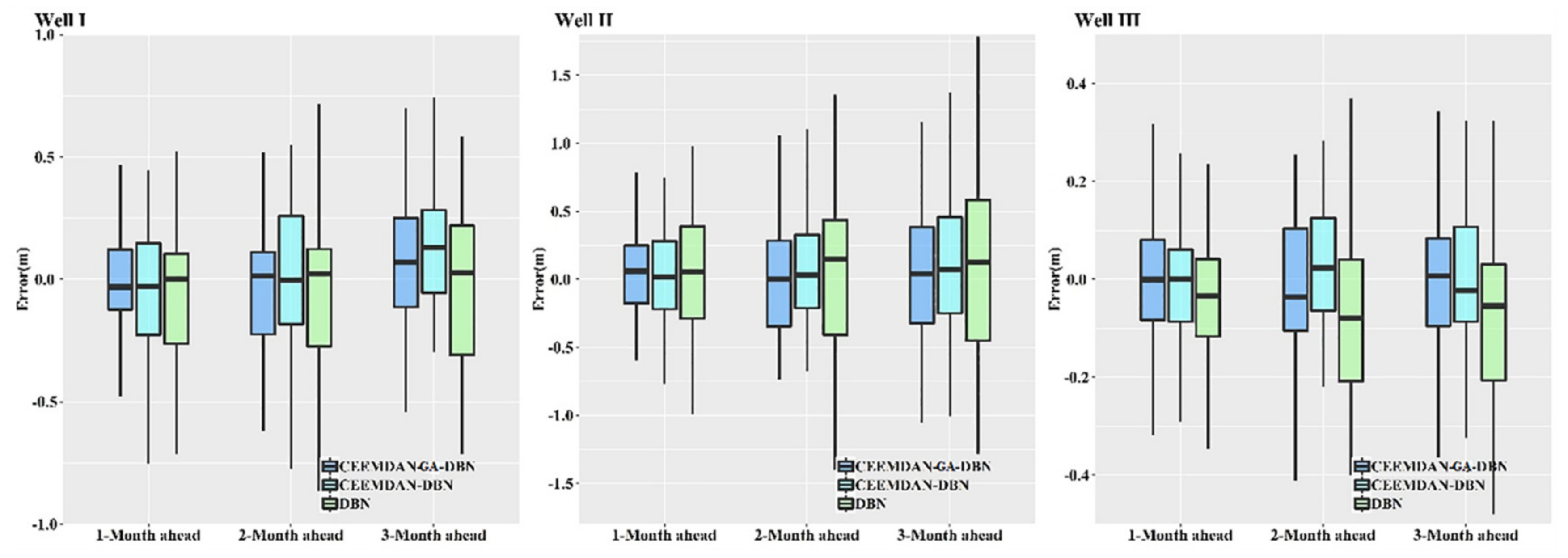
When evaluating the feasibility of a predictive model in GWL prediction, the distribution of error can show a robust and reliable consequence of the model’s predictability.
Figure 9 demonstrates the error indicators for the hybrid CEEMDAN-GA-DBN, CEEMDAN-DBN and DBN models. The boxplot diagram shows the degree of the dispersion and skewness of the error for all the wells. Clearly, the figure illustrates that the CEEMDAN-GA-DBN technique obtained the minimum error compared with the CEEMDAN-DBN and DBN models in most instances. This is especially true for the 1-month ahead GWL prediction and the 2- and 3-month ahead prediction values. Therefore, the current results confirm that the CEEMDAN-GA-DBN model is superior to the CEEMDAN-DBN and DBN models in terms of error distributions.
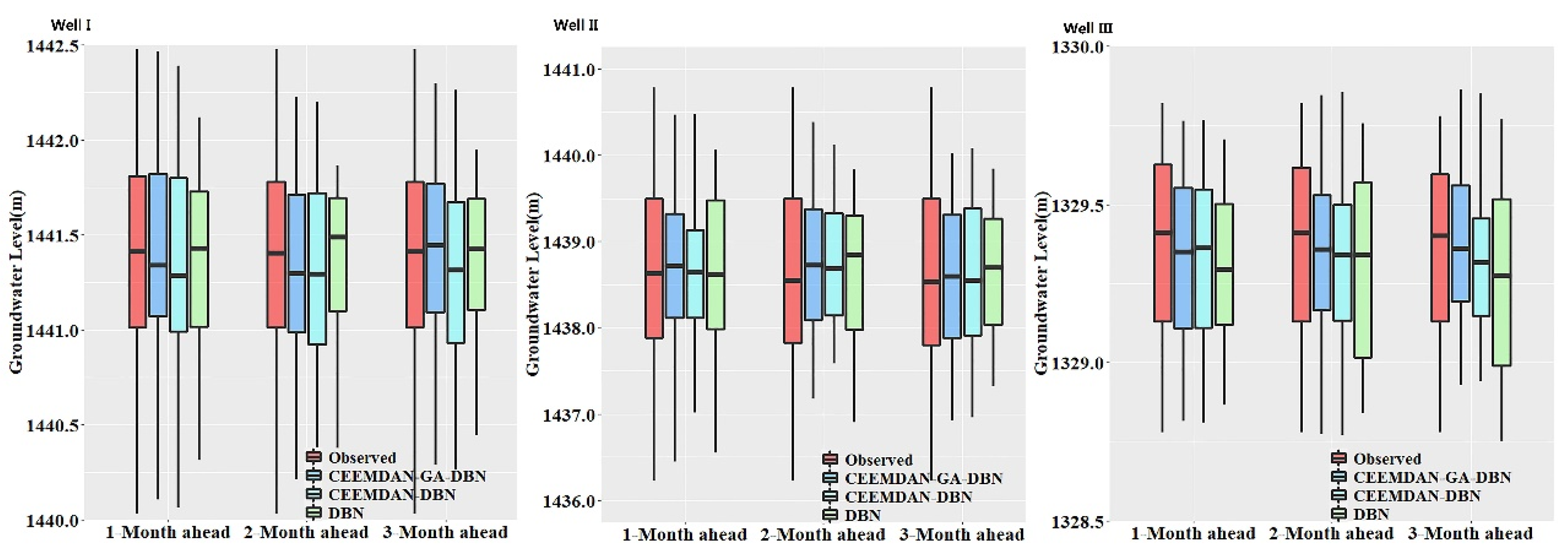
A visualized comparison of the distribution of the observed and forecasted values for a forecasting model is an effective way to verify and validate a model. Considering that the boxplot can present a clear visualization of the data distribution concerning the quartiles distinctly indicating the outliers. The boxplots diagrammatizing the distribution of the observed and forecasted GWL values from the CEEMDAN-GA-DBN, CEEMDAN-DBN and DBN models are shown in
Figure 10. It can be seen that the box areas for all three models are very close to the observed values. Comparatively speaking, the distribution of the CEEMDAN-GA-DBN-forecasted GWL approaches the observed GWL values than the CEEMDAN-DBN and DBN models under most circumstances. Consequently, it is further ascertained that the CEEMDAN-GA-DBN model is expected to generate forecasted GWL values that closely resemble the measured values.
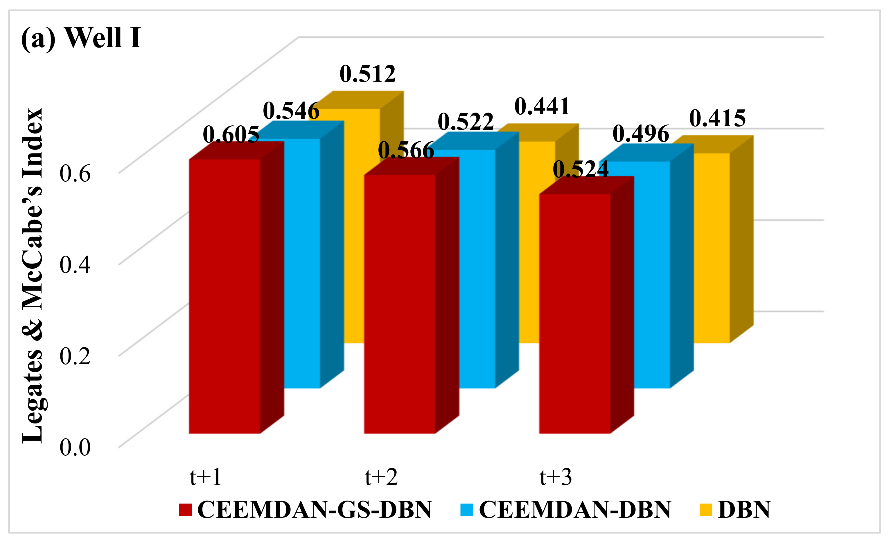
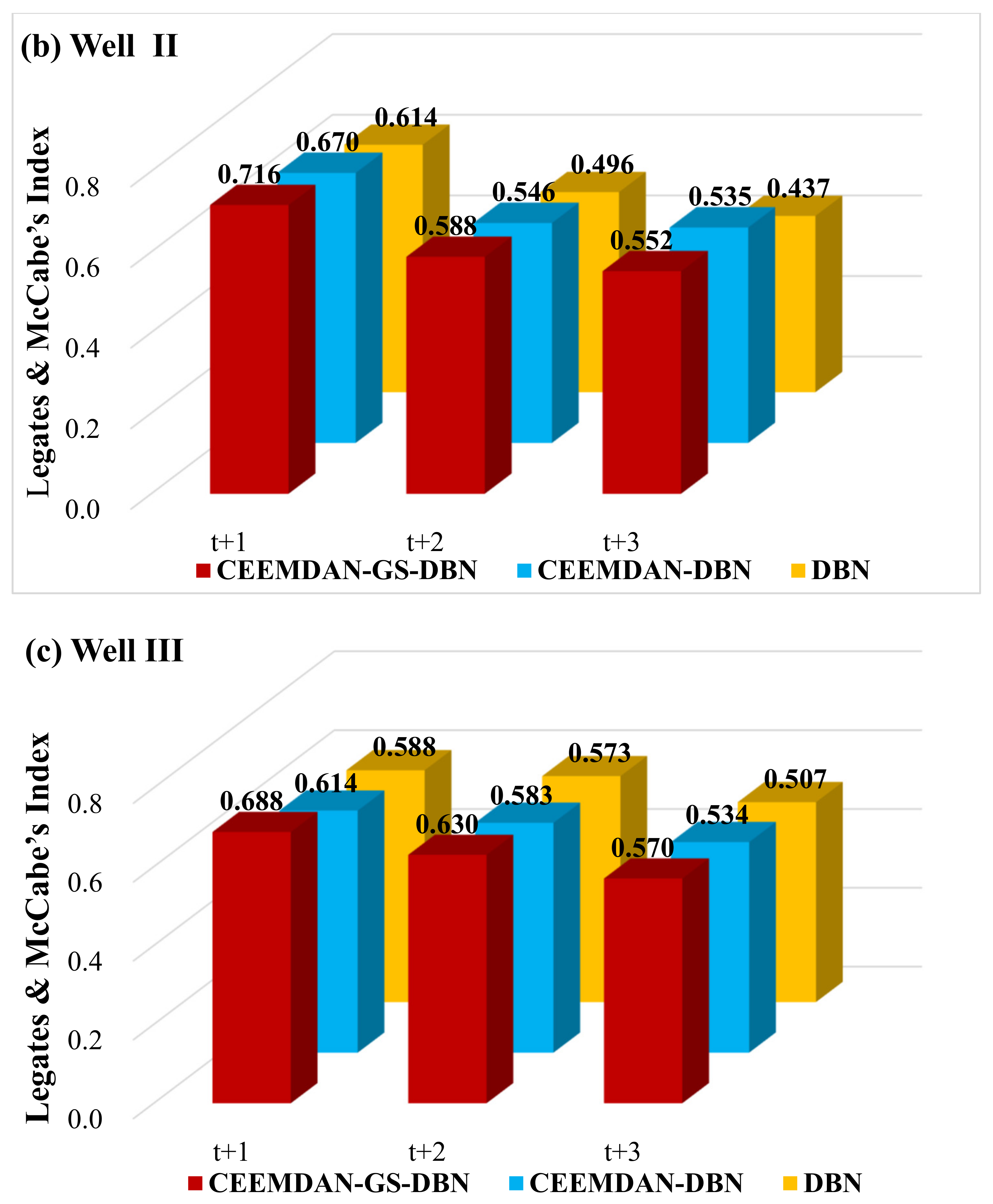
To determine the accuracy of the hybrid CEEMDAN-GA-DBN model, the Legates and McCabe’s Index was imported.
Figure 11 plots the Legates and McCabe’s Index computed for all the simulated and observed GWLs in the testing phase. It is noteworthy that for a perfect model, the index must approach one. There is no doubt that the hybrid deep learning model (i.e., CEEMDAN-GA-DBN) produces significantly better forecasts, evidenced by the larger Legates and McCabe’s Index. This is important for all the forecasting horizons, ranging from t + 1 to t + 3, although the accuracy deteriorates as the forecast horizon increases. Nonetheless, the performance of the CEEMDAN-GA-DBN model, where the data decomposition was used together with the feature selection, far exceeds that of the CEEMDAN-DBN and the standalone DBN model.
In terms of model simplicity, the AIC index was used to compare the performance of the proposed methods.
Table 6 shows the AIC values of the CEEMDAN-GA-DBN, CEEMDAN-DBN, DBN models for 1-, 2- and 3-month ahead GWL forecasting at three GWL wells. It can be clearly seen that the CEEMDAN-GA-DBN obtained the lowest AIC values, while the DBN model derived the highest AICs. Taking the results of Well I as an example, the DBN model obtained AIC values of −114.275, −98.281 and −97.732, respectively at three forecasting horizons; however, the AIC values of the CEEMDAN-DBN model decreased by 8.12, 18.93 and 9.62%; for the CEEMDAN-GA-DBN model, the AIC values reduced by 19.81, 24.88 and 19.50%. The results indicate that the data decomposition and feature selection processes improved the accuracy of the model rather than increasing model complexity. Therefore, combining the above accuracy and complexity analysis results of the proposed models, it can be found that although the CEEMDAN-GA-DBN model had two more steps (data decomposition and feature selection) than the other models, it is able to achieve a simpler and more accurate model.
3.3. Uncertainty Analysis
Typically, higher GWL prediction accuracy means less uncertainty and smoother fluctuations, which is significant for the utilization and planning of groundwater resources. Therefore, analyzing the uncertainty of the proposed models in GWL simulation is of great significance. In this study, the predictive uncertainties of the CEEMDAN-GA-DBN, CEEMDAN-DBN and DBN models were assessed using the QR, the uncertainty information of GWL predictions was estimated at 90 and 95% confidence levels.
Table 7 and
Table 8 present the MPI and PICP values of different wells and different forecasting horizons. Note that perfect reliability is shown as the PICP value equals the corresponding confidence level. If similar PICP scores are derived, then the one with lower MPI is the better. The tables show that the uncertainty analysis results of the CEEMDAN-GA-DBN, CEEMDAN-DBN and DBN models are not identical in terms of the MPI and PICP values either at the confidence level of 90% or the confidence level of 95%. It seems very difficult to derive balanced low MPI as well as high PICP values since other researchers also encountered this problem [
65,
66]. Nevertheless, the PICP values of the proposed CEEMDAN-GA-DBN model are higher than that of the CEEMDAN-DBN and DBN models in most circumstances. Although higher PICP values can be found in the CEEMDAN-DBN and DBN models in some conditions, their MPI values remain higher than the CEEMDAN-GA-DBN model. Hence, the proposed CEEMDAN-GA-DBN method exhibits a slightly better forecasting reliability compared with the CEEMDAN-DBN and DBN models on the whole.
3.4. Model Interpretation
From the viewpoint of the predictive performances and uncertainty criterion, it can be appropriately concluded that the proposed CEEMDAN-GA-DBN model provides a more robust and stable predictive performance in GWL forecasting for multiple forecasting horizons. The high precision of the hybrid CEEMDAN-GA-DBN model may lie in three aspects. Firstly, the deep belief network algorithm can discover the inherent physical structure and antecedent features powerfully in datasets without prior knowledge. Therefore, the high-level nonlinear groundwater dynamic characteristics can be effectively captured through a deep learning process. Secondly, the intrinsic mode functions (IMFs) decomposed by the CEEMDAN algorithm express the non-stationary and uncertainty behaviors of GWL more clearly, making the repeating feature catching process more reliable and predictable. That is the reason for the much better prediction performance of the CEEMDAN-DBN model than the DBN model. Thirdly, the irrelevant and redundant attributes of the GWL were identified and removed from the IMFs using the genetic algorithm-based feature selection procedure, thus the accuracy and stability of the model was improved. However, the inconformity of the uncertainty analysis results among the three wells and the three models reveals that uncertainty is inevitable, even for those models with high accuracy. Typically, the uncertainty increases as the noise increases [
65]. In this study, reasonable interpretations for this phenomenon may lie in the collective affect from every possible step of the methodological framework, the hydrogeological heterogeneity of the three distinguished GWL observation wells, the observed GWL data (the observation or the data entry processes) and the other sources.
However, when comparing the performance of the proposed models in training and testing phases, it can be seen that the performance in the former phase is much better than that in the testing phase in most cases, meaning there is a phenomenon of overfitting to some extent. Overfitting is an issue within machine learning based applications where a model learns the patterns of the training dataset too well, perfectly explaining the training set but failing to generalize this predictive power to other sets. Actually, in this study, the cross-validation procedure was applied to deal with this problem through dividing all the data into two distinct sets: the training set and the testing set, but still did not avoid it. Through a comprehensive literature review, it can be found that the phenomenon that the performance in the training period is superior to that in the testing period is common in machine learning/deep learning based GWL forecasting studies [
75,
76]. In this study, according to the derived results, although the MAE values in the testing phase were higher than that in the training phase, the MAE for Well I, Well II and Well III was less than 0.4, 0.7 and 0.2 m, respectively. Compared with the average GWL of 1141.36, 1138.73 and 1329.33 m of the three GWL wells, the error is acceptable. Moreover, the analysis in this study also proved that the proposed model achieved high accuracy since the magnitude of the other performance metrics remained within high predictive accuracy ranges in both the training and testing periods. Considering this, it can be said that the overfitting problem only demonstrates the inferior generalization ability of the proposed models, rather than the accuracy or the application of the model.
In addition, it is noteworthy that in the irrigated areas of the Jiuquan basin (e.g., this study area), the dynamics of the phreatic groundwater are closely related to agricultural irrigation. The irrigation water infiltration has important significance to the replenishment of the groundwater in this area. That is mainly because the groundwater level drops when pumping during irrigation time, while it rises after irrigation. Overall, the variation of the GWL changes little over the years, thus no obvious upward or downward trend was found [
77]. This means that the proposed model and derived results in this study remain useful in multi time steps ahead GWL forecasting since the GWL dynamics were captured using the CEEMDAN-GA-DBN model through the training process.
4. Conclusions
The accurate and reliable GWL prediction is extremely important for the planning and management of groundwater resources in arid irrigated regions. In this study, a novel hybrid forecasting framework (the CEEMDAN-GA-DBN model) was proposed for 1-, 2- and 3-month ahead GWL prediction. The performance of the CEEMDAN-GA-DBN model was compared with the hybrid CEEMDAN-DBN model and the standalone DBN model by the performance metrics and uncertainty criterion.
The results show that the hybrid CEEMDAN-GA-DBN model is able to successfully forecast 1-, 2- and 3-month ahead GWL and outperform the CEEMDAN-DBN and DBN model in terms of the performance criteria including R, MAE, RMSE, NSE, RSR and the Legates and McCabe’s Index. Moreover, based on the QR method, the proposed CEEMDAN-GA-DBN model is also very effective from uncertainties analysis. Therefore, it is certain that the CEEMDAN-GA-DBN model has a high potential for practical application in GWL prediction in arid irrigated areas. The CEEMDAN-GA-DBN model can be explored as a scientific tool applied for GWL forecast without understanding the intrinsic mechanisms and hydrogeological characteristics or collecting the condition data required for various interacting elements. Therefore, it is especially valuable for regions with limited measurement data to develop a physical based hydrogeological model. Yet, attention should be paid to the uncertainty in the process of model building.
The implementation of the CEEMDAN-GA-DBN proves the conspicuous results of the proposed framework, indicating a forecasting framework that, when implemented in practice in arid irrigated areas, can improve the GWL forecasting accuracy. Considering the extensive range of feature selection methods and deep learning models, in further studies, any other methods can be explored as alternative tools in their place if necessary (
Figure 12).
Although the proposed deep learning model has achieved an excellent accuracy for GWL prediction, considerable room remains for further improvement. Firstly, due to a lack of data in recent years, the performance of the model was mainly focused from 2000 to 2015. Considering the fact that in recent years, water demand has increased dramatically, and groundwater has been excessively exploited with an annual groundwater extraction rate of 2.6 × 10⁸ m3, whether the same high accuracy can be derived using the model remains uncertain and needs to be further studied. Secondly, a comprehensive assessment should be implemented to analyze the possible uncertainties that had influences on the performance of the models. For example, the spatial variation of the hydrogeological parameters should be considered in a future study to improve the model’s accuracy. Thirdly, certain anthropic or natural factors in the specific area, such as the excessive groundwater extraction, the change of water users as well as the irrigated areas in this groundwater-supported agricultural region, the intricate and intense interaction between river and groundwater in this inland river basin, may affect the accuracy of the GWL forecast. Therefore, there stands a chance that the model’s accuracy will be improved remarkably if these universal interfering factors and the controlling factors of different wells are taken into consideration. Finally, the performance of the CEEMDAN-GA-DBN model for 1-, 2- and 3-month ahead GWL forecasting was mainly discussed in this study; however, as a designed simulation model, further investigation of its potentiality in both short- and long-term forecasting would be an interesting exploration.


