First, a performance analysis of the OpenMP parallel code was conducted to decide the parallel granularity. Then, two open channel flows were simulated to test the accuracy of the model. Finally, two test cases of hydraulic jumps with different Froude numbers were considered, to validate the accuracy of the model in computing the hydraulic jumps.
3.1. Performance Analysis on Environment Variables
Load balancing is one of the key factors affecting the performance of OpenMP multithreaded programs. According to the execution principle of OpenMP, waiting between threads in a parallel program, which will inevitably lead to the inefficiency of the parallel program, will be significantly longer if the load imbalance in OpenMP program cannot be effectively controlled. Static, dynamic, guided, and runtime are four main scheduling strategies in OpenMP [
15]. Runtime scheduling was used to select one of the first three scheduling strategies based on the environment variable OMP_SCHEDULED in OpenMP. Therefore, runtime scheduling was not considered in the following calculations.
To the largest extent possible, all loop iterations were divided into blocks of the same size by Static scheduling. These iterations were divided equally if block size was not specified. n was assumed to be the total number of iterations. m was assumed to be the total number of threads in the parallel area. Subsequently, n/m iterations were assigned to every thread when the block size was the default. When the block size was set, successive iterations with the block size were assigned to each thread. Thus, the total workload was approximately divided into n/size blocks that were subsequently allocated to each thread in turn according to the rotation rule. An internal task queue was used by dynamic scheduling. A thread was allocated a certain number of iterations, specified by block size when it was available. When a thread completed its currently allocated block, the next block was taken from the head of the task queue. It should be noted that dynamic scheduling required additional overhead. Guided scheduling was similar to dynamic scheduling, to the extent that block size started large and subsequently decreased gradually. Therefore, guided scheduling was able to reduce the time to access queues for threads.
The parallel speed-up
Rs is compared in
Figure 3 for a hydraulic jump test case to test the efficiency of the parallel SPH code. In
Figure 3, the coordinate
x is the block size of the scheduling strategy. The coordinate
y is the parallel speed-up
Rs. The color of the line represents the scheduling strategy, where a red line is the result of a serial program. P
1–P
4 represent discrete particle numbers in the calculation domain. The parallel code runs on an Intel(R) Core (TM) i5 CPU with 2 cores, 4 threads, and a main frequency of 3.2 GHz. The total particle numbers are the sum of the boundary particles and the fluid particles at the initial time. These did not change much when the simulation became stable. The parallel speed-up was calculated as:
where
tp represents the execution time of the parallel code while
ts represents the execution time of the serial code.
In
Figure 3, the parallel speed-up of serial code is 1.0, based on the parallel speed-up equation. The execution time is the average time of ten runs. Default scheduling achieves no acceleration, while it makes the parallel execution time greater than the serial execution time. The reason for this may be that all boundary particles are distributed to one core by default, due to the sequential iteration of fluid particles and boundary particles in the loop. Subsequently, the waiting time of the core dealing with boundary particles is long because the running time of the fluid particles is longer than that of the boundary particles. Ultimately, the parallel execution time is longer than the serial time due to an unbalanced load. The speed-up of the guided scheduling is not obvious and is relatively stable. The speed-up essentially did not change with block size, except as shown in
Figure 3a. However, the speed-ups of static and dynamic scheduling re quite obvious. When particle numbers are less than 1 million, the parallel speed-up of static scheduling is higher than that of dynamic scheduling, while the opposite is true when particle numbers are greater than 1 million. All the maximum parallel speed-up of static scheduling was achieved at a block size of 10, except as shown in
Figure 3c. For dynamic scheduling, the block size of the maximum parallel speed-up increased gradually from 20 to 100, as particle numbers increased. Therefore, static scheduling was selected and block size was set to 10, while a smaller particle number was considered for the 2D hydraulic jumps. These particle numbers are usually less than 0.2 million. At this point, the parallel speed-up could reach about 2.0.
3.2. Open Channel Flow
Two uniform laminar flow test cases of open channels [
18] were simulated. The length of the numerical channel was 1.0 m. The slope was 0.04% for case 1 and 0.1% for case 2. The corresponding initial water depth
h0 was 0.1 m and 0.2 m, respectively. To obtain laminar flow, the dynamic viscosity
μ was set to 1.0
10
−1 N
s/m
2 for case 1 and 6.0
10
−1 N
s/m
2 for case 2, respectively. The Reynolds numbers
of the two test cases were 200 and 100. The channel bed was the non-slip boundary. A uniform velocity that was calculated using the formula in [
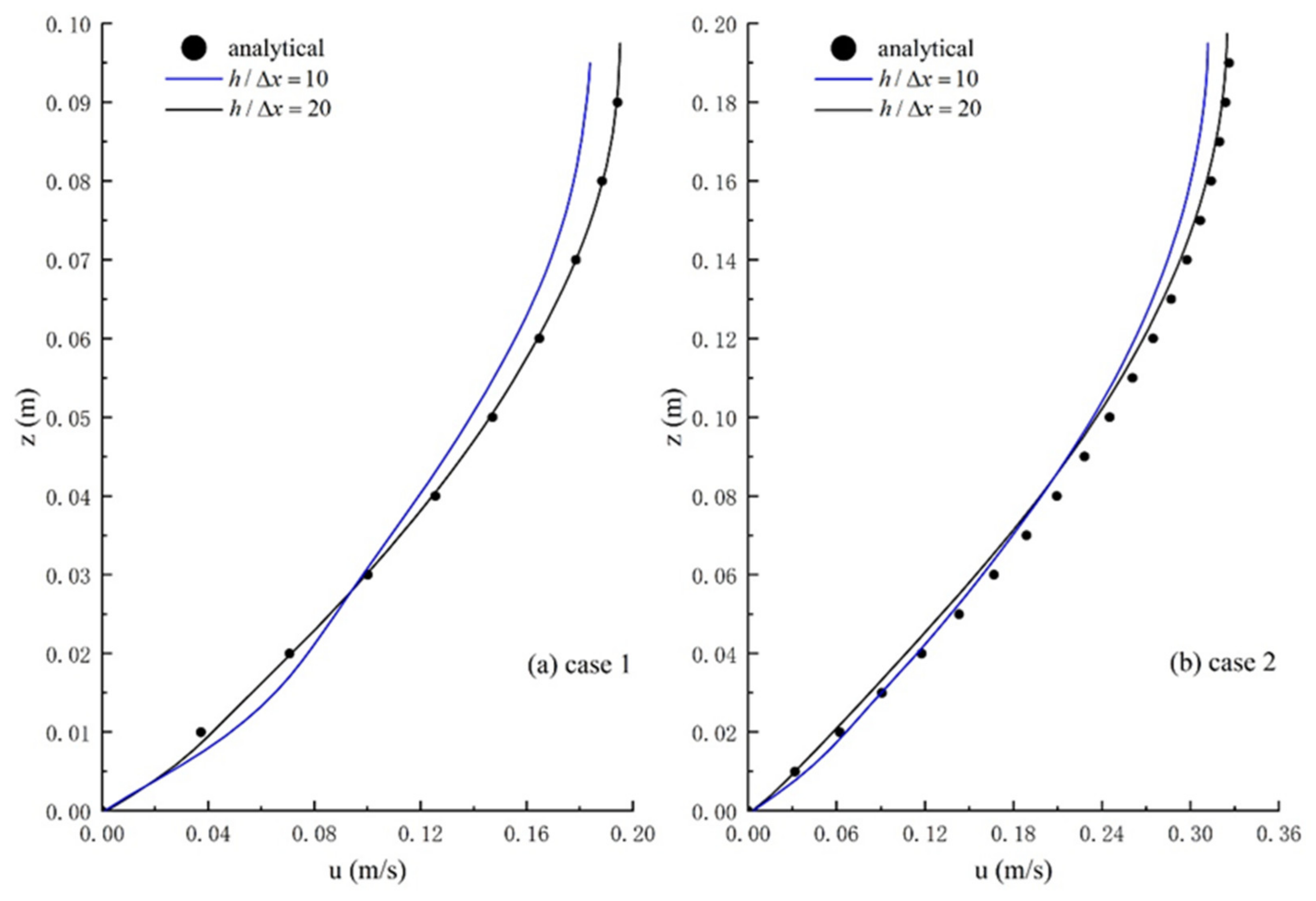
9] was given to the inlet particles. The outlet boundary was free outflow. To analyze the adequacy of the particles,
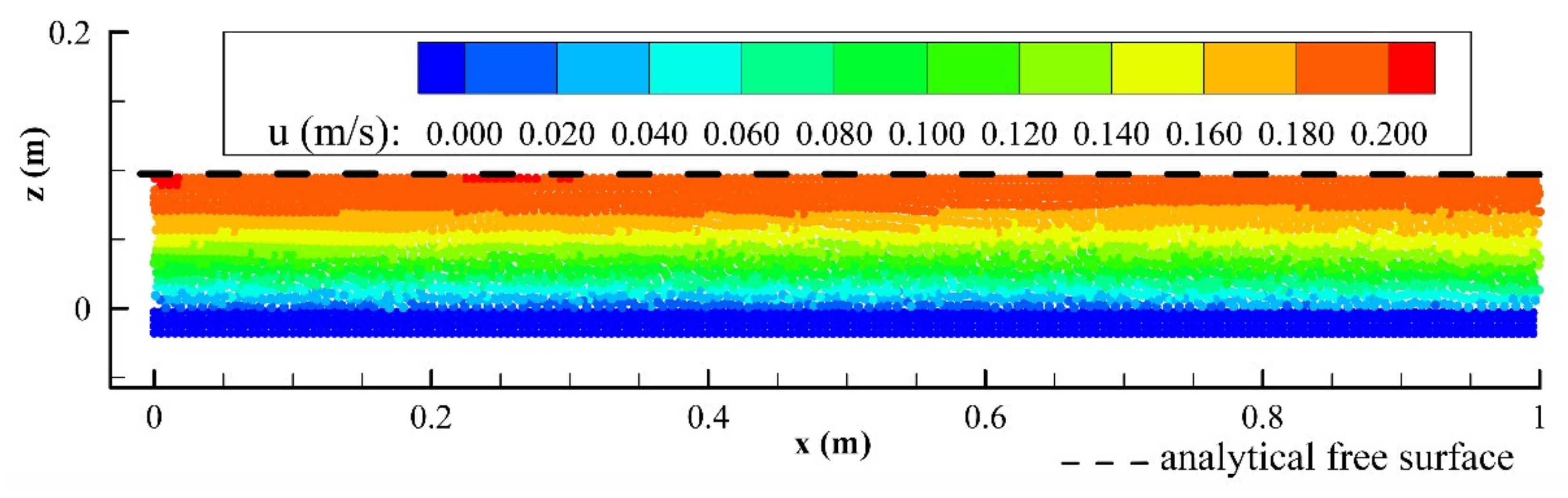
Figure 4 compares the velocity profile between the numerical results with different particle spacing and analytical solutions. The numerical results with a particle spacing
h/Δ
x = 20 show a good agreement with the analytical solutions. Therefore, the particle spacing should ensure that the particle numbers along the water depth are not less than 20.
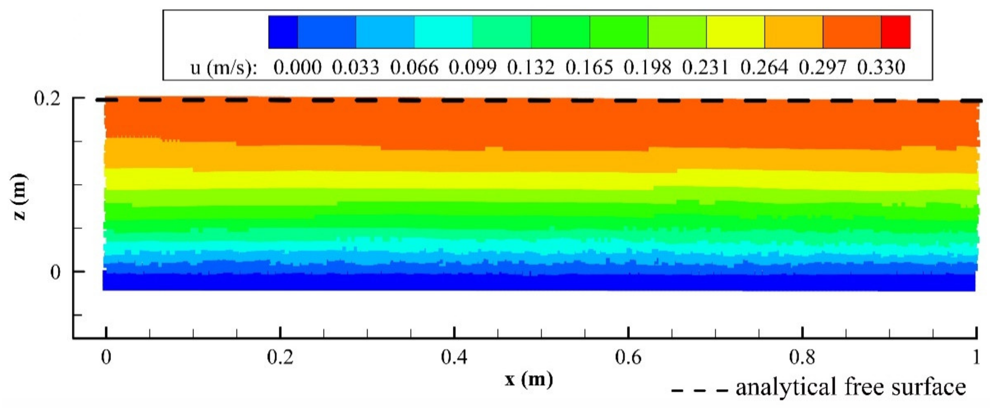
Figure 5 and
Figure 6 show the stable velocity fields of case 1 and case 2, respectively. The channel length of 1.0 m does not include the development area of the outlet and inlet flow. The wall boundary particles are shown in these figures. The numerical results show a uniform distribution for the velocity. Meanwhile, the calculated water level in channels is consistent with the analytical free surface. Similar results of flow pattern were achieved by Federico et al. [
9] and Tan et al. [
18]. In addition, quite smooth pressure fields were also obtained. The results suggest that the influence of a Shepard filter on open channel flow is not obvious.
To analyze the numerical results quantitatively, comparisons of the velocity profiles between numerical results and analytical solutions of case 1 and 2 were made, as depicted in
Figure 4. The numerical velocity profiles with
h/Δ
x = 20 show good consistency with the analytical data. The numerical results of the velocity in
Figure 4 are average values of a series of the cross-section in the calculation domain. The
L2 errors between the analytical and numerical velocity are given in
Table 1. The
L2 errors with
h/Δ
x = 20, which is less than or equal to 0.05, are quite small. This suggests that the present SPH model can accurately simulate the uniform laminar flow
where
N is the simple numbers;
and
are the numerical result and the analytical solution at position
i, respectively.
3.3. Hydraulic Jumps
To validate the model, two test cases of hydraulic jumps [
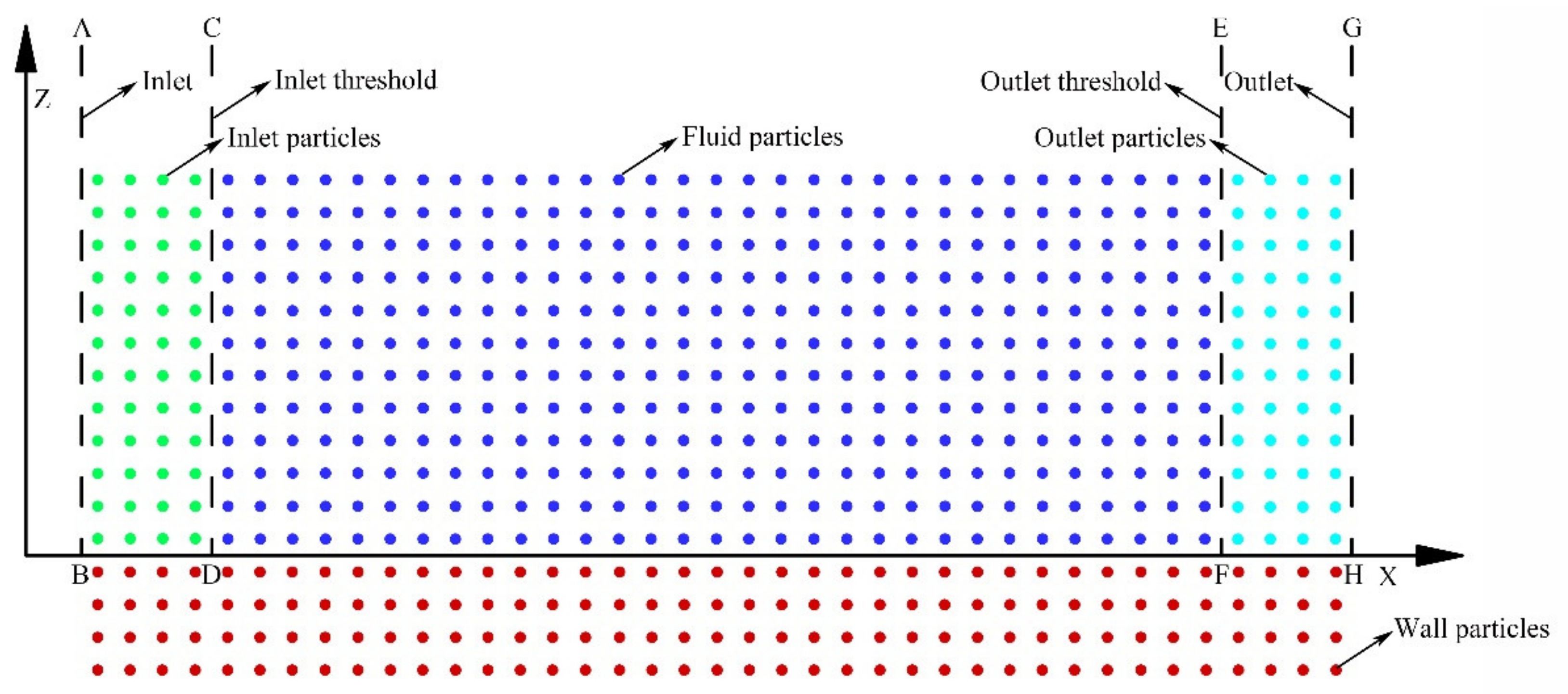
9] were selected to compare the numerical conjugate water depths with the analytical data that were calculated by the conjugate depth formula for ideal fluid. The inflow Froude numbers were
= 1.15 for case 1 and 1.88 for case 2. The corresponding types of hydraulic jumps were set to undular jump and full jump. For all the test cases, the inlet water depth
h1 was always 0.01 m. The outlet conjugate water depths obtained from the analytical formula were 0.012 m and 0.022 m for case 1 and case 2, respectively. The length of the numerical horizontal flume was
L = 40
h1. The inlet boundary conditions were specific uniform velocity
U1 and water depth
h1. The outlet boundary conditions were specific uniform velocity
U2. For the solid wall boundary, the slip boundary condition was adopted. The initial water level and velocity in the computational domain were specific uniform velocity
U2 and water depth
h1. The initial pressure and density were calculated based on the hydrostatic pressure hypothesis. For ideal fluid, the viscosity was ignored. Therefore, the model was extended to simulate the inviscid flow by replacing the dynamic viscosity with an artificial viscosity coefficient. This artificial viscosity was mainly adopted to keep stability of calculation. Here, a formula
was used. Following the study of Federico et al. [
9],
α = 0.02 was taken. It was found that the pressure fields were noisy when the
Fr1 was large. This noisiness of pressure fields was not found in Federico et al. [
9], because only velocity fields of hydraulic jumps were provided, while pressure fields were not considered. Therefore, a Shepard filter was introduced into the model. To reduce loss of time, the Shepard filter was calculated every 30-time step, which proved to be sufficient [
19]. The equation is
where
. The space between particles was 0.005 m. Total time of 16 s was simulated.
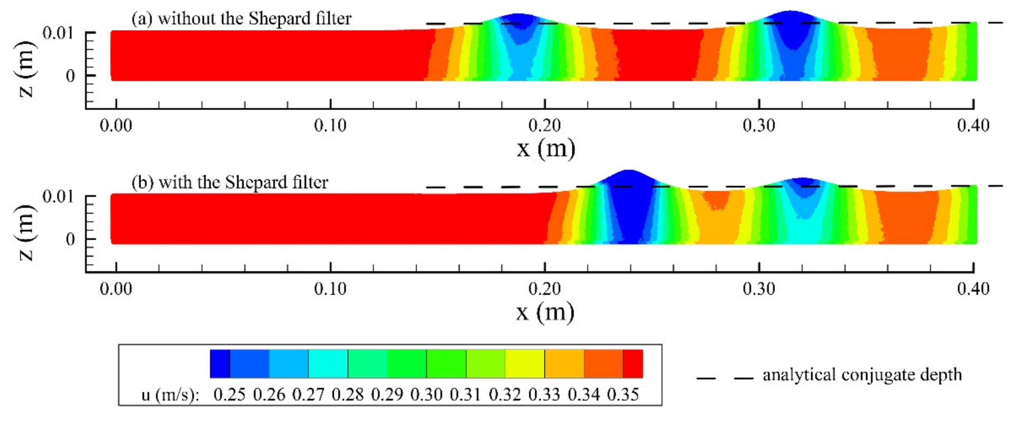
Figure 7 shows the velocity fields of case 1 at
t = 15.96 s. This time instant was approximately identical to the time used in [
9].
Figure 8 shows the pressure fields of case 1 at the same instantaneous time. The velocity fields without the Shepard filter yielded results that were similar to those of Federico et al. [
9]. Both water depths at the outlet boundary with and without the filter displayed good consistency with the analytical conjugate depth. All the four wave crests showed an overprediction with the errors of 0.002 m, 0.0025 m, 0.0035 m, and 0.0015 m, respectively. For the calculated results without the Shepard filter, the first wave crest was slightly lower than the second one. This phenomenon does not coincide with the general characteristics of undular hydraulic jumps, which display free surface undulations of decreasing amplitude [
8,
20]. The results with the Shepard filter displayed a free surface undulation with decreasing amplitude. Comparing the results of
Figure 7b with those of
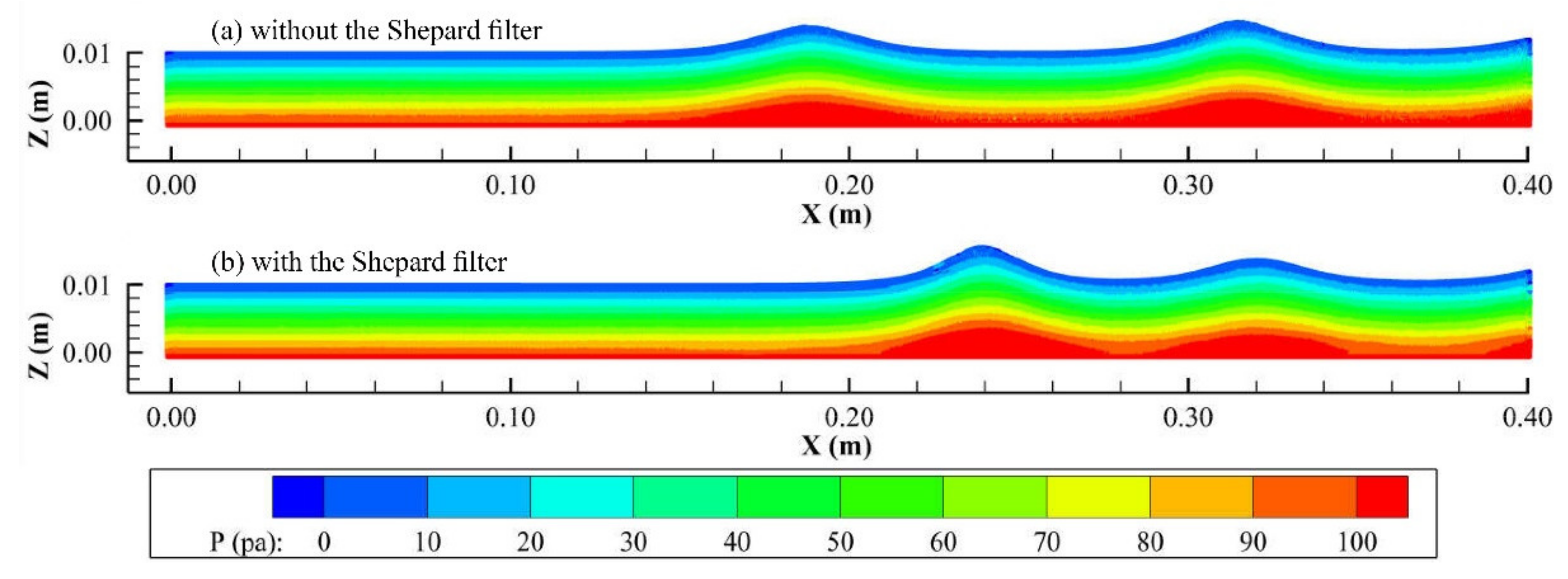
Figure 7a, the first crest with the filter is higher than the one without the filter, while the second crest is the opposite. In addition, the results with the Shepard filter display a shorter distance between the two crests than those without the Shepard filter. The pressure fields of case 1 at
t = 15.96 s are shown in
Figure 8. Both the field results with and without the Shepard filter show a uniform distribution of pressure. Thus, the Shepard filter does not obviously improve the pressure fields for a low
Fr1.
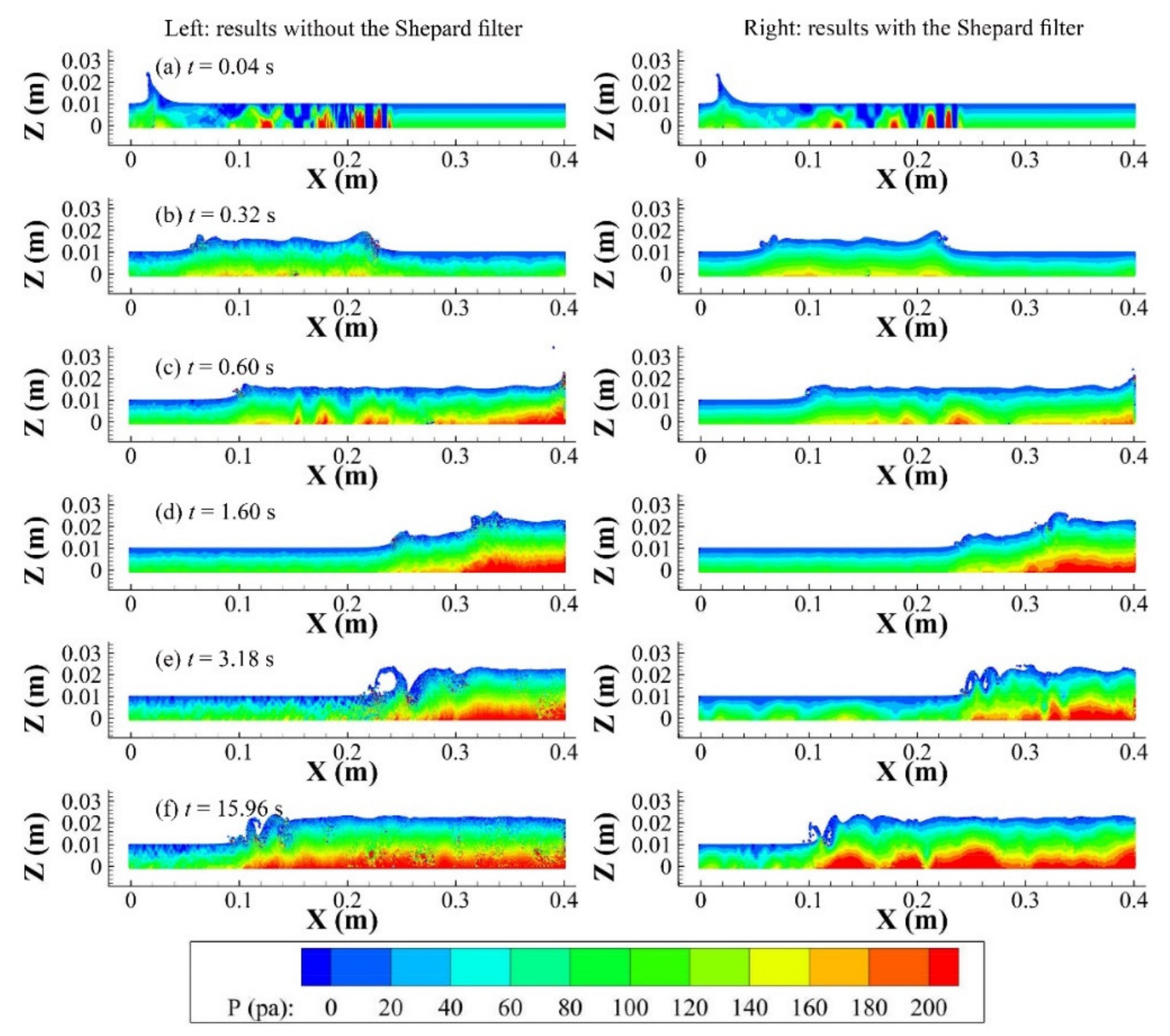
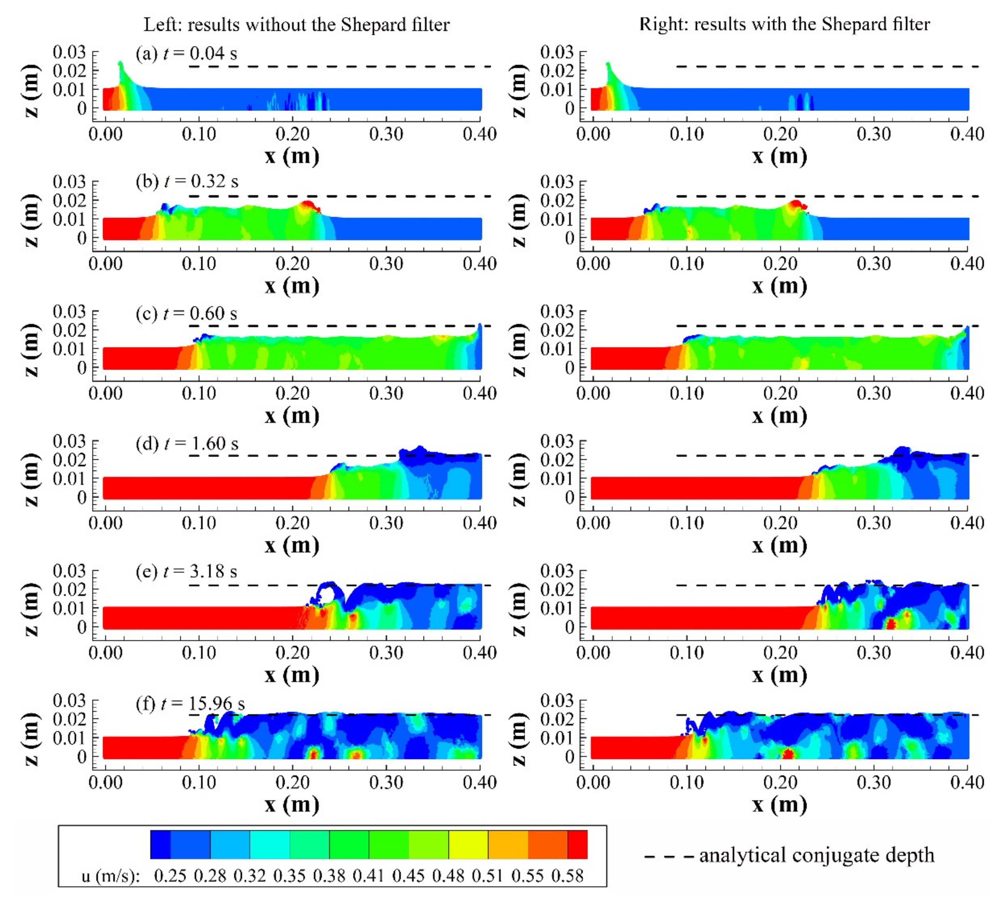
The velocity fields of case 2 at certain instantaneous times are shown in
Figure 9. The flow patterns of the two sets of results with and without the filter are similar. The inflow with larger speed interacts with the initial slow flow and hydraulic jumps at
t = 0.04 s. At
t = 0.32 s, two shock waves are formed and propagate downstream with distinct velocities. Until
t = 0.6 s, when the faster shock wave arrives at the outlet boundary and reflects upstream. The reflected wave merges with the slower shock wave and propagates continuously upstream at
t = 1.6 s and 3.18 s. The flow fields essentially achieve dynamic stabilization when the jump toe oscillates around
t = 0.1 m. In addition, the results with the filter show slightly smoother velocity fields in
Figure 9. The calculated conjugate depth with the filter is more consistent with the analytical conjugate depth than that without the filter when the flow reaches a quasi-static state.
In
Figure 10, pressure fields of case 2 are given. The pressure fields without the Shepard filter are noisy while the pressure fields with the Shepard filter exhibit much more uniform and smoother results during the entire simulation. Meanwhile, the pressure fields evolve into relatively uniform fields after a short time of about 0.32 s.


