Machine Learning Applications of Convolutional Neural Networks and Unet Architecture to Predict and Classify Demosponge Behavior

Abstract

Biological data sets are increasingly becoming information-dense, making it effective to use a computer science-based analysis. We used convolution neural networks (CNN) and the specific CNN architecture Unet to study sponge behavior over time. We analyzed a large time series of hourly high-resolution still images of a marine sponge, Suberites concinnus (Demospongiae, Suberitidae) captured between 2012 and 2015 using the NEPTUNE seafloor cabled observatory, off the west coast of Vancouver Island, Canada. We applied semantic segmentation with the Unet architecture with some modifications, including adapting parts of the architecture to be more applicable to three-channel images (RGB). Some alterations that made this model successful were the use of a dice-loss coefficient, Adam optimizer and a dropout function after each convolutional layer which provided losses, accuracies and dice scores of up to 0.03, 0.98 and 0.97, respectively. The model was tested with five-fold cross-validation. This study is a first step towards analyzing trends in the behavior of a demosponge in an environment that experiences severe seasonal and inter-annual changes in climate. The end objective is to correlate changes in sponge size (activity) over seasons and years with environmental variables collected from the same observatory platform. Our work provides a roadmap for others who seek to cross the interdisciplinary boundaries between biology and computer science.

1. Introduction

How animals react to their surroundings is a complicated function of physiology, anatomy, and life history traits [1,2,3,4]. As access to and ease of acquisition of large complex data sets has increased, complex automated analyses of an animal’s behavior has become feasible and even essential [4,5,6,7]. In terrestrial ecology, long-term ecosystem and biodiversity monitoring using trap cameras has been extensively used in wildlife studies to understand the home range, foraging and reproductive behavior of animals [8,9,10]. More recently, advances in permanent ocean observatory infrastructures brought this option to the seafloor allowing further understanding of how benthic species, including those in deep-sea environments, respond to diel, seasonal and inter-annual environmental variability [11,12,13]. In some instances, nearly 15 years of video imagery acquired from these networks raise a challenge of transforming the petabytes of pixel-based information into ecological semantics and ultimately, knowledge [14,15,16].

Big data and biological monitoring pose major issues. Each ecosystem and each taxonomic grouping presents its own unique set of challenges. Benthic marine organisms are among the more difficult groups of animals to monitor. They tend to be small, often live in difficult to access areas, and have behaviors generally on a very different temporal scale from those of terrestrial animals, for which much of the pioneering monitoring work was performed. For example, extremes of the temporal scale of behaviors in marine invertebrates range from the snapping punch of the mantis shrimp that boils the water in front of it in milliseconds [17], to the slow stroll of a sea urchin on its tube feet along the ocean floor, for hours or days [18]. To understand these activities in the context of the animal’s ecology, heterogeneous data, including physical, chemical and biological variables need to be acquired over the same time period. The relevant information in these data can only be fully accessed using the appropriate artificial intelligence methodologies, which are capable of discovering underlying trends and unexpected relationships among the range of environmental and biological variables.

This investigation focuses on understanding the behavior of a sponge that has been monitored over three years by cameras at the Ocean Networks Canada Folger Observatory. Our goal is to automate the classification of sponge activity over time by using machine learning to predict the changes in its size. Previous analyses of sponge behavior have largely used software such as ImageJ, with few attempts to use machine learning methods [19,20,21]. No other work has generated an automated method that can extract complex colored objects from a changing colored background over time.

Video and still image data of benthic communities acquired over long periods, and which include seasonal variations, contain a lot of information that is not readily usable. Image processing algorithms can detect and sort the relevant content. For example, the activity of animals living on the seafloor should be considered in the context of the substrate they are attached to or moving across. In this case, image processing algorithms should be capable of discriminating between foreground image regions containing the subject and background areas that are not relevant, and in some cases, both may be of interest. Many computer vision approaches exist for image segmentation [22,23], but efficient and effective results can be obtained by using supervised machine learning approaches [24]. Semantic segmentation is a class of machine learning in which each pixel is given a label identifying it as a member of a particular class, background and foreground [25]. Other machine learning methods vary from simple image classification such as object detection or instance segmentation, to whole image classification with multiclass identification, such as instance segmentation [26,27,28].

The application of image classification from a machine learning perspective is used to select specific aspects out of images that contain large amounts of data both in terms of quantity and variety (e.g., color and texture in both foreground and background aspects). In this investigation we aim to isolate the image of a sponge from a complex background in which the sponge and background change over seasons and years. We have two objectives: we first clearly outline a methodology using convolutional neural networks with large image data sets that is effective for use by other biologists and ecologists; next, we apply this approach to study the behavior of a sponge in situ to provide an example of how this type of machine learning is applicable to a range of image sets.

2. Materials and Methods

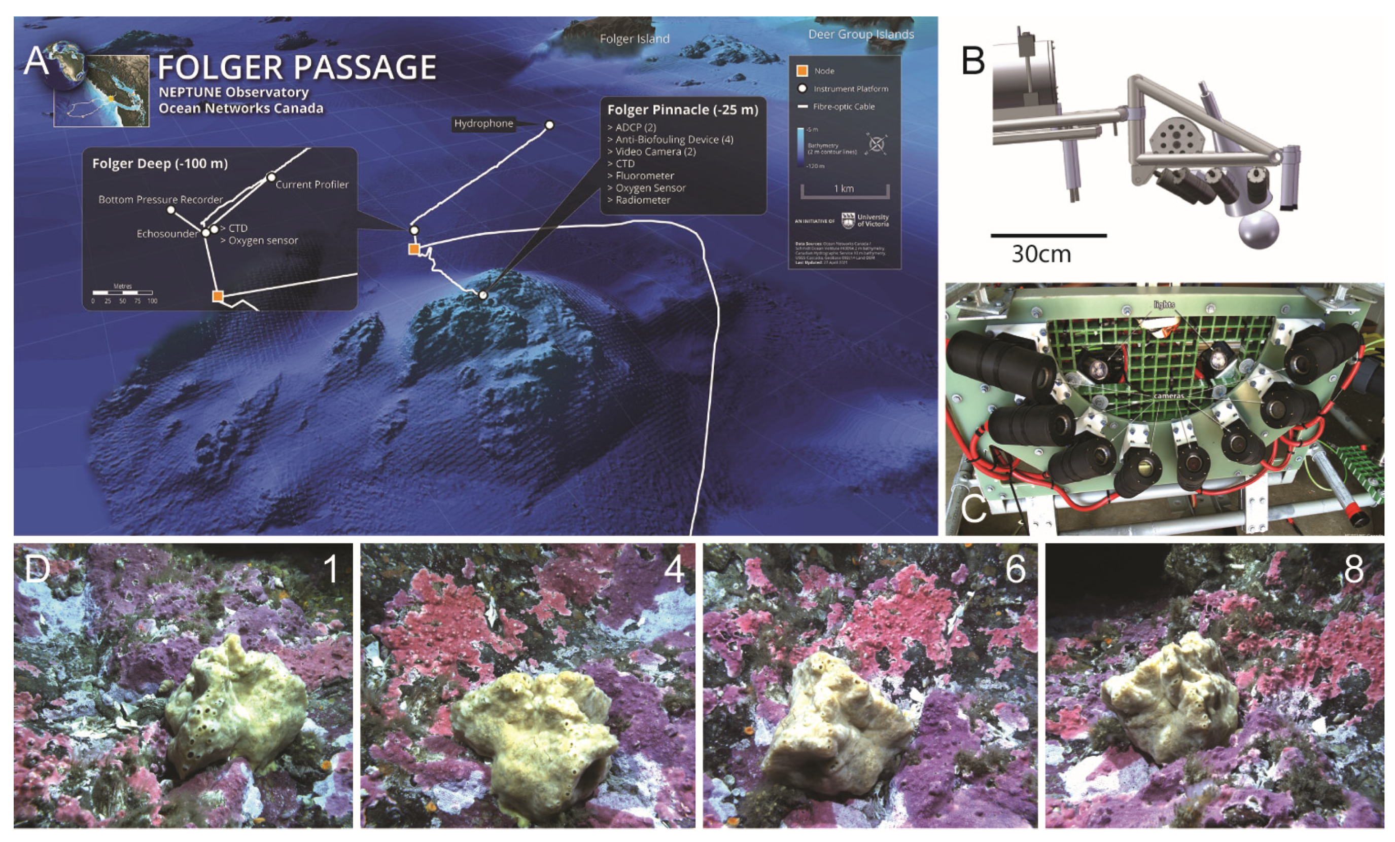
2.1. Study Site, Video Imagery and Environmental Data Acquisition

Data were collected from an underwater platform connected to the Ocean Networks Canada NEPTUNE cabled observatory (https://oceannetworks.c, accessed on 20 June 2019). There are two oceanographic instrument platforms at this site, Folger Pinnacle and Folger Deep at 23 m and 100 m respectively, off the southwest coast of Vancouver Island (Figure 1). The location is 10 km west of the Bamfield Marine Science Center (BMSC) in British Columbia, Canada, at the entrance to Barkley Sound. Both video imagery and ancillary oceanographic data collected for this study were from the Folger Pinnacle platform. The environmental parameters of interest, all measured at a 1 Hz sampling frequency, were temperature, salinity, photosynthetically active radiation (PAR), current direction and velocity, chlorophyll content and ambient pressure. A video camera system was positioned to observe a fist-sized demosponge, Suberites concinnus. The system was in fact an eight-stage camera array evenly distributed around a 30 cm radius semi-circle (180°) allowing 3D image reconstruction [29]. Two LED lights with a combined 400 lumen output provided illumination during video recording (Figure 1). Between 2012 and 2015 six different still image time lapse series with images captured each hour were collected (TL1 to TL6;

Table 1. Dates during which each time-lapse series occurred and number of images used for training and testing.

Time Series	Dates (DD/MM/YY)	Timeseries: Total Number of Images	Training Data: Number of Training Images and Masks	Testing Data: Number of Test Images
TL1	08/11/12–13/04/13	1072	428	644
TL2	15/07/13–10/09/13	112	46	66
TL3	20/10/13–15/12/13	968	387	581
TL4	20/07/14–21/08/14	696	278	418
TL5	01/10/14–31/01/15	1932	772	1160
TL6	15/07/15–15/08/15	316	126	190

).

Periodically, the image quality deteriorated due to biofouling (growth of barnacles mostly) on the camera lenses, therefore requiring a manual cleaning schedule using SCUBA divers. Since maintenance of the subsea infrastructure was dependent on weather conditions, camera cleaning took place at irregular intervals. Quite noticeably, biofouling occurred faster after cleaning took place in late spring or summer. This generated variable lengths in TL1–TL6 video times-series periods (Table 1). Variable biofouling patterns among the different cameras also forced the selection of a single camera (Camera 8, Figure 1), which was the least affected by growth, and therefore, generated the highest number of high-quality images. The demosponge was the focus of this project’s longer-term aim to understand the sponge’s behavior with respect to the range of environmental parameters it experienced (Figure 1).

This specimen of demosponge, S. concinnus, was nicknamed ‘Belinda’ for ease of reference and is referred to by that name hereafter. One of the primary objectives of this investigation was to classify and map the different behaviors of Belinda. Belinda shows a variety of movements, both long-term and short-term. For example, over the winter months we observed a type of torpor behavior in which the sponge contracted to about a third of its original size. In all time series that included winter months, the sponge’s movement was minimal from December through February (observed in TL1;

Table 2. Performance of the model for each time lapse series at the 50th epoch. Loss, dice score and accuracy.

Time Series	Loss	Dice-Coefficient Score	Accuracy	Validation Loss	Validation Dice-Coefficient Score	Validation Accuracy
TL1	0.0300	0.9700	0.9862	0.0505	0.9477	0.9619
TL2	0.3417	0.6794	0.9176	0.2603	0.7397	0.8597
TL3	0.0629	0.9375	0.9788	0.1328	0.8680	0.9473
TL4	0.0575	0.9425	0.9627	0.0685	0.9309	0.9590
TL5	0.0447	0.9553	0.9777	0.1140	0.8863	0.9429
TL6	0.0779	0.9233	0.9646	0.6250	0.3696	0.3465

). Some behaviors documented in demosponges previously include twitches (isolated and localized contractions on one side of the body), ripples (a wave-like contraction with a series of contractions along the body in a sequential pattern), and cringes (whole-body contractions) [21,30]. We observed and documented many instances of similar behaviors by Belinda in each of the six time-series.

The convolutional neural networks were built using Python 3.8.8. Packages were installed and imported using a Jupyter notebook 3.6 interface and Anaconda 4 as the Python distributor. The following packages were used to build and create the model: TensorFlow 2.5, Keras 2.5, and Open-CV2. The code developed for this paper and instructional material is available on a Github repository [31].

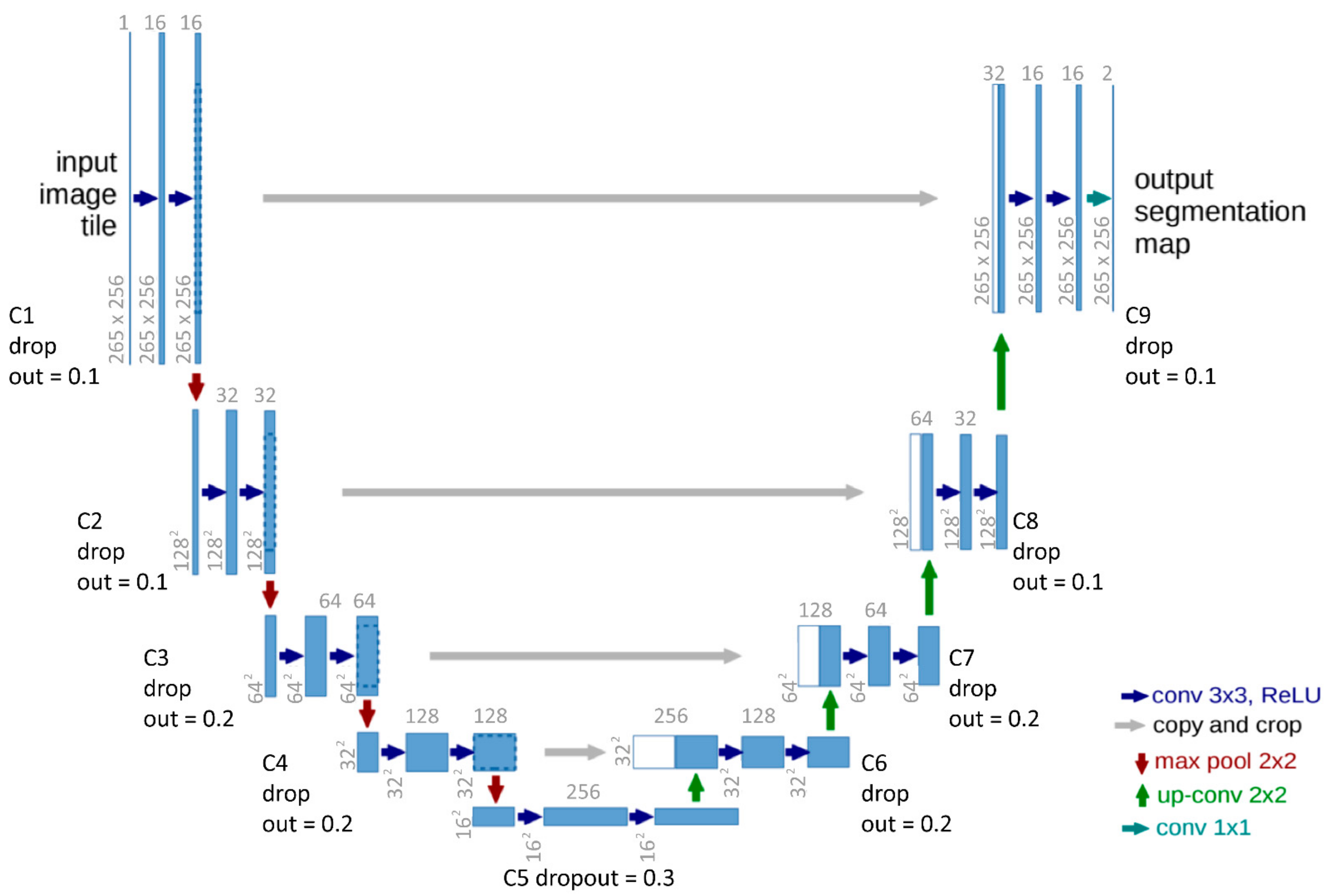
2.2. CNN and Unet Explanation

We approached the process of behavior classification using image segmentation. We classified the entire image and identified two classes: sponge and not sponge. As seen in Figure 1D (lower row of images), the backgrounds of the images are complex, with many colors, shapes, and a range of brightness across the field of view. The background is also very dynamic, with many other benthic organisms moving in and out of the scene. Between the complex background, variety of behaviors, and the extensive temporal dimensions of the data set, we decided to use a machine learning (ML) approach based on the Unet architecture for our convolutional neural network (CNN) analysis.

For each layer there is the pixel size (for example 256 × 256) and the dimension depth of applied features/filters (for example the 16 in C1). Conv 3 × 3 ReLu is the activation function within each layer. The ‘copy and crop’ is the concatenation of the contracting (encoder) path to the expansion (decoder) path. The max pool layer of 2 × 2 is the size of the filter applied at each layer. A detailed explanation is found in Section 3.1 CNN and Unet explanation. The original diagram from Ronneberger et al. [32] was modified to demonstrate the alterations for this investigation (Figure 2).

Raw images of Belinda are shown along with their corresponding manually created masks (ground-truthed masks) and predicted masks (output/classification of the model) for TL1, TL5 and TL6 (Figure 3). Columns are different groups of image types through the project (left to right: raw images, masks and predicted mask) and the rows are the three time series that were used as examples. (B) A bar chart displays the total number of images for each time series from panel A. The time series is on the x-axis and total number of images is on the y-axis. (C) A bar chart shows the dice coefficient loss of the predicted masks for TL1, TL5 and TL6. The time series is on the x-axis and the loss is on the y-axis.

Many architectures have been developed for neural networks and it is even possible to develop a novel neural network unique to a specific data set. Some conventional and popular CNN architectures come with their own libraries, such as VGG, google LeNet, ResNet13, or Inception V3. Since our sponge behavior question required all the pixels in the image to be defined, the approach we settled on was semantic segmentation. Therefore, we needed a CNN architecture designed for imagery with all the pixels classified. In our case, there are two classes: ‘sponge’ and ‘not sponge’. The CNN architecture Unet was originally designed for grey scale (one channel) biomedical image segmentation from microscopy data sets [32]. It has since been applied to many other biological applications, including coral identification or changes in size of sponge under a similar deep sea observation platform context in colored images (RGB or three channels) [33,34].

Semantic segmentation is similar to traditional image analysis used in remote sensing applications where each pixel is given a label or class. Unet is designed specifically for semantic segmentation and works best with two classes and whole image labeling. The architecture of Unet is in the shape of a U where there are two paths: a contraction or encoder path and an expansion or decoder path. Each encoder convolution layer is concatenated to its reciprocal decoder layer (Figure 2). Each concatenation provides a localized feature specific for the segmented classes. We modified the original architecture of the Unet classification to fit our questions better (Figure 2). For example, Unet was designed with greyscale imagery, and our color images have three channels, RGB.

The basic concept behind the Unet deep learning technique is to use convolutional layers and max-pooling architectures to extract identifying features and patterns from a series of images. The input layer for this investigation was 256 by 256 by 3 (Figure 2). The images were resized to 256 by 256, and the three channels indicate that they are color images (red, green, and blue RGB; Figure 2). In a CNN model, the convolutional layer is a series of filters compiled together by convolution responses. After using these compiled filters, we used max-pooling in which a smaller matrix (e.g., 5 by 5, or 3 by 3 kernels) is run over the convolutional layer at a specified stride such that one step (or pixel) would be a stride (stride = 1) (Figure 2). The 2D convolutional layering and max-pooling are repeated many times to increase the dimensions of the image. The type of architecture used determines how many layers and max-pooling events are applied and vary in the number of dimensions, eventually obtaining what is known as the dense layers, where there are many neurons connected to each other which ultimately determines the size and shape of the output layer.

2.3. Running the Model

2.3.1. Preprocessing of Images

To prepare the images for use in the model, several preprocessing steps were needed. First, the images were cropped from 2448 by 2048 pixels to 1500 by 1500 pixels images. This was performed to reduce the amount of distortion when applied to the CNN model (CNN requires a square input image), and it reduced unnecessary noise of the ‘not sponge’ class that would come from a dark region in the top left quadrant of each image caused by the position of the underwater lights relative to the camera’s view of the sponge.

A vital step in training the model to perform predictive analyses is ground-truthing. Ground-truthing is the preparation of a set of measurements that are a known accurate representation of the classes within the image. Ground-truthed images are used to train the model. We randomly selected 40% of each time series and manually drew a polygon around the sponge in the image. The interior of the polygon was classified as ‘sponge,’ and the exterior as ‘not sponge’. This was accomplished with a Matlab application called ‘image labeler’ [35], and labelled images were exported as binary masks classified as a 1 or 0, ‘sponge’ and ‘not sponge,’ respectively. In Figure 3 the last row of images illustrates the output of the model with an example from three of the time series.

2.3.2. Processing: Unet Modification and the Steps to Running the Model

Images were resized to 256 by 256 height and width with three channels (RGB). This step is necessary to fit into the architecture of Unet. The data were divided into training subsets with corresponding masks and a testing data set containing all the other images in the time series. For each time series, we divided the data into 40% for training and 60% for testing (Table 1; last two columns). We chose to perform this for each series because of the seasonal changes in the appearance of the sponge which suggested to us that the training data set more closely representing the test data set might perform more accurately. A portion (40%) of the images were masked and used to train the model and the rest of the data was used as the test data (Table 1). The training data were used to train and validate the model and the test data were used to test the performance of the model. Additionally, the testing was used to provide a predicted area of the two classes, ‘sponge’ and ‘not sponge’ over time (Figure 3). We used Keras application programming interface (API; https://keras.io/, accessed on 21 January 2019) and Tensorflow 2 libraries (https://www.tensorflow.org/, accessed on 21 January 2019) for this machine learning model.

For our modified Unet model we used a rectified linear unit (ReLu) with a 3 by 3 kernel for the convolutional operations. Our max-pooling matrix was 2 by 2 where the maximum value is selected and replaced the matrix with this value. We used the padding functionality provided by the Tensorflow libraries to ensure the output dimensions were equal to the input dimensions. We used He-normal kernel initializer for the starting weights (a truncated gaussian distribution; [36]). For the optimizer, we used Adam and dice-coefficient loss for our loss function [37,38,39]. The original Unet architecture published by Ronneberger et al. [32] did not use the padding function and it used normal distribution for their starting weights, stochastic gradient descent for the optimizer and a cross-entropy loss function.

We had five contracting (down sampling) convolutional layers with a 0.1 dropout for each layer. The dropout function randomly removed 10% of the neurons (connections between layers) to prevent overfitting. For each layer, the dimensions were halved, and the channels were doubled (Figure 2). For example, from C1 to C2: 256 × 256 × 3, the output is 128 × 125 × 6 (Figure 2). Next, there were five expanding (up-sampling) layers; each was a reciprocal of its counterpart down-sampled layer. For example, as seen in Figure 2, layer C4 is the reciprocal to U6. The difference between the up-sampled layers and the down-sampled layers is that we added a concatenation of the down sampling layer, as seen in Figure 2, U6 = U6 + C4. The output of C4 was added to U6.

We trained the model using the randomly selected subset of images and masks (40%) described above to obtain the total trainable parameters. After the model was trained, the model was applied to the rest of the images. We ran the predicted model sequentially over all the images in each time series for a total of six models trained and fitted (TL1-TL6; Table 1). We ran 50 epochs, where one epoch is one full feed-forward and feed-backward, or one down-sampling and then up-sampling. We used a 0.2 split for validation and had a batch size of 16. Moreover, we used checkpoints with the Keras library to save the model if the model fails. The ‘save best only’ checkpoint was used because it saves the best model according to the quantity monitored and prevents overfitting (TensorFlow). We used callbacks to save at specific stop points along the model. We used ‘early stopping’ to prevent overfitting. This callback was to monitor validation loss; if there is no change in the validation loss over three epochs, it stops the model early. It stops if this is the case because it is assumed this is the best that can be achieved. To run the model, we created a threshold of 0.5 for each group of data to make sure the outputs were binary.

2.3.3. Post-Processing

For the performance of the models, we reported the accuracy, dice-coefficient score and the loss and the validation accuracy, validation score and validation loss (Table 2). The accuracy is the mean percentage of correct predictions, the dice coefficient score is the precision of the model or the amount of overlap between the actual class and the predictions, and the loss is the mean error rate. The validation accuracy, score and loss are all the same as previously described, however it does not use the updated weights at each epoch (time of the model), meaning is it a validation built into the model at each epoch to prevent overfitting. If the validation values are very different from the model values (accuracy, score and loss; ASL) this suggests overfitting occurred. These error and model performance statistics are standard for evaluating machine learning applications [40].

A K-fold cross validation was performed on each time series model (TL1–TL6). This was accomplished in Python 3.8.8 using tensor flow 2.5.0, Keras 2.5 and sklearn model selection K-fold (scikit learn 0.024.2). For this validation procedure specifically, we used a five-fold cross validation. The data which we originally used to train the model (the randomly selected 40% and ground-truthed images) were split into five equal parts or also referred to as five consecutive folds. Each fold was used once as a validation while the remaining folds were used to train and run the model [41]. The model was run five times and each time the accuracy and loss were calculated. For each time series and cross validation three figures were produced: training and validation loss curves (i.e., learning curves; Figure 4), training and validation accuracy curves (i.e., learning curves; Figure 5) and a confusion matrix (Figure 6).

The learning curves show change over time in the learning performance of the model. They are diagnostic tools in machine learning models to demonstrate the goodness of fit (i.e., if there was any overfitting or underfitting of the model) and if the validation data are representative of the training data. A learning curve indicates underfitting if the loss continues to decrease at the end of the training or the loss remains flat regardless of training. The learning curves show overfitting if the loss decreases and then at the end of the training begins to increase. A good fit for learning curves is when the loss (or accuracy) reaches a point of stability or there is a small gap between the validation and training curves (Figure 4 and Figure 5).

For the cross-validation, a simple confusion matrix was produced for each with predicted labels on the x-axis and true labels on the y-axis (Figure 6). The top left and bottom right quadrants indicate the accurate predictions, and the top right and bottom left quadrants indicate the incorrect predictions (Figure 6). We used an SNS heatmap from the package Seaborn 0.11.1 to present the correctly and incorrectly identified pixels from the five-fold cross validation. The heat map is broken down into four quadrants: the top right quadrants are the true negatives or correctly identified ‘sponge’ class, the top left quadrants are the false positives where ‘not sponge’ is misclassified as ‘sponge’, the bottom left quadrant is the false negatives where ‘sponge’ is misclassified as ‘not sponge’ and the bottom right quadrants are the true positives or the correctly labeled ‘not sponge’ class (Figure 6).

The top-left quadrant of each graph shows the true negatives, the bottom right quadrant shows the true positives, the bottom-left quadrant shows the false negatives, and the top-right quadrant shows the false positives. Numerical values on the y-axis represent the number of pixels for each classification type, true positives/negatives and false positives/negatives. Dark colors represent lower values of pixels and light colors indicate higher values of pixels for each classification type. The two classes of pixels we used were ‘sponge’ and ‘not sponge’. False positives and negatives are in the quadrants where the classes do not match (example sponge, not-sponge bottom left quadrant) and true positives and negatives are in the quadrants where the classes matchup (example: sponge-sponge bottom right quadrant).

3. Results

3.1. Model Architecture

The architecture of the model had a total of 1,941,105 trainable parameters and zero non-trainable parameters. There were five contraction paths and five expansion paths, the drop out for C1–5 had drop layers set at 0.1, 0.1, 0.2, 0.2 and 0.3 respectively. C6–9 layers had drop out layers set at 0.2, 0.2, 0.1, and 0.1, respectively (Figure 2). Each layer had a max-pooling layer labelled as P# with a filter of 2 by 2. In the expansion path, the concatenation is indicated by the U# (Figure 2).

3.2. Data Summary

The number of images in each time series is an important factor for the time it takes to run the model and overall goodness of fit or performance of the model. Table 1 summarizes the dates and total number of images in each time series. The time series with the most images was TL5 with 1932 images and the least was TL2 with 112 images. The descending order of the quantity of images is TL5, TL1, TL3, TL4, TL6 and TL2. This order roughly corresponds to the quality of the goodness of fit of the model and therefore we suggest that an important metric of model performance is the amount of data used. As mentioned already, we used 40% of the images in each time series to train and validate the model; therefore, the larger the training data set, the better the performance of the model.

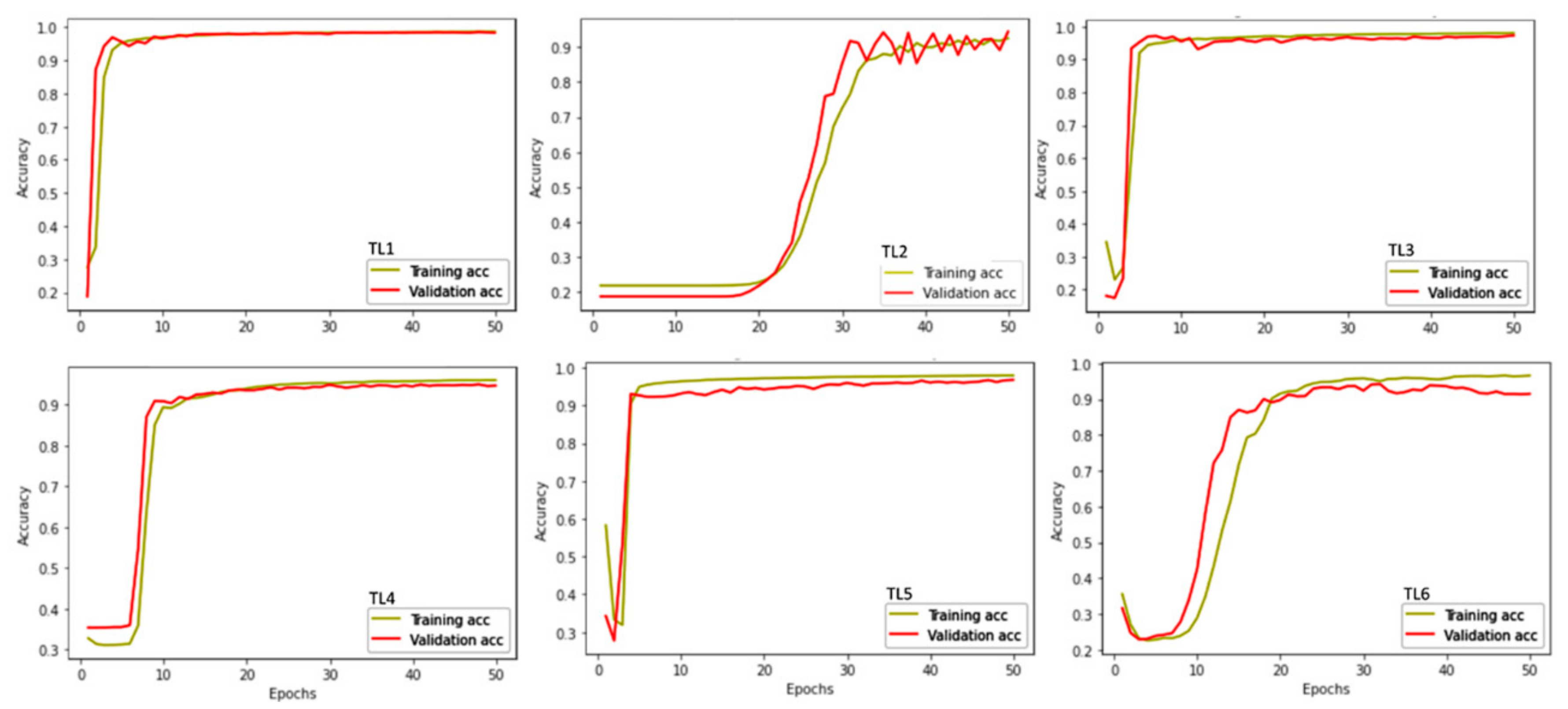
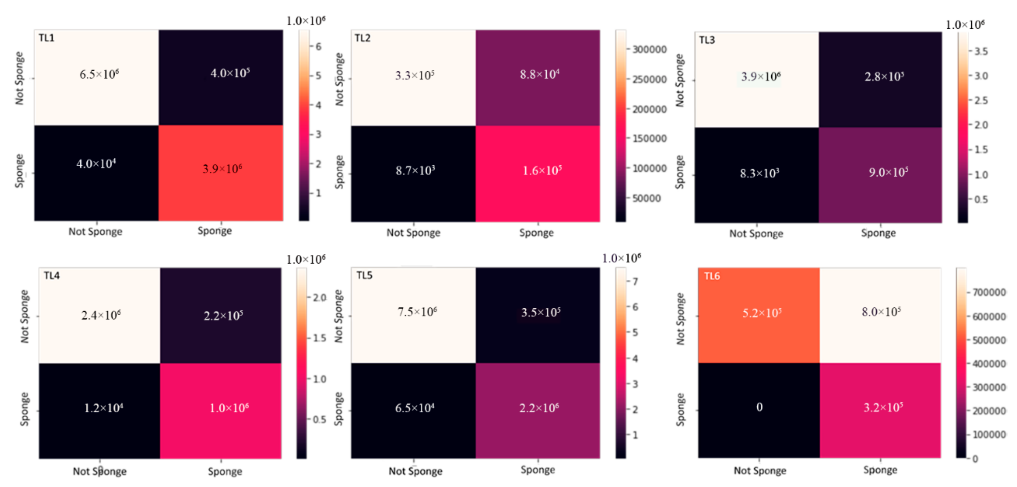
3.3. Model Performance

We ran the Unet architecture for each time series. We reported the models’ performance, the accuracy, dice-coefficient score and the loss (ASL; Table 2), as well as the validation accuracy, validation score and validation loss (validation ASL; Table 2).

The best model was TL1 (ASL: 0.0300, 0.9700 and 0.9862; Table 2) and then a close second was TL5 (ASL: 0.0447, 0.9553, 0.9777; Table 2). Surprisingly, TL4 had the closest ASL to the validation ASL scores which indicates the best goodness of fit of all the models. The worst performing models were TL6 (ASL: 0.0779, 0.9233, 0.9646; Table 2) and TL2 (ASL: 0.3417, 0.6794, 0.9176; Table 2). Moreover, TL6 and TL3 showed the most overfitting (i.e., the ASL and validation ASL were the furthest apart). The performance is likely due to the number of images in the time series, but other factors such as consistency in brightness of the images, variability between images, the number of images in which a fish was in front of the camera, or if the camera malfunctioned, also contributed to performance of the model.

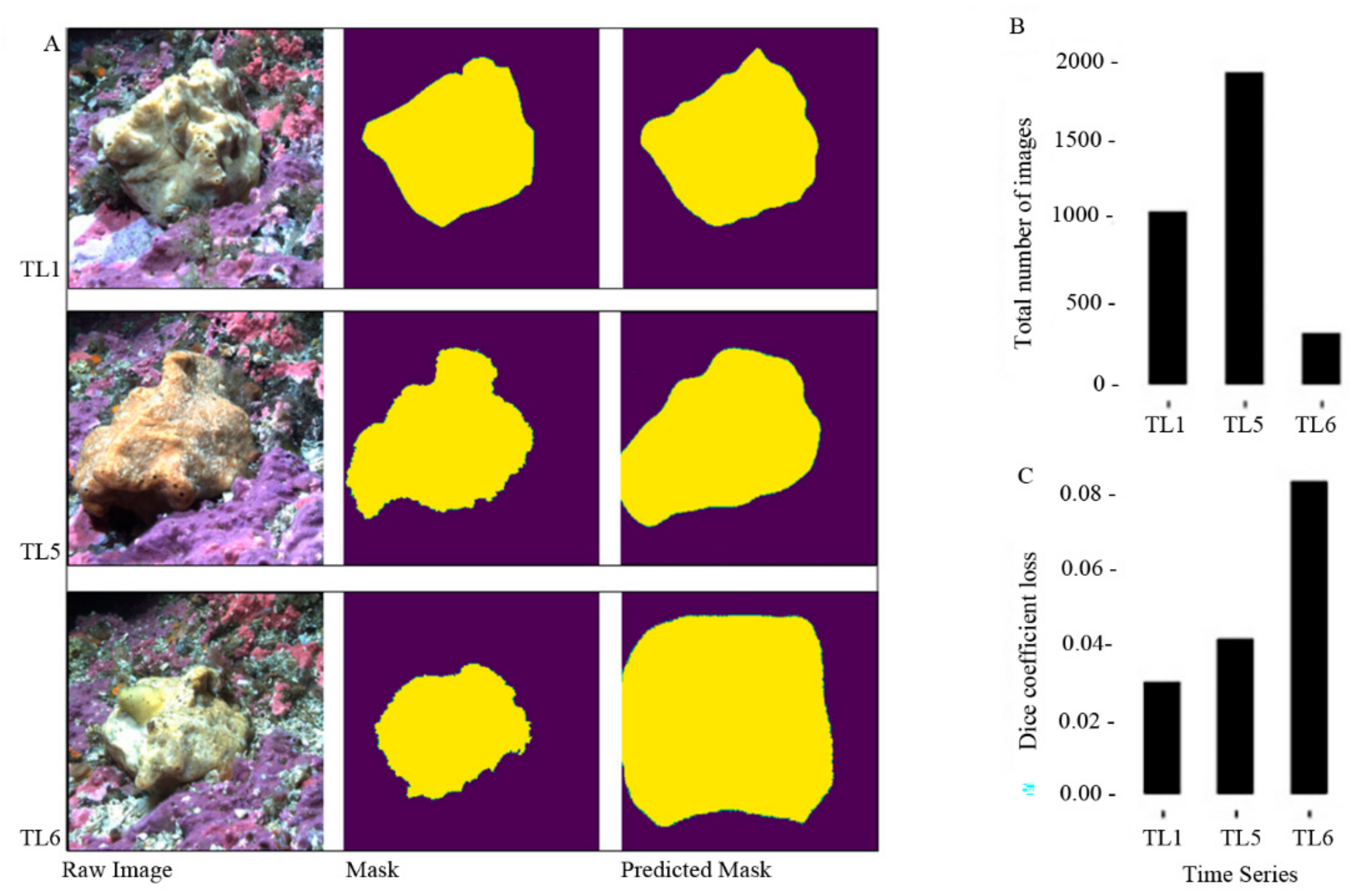
3.4. Validation of the Model

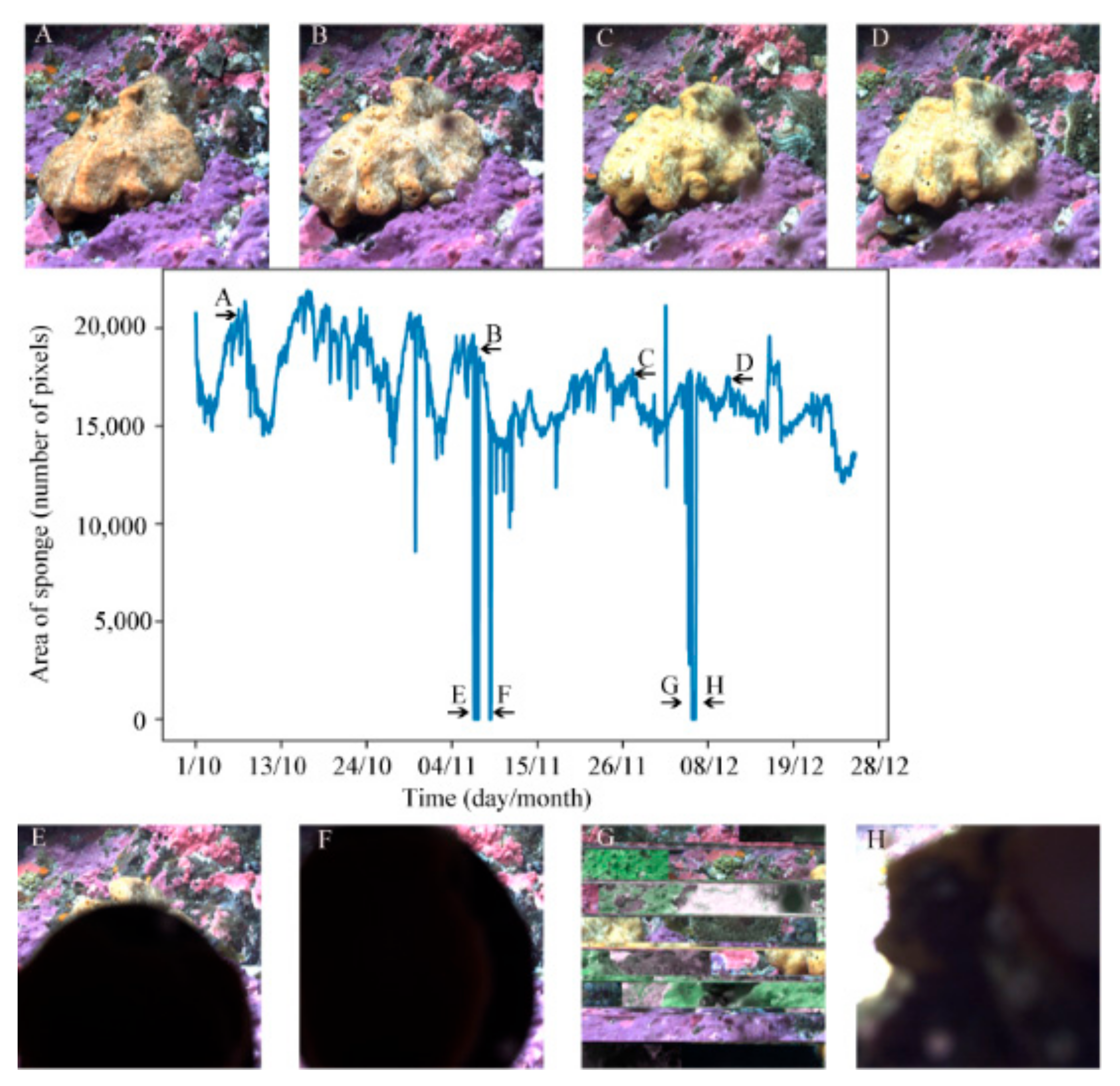
The two learning curves are the loss and accuracy learning curves over time of the cross-validation. The validation data (red lines in Figure 4 and Figure 5) should resemble the patterns observed in the training data (yellow lines in Figure 4 and Figure 5) to show that the model is not over or underfitting. More specifically, for the accuracy learning curve should be exponential growth and a plateau. The loss learning curves should have exponential declines followed by stabilization.

In the accuracy learning curves we see that TL1, TL3, TL4 and TL5 all demonstrate an ideal goodness of fit (Figure 4). Whereas TL2 and TL6 are slightly different. TL2 is noisy at the end of the model (higher epochs) and in TL6 the accuracy started to decrease over time; both of these trends are indicative of some overfitting (Figure 4). In the loss learning curves, we see that TL3, TL4 and TL5 all demonstrate a good-fit curve (Figure 5). TL1, TL2, and TL6 have a fair amount of noise in the validation data (red lines in Figure 5). Both TL1, and TL6 have higher loss values, whereas TL2 validation data has a lot of noise (fluctuations). All three of these trends over time (epochs) indicate some form of unrepresentative training data (Figure 5). TL2 and TL6 support the findings from the accuracy learning curve of overfitting; however, the TL1 loss curve differs from the accuracy curve suggesting a small amount of overfitting in the model (Figure 5).

For each five-fold cross validation, the simple confusion matrix was represented using a heatmap (Figure 6). Dark colors indicate low values whereas lighter colors indicate high values. The best-case scenario is dark in the false positive and false negative quadrants (top right and bottom left, respectively) and lighter colors, high values in the true negative and true positive quadrants (top left and bottom right respectively) (Figure 6). Across all time series we see that the false positives and false negatives are dark except for the false negative in TL6 which is very light (8 × 10⁵ Figure 6). This suggests there were many false negatives in TL6, possibly because this time series had fewer images than the other time series and the overall model performance was the lowest. In all the time series, the true negatives (‘sponge’ class) performed very well because the top left quadrant for all time series demonstrates a light color. This is not the case for the background or true positives (‘not sponge’ class) where they are all some shade of pink to dark purple, possibly due to the nature of the complexity of the background (Figure 6).

In general, from these confusion matrices we can draw two main conclusions: more true negatives which mean more ‘sponge’ is being correctly identified than ‘not sponge’, and more false positives are occurring, which mean more ‘not sponge’ is being misclassified as ‘sponge’ than the false negatives.

3.5. Area over Time

The next step of this project is to analyze and classify the types of behavior shown by Belinda to identify which environmental parameters are correlated with the different behaviors. In Figure 7, we created a graph showing the change in area of the sponge in the image over time using the predicted classification for the entire time series of TL5 (Table 1). There are a few instances where the area identified as sponge is near zero (Figure 7). These points were caused by either larger organisms crawling on the sponge and changing the view, or instances in which the view of the sponge was obstructed by fish swimming in front of the camera. In Figure 7, panels E to H illustrate problems with the camera (due to the network) or a fish swimming in front of the camera compared with panels A to D of images with no disturbance to the image.

4. Discussion

4.1. Application of Biological Data Sets

We demonstrate the application of Unet, with some minor modifications to the architecture, to a large biological image data set. The original implementation for Unet was designed for biomedical applications. Our objective is to use this case study of analysis of sponge behavior to provide a roadmap for a broad range of biological applications.

There are some major advantages to the methodology we describe. First, the model can handle complex images with novel and diverse backgrounds. For example, the background of the images we analyzed had a lot of variation in the visible range as well as differences in contrast and brightness, and yet our method was over 95% accurate (Table 2). Second, the model can handle large data sets; the more data and images, the better the performance of the model. Our model showed the best performance with the largest set of images, for example TL5 (Table 1 and Table 2).

Nevertheless, there are some considerations regarding the use of this technique to answer scientific questions that we learned early on in the process of creating this methodology. For example, ground-truthing the data requires a significant initial time investment. As described above for each time series, there was a manual process of masking the two classes of ‘sponge’ and ‘not sponge’, called ground-truthing. We accomplished this by randomly selecting 40% of the images in each time series (Table 1). Another consideration is the need for a relatively large data set. The performance of the model was closely correlated with the number of images within the time series. For example, TL6 had 316 images and had a validation ASL of 0.6250, 0.3696, and 0.3465 while TL1 and TL5 had 1072 and 1932 images, respectively, with validation ASL’s of 0.505, 0.9477, 0.9616, and 0.1140, 0.8863, 0.9429, respectively (Table 1 and Table 2).

Certain parameters of data sets make this methodology more effective. The model we generated would work well for biological questions investigating data sets of time series with unique background and foreground image types, motion detection (behavior mapping), automated identification of individuals or specific identifiable parameters, or classification of groups of organisms, for example. However, there are groups of biological data sets that would not be appropriate for this methodology. For example, data with small sample sizes, single or few images with multispectral or hyperspectral features, and building maps or land use change. These types of data are more suited for traditional machine learning or classification algorithms, such as a support vector machine or a random forest decision tree analysis.

4.2. Model Performance and Alterations

We successfully demonstrated that the application of Unet can be used to solve complex biological problems. Our original objectives were to outline a detailed and applicable methodology that is reproducible and use the analysis of Belinda as an example of how this methodology can be applied.

4.2.1. Masks

How ground-truthing is carried out can vary depending on the questions asked and types of data that are being analyzed. We decided to use the Matlab image labeler for simplicity [35], but because the other analysis was carried out in Python we discovered some issues when making the mask available to the different coding languages. One issue involved conversion of the masks to a binary format from a numeric scalar attribute with the class values as 1 and 2. This was resolved by converting each pixel of raw image to the mask as ‘sponge’ and ‘not sponge’ classes. Next, we had to determine how to export the mask files in a single file labelled as mask 1, mask 2, to mask n. Here, we found that the naming of the masks did not match the naming of the raw image they came from; however, if the order was kept in both files (the same order for the raw files and the mask) then time series order and position was preserved.

4.2.2. Architecture Alterations and Application to Other Data Sets

Specific changes to the Unet architecture improved the model for our analysis needs. First, we used an He-normal initializer for the initial weights for the neural network rather than the suggested gaussian (normal distribution) as described in the original Unet paper [32]. The He initializer was developed by He et al. [36] where they calculated pre-trained weights based on truncated normal distribution and called it the “He normalizer”. He et al. [36] designed these specifically for very deep learning that makes convergence of convolutional layers to produce a sound model. The second change we implemented was to ensure there was padding after each convolution layer so that the output image would be the same as the input. There is no padding in the original Unet architecture, and the input images are not equal in dimensions to the output [32]. Next, we added a dropout layer to each convolution layer to prevent overfitting [42,43]. This is a common technique used in neural networks and it was an addition to the Unet architecture for this methodology. We highly recommend this component when applying our methodology to other biological investigations. Dropout layers remove a specific amount of the data randomly so that the network does not rely on a specific group of neurons (connections between layers). It forces the model to learn more robust features with random subsets [43]. We added increasing dropouts with each layer in the expansion path and decreasing dropouts in the contraction path (Figure 2).

We used an adaptive moment estimation (Adam) optimizer because it is able to apply adaptive learning to each layer. Adaptive optimizers reduce the power of frequent features and augment the power of rare features. The Adam is a type of adaptive optimizer and is currently considered the strongest option for deep learning networks [37]. This is because it reduces redundancy, augments distinct features and adds a decaying average from past gradients at each layer [37].

Finally, the most influential change to the Unet architecture was our use of a dice-loss coefficient as our semantic segmentation loss function. A loss function is critical to the success of an image classification model because it initiates the learning process algorithm. Jadon (2020) [39] separates loss functions into four general categories: distribution-based, regional-based, boundary-based, and compounded-based loss functions. We started with a binary-entropy loss function which is a distribution-based loss function and works best with balanced data sets [39]. It was yielding between 75% and 81% accuracy with TL1. Therefore, we decided to use the dice-coefficient loss because it is a regional-based loss function and works efficiently with slightly skewed data sets. It can work around smoothed or generalized coefficients [39].

4.2.3. Model Success

For each time series we ran 50 epochs. The results of the model were successful with high accuracies, low loss values and high dice scores. In Table 2 we report each time-series’ loss, dice coefficient scores and the accuracy as well as the validation loss, validation dice coefficient scores and validation accuracy. The best performances require lowest losses, highest dice scores and highest accuracies. This pattern was observable in TL1 and TL5 which had the best performances (Table 2), whereas TL2 had the lowest performance because it had the highest losses and lowest dice score and accuracy (Table 2). We suggest this is a result of data abundance. The better performing models contained more images, which reiterates why this methodology works well with large image data sets with complex backgrounds and foregrounds. Some examples of the predicted output of the model can be seen in Figure 3. We use TL1 and TL5 to demonstrate the best performances and TL6 to show the worst performance (Figure 3). The last row of panels in Figure 3, TL1 and TL5, have near perfect predictions and look very similar to their corresponding masked in the adjacent panels (second row of panels). The TL6 predicted panel (bottom right panel) shows a stark difference compared with its adjacent mask. The predicted panel of TL6 is a large undefined and shapeless polygon, which is indicative of its overall poor performance. The dice-coefficient scores are reported in Figure 3C to show the overall performance of each time series example.

Other variables contributing to the variation in the model are related to the color, brightness and clarity of the images that differ between each data set. For example, TL1 performed slightly better than TL5 even though TL5 had more images (TL5 loss: 0.0447 and TL1 loss: 0.0300; TL5 images: 1932 and TL1 image: 1072; Table 1 and Table 2). One potential explanation for this can be the color of the sponge. This is seen in the raw images seen in Figure 3A. Belinda is more yellow-orange in TL5 whereas in TL1 Belinda is more of a light yellow with white undertones, suggesting the TL1 ‘sponge’ to ‘not sponge’ contrast is greater only by about a 1% loss difference. This type of example alludes to variances between data sets that can arise when using Unet. In our next paper, we will examine Belinda’s responses to external stimuli and potentially stitch the entire model together for a more generalized classifier. However, the difference in brightness, color undertones/overtones can potentially reduce the accuracy of the model. The change in tone is of biological interest because both time series occurred in winter months implying the color is not just from the settlement of detritus from plankton blooms. This is a question for our future investigations.

The validations of the models are what demonstrate the robustness of this methodology. There were three instances of validation: validation after each epoch (Table 2), the learning curves (Figure 4 and Figure 5) and the confusion matrices (Figure 6). In general, there was a goodness of fit for models TL1, TL2, TL3, TL4 and TL5. TL6 demonstrates the most overfitting and a few other time-series may have had slight overfitting issues (Table 2 and Figure 4 and Figure 5). For example, in the learning curves for TL2 some noise near the end of the model is seen, when they should have been stabilizing (Figure 4).

4.3. Future Applications

The next step for this investigation involves examining whether the behaviors we observed in our case study demosponge, Belinda, are correlated with different environmental or physical parameters. First, we will classify the behaviors of Belinda similar to those classes described by Elliott and Leys [21], such as twitches, ripples and cringes. Then we will use multivariate analyses of abiotic and biotic data to evaluate which, if any, are correlated with Belinda’s movements.

Unet was revolutionary in machine learning for biological investigations. For future applications, there are some variables which lead to success in adjusting the model, such as the loss function type, data augmentation and Unet in conjunction with transfer learning. We found that dice coefficient loss was the most powerful for improving our model’s performance. However, when applying the methods described in this investigation to other inquiries/studies, we suggest changing the loss function to fit the data in question. Although this was not an issue with our data set, we suggest that for cases where there is little ground truthing available, that users can apply data augmentation techniques. For example, a recent study by Alonso et al. [33] used a methodology called a super-pixels based approach. Finally, the application of a new approach to deep learning called transfer learning can be used in conjunction with neural networks to apply a model to different but closely related data sets.

5. Conclusions

In this work we used a modified Unet architecture under the umbrella of a CNN deep learning model to extract the image of a demosponge from a complex, colored background for a study of sponge behaviour. The modifications made to dice-loss coefficient, adam optimizer and a dropout function after each convolutional layer gave excellent results with losses, accuracies and dice scores of up to 0.03, 0.98 and 0.97, respectively. The advantage of the ML methodology we describe here is that accuracy is increased with large image sets, which for our test-case demosponge provides an excellent approximation of changes in the sponge size over time. A disadvantage was the time incurred in developing masks for the training set, which was 40% of the images. The CNN Unet work-flow we describe is applicable to a wide variety of problems and data sets that have a large number of images. For different datasets the loss function should be modified and where little ground-truthing is available, a super-pixels-based approach may be useful. The integration of big data, biological questions and efficient modelling is a necessary step in being able to understand the biological systems that surround us.

References

1. Finch, C.E. Hormones and the Physiological Architecture of Life History Evolution. Quaterly Rev. Biol. 1995, 70, 1–52. [Google Scholar] [CrossRef] [Green Version]
2. Nylin, S.; Gotthard, K. Plasticity in Life-History Traits. Annu. Rev. Entomol. 1998, 43, 63–83. [Google Scholar] [CrossRef] [Green Version]
3. Allen, R.M.; Metaxas, A.; Snelgrove, P.V.R. Applying Movement Ecology to Marine Animals with Complex Life Cycles. Ann. Rev. Mar. Sci. 2018, 10, 19–42. [Google Scholar] [CrossRef]
4. Chénard, C.; Wijaya, W.; Vaulot, D.; Lopes dos Santos, A.; Martin, P.; Kaur, A.; Lauro, F.M. Temporal and Spatial Dynamics of Bacteria, Archaea and Protists in Equatorial Coastal Waters. Sci. Rep. 2019, 9, 1–13. [Google Scholar] [CrossRef] [Green Version]
5. MacLeod, N.; Benfield, M.; Culverhouse, P. Time to Automate Identification. Nature 2010, 467, 154–155. [Google Scholar] [CrossRef] [PubMed]
6. Malde, K.; Handegard, N.O.; Eikvil, L.; Salberg, A.B. Machine Intelligence and the Data-Driven Future of Marine Science. ICES J. Mar. Sci. 2020, 77, 1274–1285. [Google Scholar] [CrossRef]
7. Guidi, L.; Guerra, A.F. Future Science Brief Big Data in Marine Science, 6th ed.; Heymans, S.J.J., Alexander, B., Piniella, Á.M., Kellett, P., Coopman, J., Eds.; Future Science Brief 6 of the European Marine Board: Ostend, Belgium, 2020; ISBN 9789492043931. [Google Scholar]
8. Harmsen, B.J.; Foster, R.J.; Silver, S.; Ostro, L.; Doncaster, C.P. Differential Use of Trails by Forest Mammals and the Implications for Camera-Trap Studies: A Case Study from Belize. Biotropica 2010, 42, 126–133. [Google Scholar] [CrossRef]
9. Ahumada, J.A.; Silva, C.E.F.; Gajapersad, K.; Hallam, C.; Hurtado, J.; Martin, E.; McWilliam, A.; Mugerwa, B.; O’Brien, T.; Rovero, F.; et al. Community Structure and Diversity of Tropical Forest Mammals: Data from a Global Camera Trap Network. Philos. Trans. R. Soc. B Biol. Sci. 2011, 366, 2703–2711. [Google Scholar] [CrossRef]
10. Rovero, F.; Martin, E.; Rosa, M.; Ahumada, J.A.; Spitale, D. Estimating Species Richness and Modelling Habitat Preferences of Tropical Forest Mammals from Camera Trap Data. PLoS ONE 2014, 9, e103300. [Google Scholar] [CrossRef]
11. Doya, C.; Aguzzi, J.; Pardo, M.; Matabos, M.; Company, J.B.; Costa, C.; Mihaly, S.; Canals, M. Diel Behavioral Rhythms in Sablefish (Anoplopoma Fimbria) and Other Benthic Species, as Recorded by the Deep-Sea Cabled Observatories in Barkley Canyon (NEPTUNE-Canada). J. Mar. Syst. 2014, 130, 69–78. [Google Scholar] [CrossRef]
12. Lelièvre, Y.; Legendre, P.; Matabos, M.; Mihály, S.; Lee, R.W.; Sarradin, P.M.; Arango, C.P.; Sarrazin, J. Astronomical and Atmospheric Impacts on Deep-Sea Hydrothermal Vent Invertebrates. Proc. R. Soc. B Biol. Sci. 2017, 284, 20162123. [Google Scholar] [CrossRef]
13. Aguzzi, J.; Bahamon, N.; Doyle, J.; Lordan, C.; Tuck, I.D.; Chiarini, M.; Martinelli, M.; Company, J.B. Burrow Emergence Rhythms of Nephrops Norvegicus by UWTV and Surveying Biases. Sci. Rep. 2021, 11, 1–13. [Google Scholar] [CrossRef]
14. Chu, J.W.F.; Maldonado, M.; Yahel, G.; Leys, S.P. Glass Sponge Reefs as a Silicon Sink. Mar. Ecol. Prog. Ser. 2011, 441, 1–14. [Google Scholar] [CrossRef]
15. Mcquaid, C.D.; Russell, B.D.; Smith, I.P.; Swearer, S.E.; Todd, P.A.; Rountree, R.A.; Aguzzi, J.; Marini, S.; Fanelli, E.; De Leo, F.C.; et al. Towards an optimal design for ecosystem-level ocean observatories. In Oceanography and Marine Biology; Taylor & Francis: Abingdon, UK, 2021; Volume 58. [Google Scholar]
16. McIntosh, D.; Marques, T.P.; Albu, A.B.; Rountree, R.; De Leo, F. Movement Tracks for the Automatic Detection of Fish Behavior in Videos. arXiv 2020, arXiv:2011.14070. [Google Scholar]
17. Pollak, D.J.; Feller, K.D.; Serbe, É.; Mircic, S.; Gage, G.J. An Electrophysiological Investigation of Power-Amplification in the Ballistic Mantis Shrimp Punch. J. Undergrad. Neurosci. Educ. 2019, 17, T12–T18. [Google Scholar] [PubMed]
18. Laur, D.R.; Ebeling, A.W.; Reed, D.C. Experimental Evaluations of Substrate Types as Barriers to Sea Urchin (Strongylocentrotus Spp.) Movement. Mar. Biol. 1986, 93, 209–215. [Google Scholar] [CrossRef]
19. Kahn, A.S.; Pennelly, C.W.; McGill, P.R.; Leys, S.P. Behaviors of Sessile Benthic Animals in the Abyssal Northeast Pacific Ocean. Deep. Res. Part II Top. Stud. Oceanogr. 2020, 173, 1–24. [Google Scholar] [CrossRef]
20. Nickel, M. Kinetics and Rhythm of Body Contractions in the Sponge Tethya wilhelma (Porifera: Demospongiae). J. Exp. Biol. 2004, 207, 4515–4524. [Google Scholar] [CrossRef] [Green Version]
21. Elliott, G.R.D.; Leys, S.P. Coordinated Contractions Effectively Expel Water from the Aquiferous System of a Freshwater Sponge. J. Exp. Biol. 2007, 210, 3736–3748. [Google Scholar] [CrossRef] [Green Version]
22. Moeslund, T.B. Introduction to Video and Image Processing: Building Real Systems and Applications; Mackie, I., Ed.; Springer: Aalborg, Denmark, 2012; ISBN 9781447125020. [Google Scholar]
23. Yao, R.; Lin, G.; Xia, S.; Zhao, J.; Zhou, Y. Video Object Segmentation and Tracking. ACM Trans. Intell. Syst. Technol. 2020, 11, 1743. [Google Scholar] [CrossRef]
24. Zhang, A.B.; Hao, M.D.; Yang, C.Q.; Shi, Z.Y. BarcodingR: An Integrated r Package for Species Identification Using DNA Barcodes. Methods Ecol. Evol. 2017, 8, 627–634. [Google Scholar] [CrossRef] [Green Version]
25. Garcia-Garcia, A.; Orts-Escolano, S.; Oprea, S.; Villena-Martinez, V.; Martinez-Gonzalez, P.; Garcia-Rodriguez, J. A Survey on Deep Learning Techniques for Image and Video Semantic Segmentation. Appl. Soft Comput. J. 2018, 70, 41–65. [Google Scholar] [CrossRef]
26. Langenkämper, D.; Zurowietz, M.; Schoening, T.; Nattkemper, T.W. BIIGLE 2.0—Browsing and Annotating Large Marine Image Collections. Front. Mar. Sci. 2017, 4, 1–10. [Google Scholar] [CrossRef] [Green Version]
27. Marini, S.; Fanelli, E.; Sbragaglia, V.; Azzurro, E.; Del Rio Fernandez, J.; Aguzzi, J. Tracking Fish Abundance by Underwater Image Recognition. Sci. Rep. 2018, 8, 1–12. [Google Scholar] [CrossRef] [Green Version]
28. Tills, O.; Spicer, J.I.; Grimmer, A.; Marini, S.; Jie, V.W.; Tully, E.; Rundle, S.D. A High-Throughput and Open-Source Platform for Embryo Phenomics. PLoS Biol. 2018, 16, e3000074. [Google Scholar] [CrossRef]
29. Yau, T.H.Y. Underwater Camera Calibration and 3D Reconstruction. Master’s Thesis, University of Alberta, Edmonton, AB, Canada, 2014. [Google Scholar]
30. Leys, S.P.; Mah, J.L.; McGill, P.R.; Hamonic, L.; De Leo, F.C.; Kahn, A.S. Sponge Behavior and the Chemical Basis of Responses: A Post-Genomic View. Integr. Comp. Biol. 2019, 59, 751–764. [Google Scholar] [CrossRef] [PubMed]
31. Harrison, D. Available online: https://github.com/domarom/Belinda-Unet-machine-learning (accessed on 5 June 2021).
32. Ronneberger, O.; Fischer, P.; Bronx, T. UNet: Convolutional Networks for Biomedical Image Segmentation. IEEE Access 2015, 9, 16591–16603. [Google Scholar] [CrossRef]
33. Alonso, I.; Cambra, A.; Muñoz, A.; Treibitz, T.; Murillo, A.C. Coral-Segmentation: Training Dense Labeling Models with Sparse Ground Truth. In Proceedings of the IEEE International Conference on Computer Vision Workshops 2017, Venice, Italy, 22–29 October 2017; Volume 2018, pp. 2874–2882. [Google Scholar]
34. Torben, M. Tracking Sponge Size and Behaviour. In Pattern Recognition and Information Forensics; Zhang, Z., Suter, D., Tian, Y., Albu, A.B., Sidere, N., Escalante, H.J., Eds.; Springer: Beijing, China, 2019; Volume 1, pp. 45–54. ISBN 9783030057923. [Google Scholar]
35. Matlab Compervision Tool Box: Image Labeller; Mathwork Inc.: Natick, MA, USA, 2010.
36. He, P. Systematic Research to Reduce Unintentional Fishing-Related Mortality: Example of the Gulf of Maine Northern Shrimp Trawl Fishery. In Fisheries Bycatch: Global Issues and Creative Solutions; University of Alaska Fairbanks: Fairbanks, Alaska, 2015. [Google Scholar] [CrossRef]
37. Kingma, D.P.; Ba, J.L. Adam: A Method for Stochastic Optimization. In Proceedings of the 3rd International Conference on Learning Representations, ICLR 2015—Conference Track Proceedings, San Diego, CA, USA, 7–9 May 2015; pp. 1–15. [Google Scholar]
38. Ing, N.; Ma, Z.; Li, J.; Salemi, H.; Arnold, C.; Knudsen, B.S.; Gertych, A. Semantic segmentation for prostate cancer grading by convolutional neural networks. In Digital Pathology; International Society for Optics and Photonics: Bellingham, WA, USA, 2018; p. 46. [Google Scholar] [CrossRef]
39. Jadon, S. A survey of loss functions for semantic segmentation. In Proceedings of the 2020 IEEE Conference on Computational Intelligence in Bioinformatics and Computational Biology (CIBCB), Siena, Italy, 27–29 October 2020. [Google Scholar] [CrossRef]
40. Fawcett, T. An Introduction to ROC Analysis. Pattern Recognit. Lett. 2006, 27, 861–874. [Google Scholar] [CrossRef]
41. Kohavi, R. The Royal London Space Planning: An Integration of Space Analysis and Treatment Planning. Am. J. Orthod. Dentofac. Orthop. 1995, 118, 456–461. [Google Scholar] [CrossRef]
42. Hughes, T.P.; Anderson, K.D.; Connolly, S.R.; Heron, S.F.; Kerry, J.T.; Lough, J.M.; Baird, A.H.; Baum, J.K.; Berumen, M.L.; Bridge, T.C.; et al. Spatial and Temporal Patterns of Mass Bleaching of Corals in the Anthropocene. Science (80-.) 2018, 359, 80–83. [Google Scholar] [CrossRef] [Green Version]
43. Krizhevsky, B.A.; Sutskever, I.; Hinton, G.E. ImageNet Classification with Deep Convolutional Neural Networks. Commun. ACM 2012, 60, 84–90. [Google Scholar] [CrossRef]
Figure 1. (A) Map showing the Folger Pinnacle study location, at 23 m of water depth and connected to the NEPTUNE seafloor cabled observatory. (B) Schematic of the array with 8 video cameras evenly distributed around a 30 cm radius semi-circle (180°). Each camera was angled 30° down from horizontal. (C) Photograph taken from below the camera array platform prior to deployment in August 2010. (D) Numbered photographs in the bottom row represent examples of the field of view of respective cameras. Camera #8 was used in this study.
Water 13 02512 g001
Figure 2. Altered Unet architecture. On the left-hand side of the image is the contracting path (C1–4) and the right-hand side is the expansion path (C6 to 9). C5 is referred to as the dense layer. Original diagram from Ronneberger et al. [32] was modified to demonstrate the alterations for this investigation.
Water 13 02512 g002
Figure 3. Examples of the procedure (A); totle number of images (B) and dice coefficient loss (C) results for three time series: TL1, TL5 and TL6.
Water 13 02512 g003
Figure 4. Validation of the model. Accuracy learning curves of the training data after five-fold cross validation for each time series. Plotted are the training accuracy (yellow solid lines; training acc) and validation accuracy (red solid lines; validation acc) for six time series: TL1, TL2, TL3, TL4, TL5, and TL6, shown over time.
Water 13 02512 g004
Figure 5. Loss learning curves of the training data after five-fold cross validation for each time series. Plotted are the training loss (yellow solid lines; Training loss) and validation loss (red solid lines; validation loss) for six time series: TL1, TL2, TL3, TL4, TL5, and TL6, shown over time.
Water 13 02512 g005
Figure 6. Confusion matrices for six time series: TL1, TL2, TL3, TL4, TL5, TL6.
Water 13 02512 g006
Figure 7. The chart in the center shows the change in area of the sponge in the 1932 masks for time scheme 5 (TL5), which began 10 October 2014 and ran until 28 December 2015. Images (AD) are examples of images of the sponge at different points of the time series as indicated by the arrows and the corresponding label on the graph. Images (EH) gave masks with an area at or near zero. In images (E,F,H), the sponge is obscured by something passing by or on the lens of the camera, while image (G) shows an area near zero due to a technical issue with the camera.
Water 13 02512 g007