
Machine Learning Models for Predicting Water Quality of Treated Fruit and Vegetable Wastewater

 ,
,  and
and 
Abstract
1. Introduction
2. Materials and Methods
2.1. Study Area, Wash-Water Samples, and Laboratory Analysis
2.2. Multiple Linear Regression
2.3. Generalized Structure of Group Method of Data Handling (GSGMDH)
- The second-order polynomial defined polynomial structure (Equation (7)) has only two input neurons.
- The input neurons in each layer are selected only from adjacent layers.
2.4. Model Performance Evaluation
3. Results and Discussion
4. Conclusions
Author Contributions
Funding
Institutional Review Board Statement
Informed Consent Statement
Data Availability Statement
Conflicts of Interest
References
- Lehto, M.; Sipilä, I.; Alakukku, L.; Kymäläinen, H.R. Water consumption and wastewaters in fresh-cut vegetable production. Agric. Food Sci. 2014, 23, 246–256. [Google Scholar] [CrossRef]
- Gil, M.I.; Selma, M.V.; López-Gálvez, F.; Allende, A. Fresh-cut product sanitation and wash water disinfection: Problems and solutions. Int. J. Food Microbiol. 2009, 134, 37–45. [Google Scholar] [CrossRef] [PubMed]
- Rudra, R.P.; Gharabaghi, B.; Sebti, S.; Gupta, N.; Moharir, A. GDVFS: A new toolkit for analysis and design of vegetative filter strips using VFSMOD. Water Qual. Res. J. 2010, 45, 59–68. [Google Scholar] [CrossRef][Green Version]
- Mundi, G.S.; Zytner, R.G. Effective Solid Removal Technologies for Wash-Water Treatment to Allow Water Reuse in the Fresh-Cut Fruit and Vegetable Industry. J. Agric. Sci. Technol. 2015, 5, 396–407. [Google Scholar]
- Kern, J.; Reimann, W.; Schlüter, O. Treatment of recycled carrot washing water. Environ. Technol. 2006, 27, 459–466. [Google Scholar] [CrossRef] [PubMed]
- Halliwell, D.J.; Barlow, K.M.; Nash, D.M. A review of the effects of wastewater sodium on soil physical properties and their implications for irrigation systems. Soil Res. 2001, 39, 1259–1267. [Google Scholar] [CrossRef]
- Tomperi, J.; Koivuranta, E.; Leiviskä, K. Predicting the effluent quality of an industrial wastewater treatment plant by way of optical monitoring. J. Water Process. Eng. 2017, 16, 283–289. [Google Scholar] [CrossRef]
- Trenouth, W.R.; Gharabaghi, B. Event-based soil loss models for construction sites. J. Hydrol. 2015, 524, 780–788. [Google Scholar] [CrossRef]
- Gharabaghi, B.; Sattar, A. Empirical models for longitudinal dispersion coefficient in natural streams. J. Hydrol. 2019, 575, 1359–1361. [Google Scholar] [CrossRef]
- Díaz-Madroñero, M.; Pérez-Sánchez, M.; Satorre-Aznar, J.R.; Mula, J.; López-Jiménez, P.A. Analysis of a wastewater treatment plant using fuzzy goal programming as a management tool: A case study. J. Clean. Prod. 2018, 180, 20–33. [Google Scholar] [CrossRef]
- Bagajewicz, M.; Savelski, M. On the Use of Linear Models for the Design of Water Utilization Systems in Process Plants with a Single Contaminant. Chem. Eng. Res. Des. 2018, 79, 600–610. [Google Scholar] [CrossRef]
- Granata, F.; Papirio, S.; Esposito, G.; Gargano, R.; De Marinis, G. Machine Learning Algorithms for the Forecasting of Wastewater Quality Indicators. Water 2017, 9, 105. [Google Scholar] [CrossRef]
- Lama, G.F.C.; Errico, A.; Francalanci, S.; Solari, L.; Preti, F.; Chirico, G.B. Evaluation of Flow Resistance Models Based on Field Experiments in a Partly Vegetated Reclamation Channel. Geosciences 2020, 10, 47. [Google Scholar] [CrossRef]
- Galán, B.; Grossmann, I.E. Optimization strategies for the design and synthesis of distributed wastewater treatment networks. Comput. Chem. Eng. 1999, 23, S161–S164. [Google Scholar] [CrossRef]
- Lotfi, K.; Bonakdari, H.; Ebtehaj, I.; Delatolla, R.; Zinatizadeh, A.A.; Gharabaghi, B. A novel stochastic wastewater quality modeling based on fuzzy techniques. J. Environ. Health Sci. Eng. 2020, 18, 1099–1120. [Google Scholar] [CrossRef] [PubMed]
- Lotfi, K.; Bonakdari, H.; Ebtehaj, I.; Mjalli, F.S.; Zeynoddin, M.; Delatolla, R.; Gharabaghi, B. Predicting wastewater treatment plant quality parameters using a novel hybrid linear-nonlinear methodology. J. Environ. Manag. 2019, 240, 463–474. [Google Scholar] [CrossRef] [PubMed]
- Bonakdari, H.; Ebtehaj, I.; Gharabaghi, B.; Vafaeifard, M.; Akhbari, A. Calculating the energy consumption of electrocoagulation using a generalized structure group method of data handling integrated with a genetic algorithm and singular value decomposition. Clean Technol. Environ. Policy 2019, 21, 379–393. [Google Scholar] [CrossRef]
- Walton, R.; Binns, A.; Bonakdari, H.; Ebtehaj, I.; Gharabaghi, B. Estimating 2-year flood flows using the generalized structure of the Group Method of Data Handling. J. Hydrol. 2019, 575, 671–689. [Google Scholar] [CrossRef]
- Chen, J.; Yin, H.; Zhang, D. A self-adaptive classification method for plant disease detection using GMDH-Logistic model. Sustain. Comput. Inform. Syst. 2020, 28, 100415. [Google Scholar] [CrossRef]
- Zaki, M.F.M.; Ismail, M.A.M.; Govindasamy, D.; Leong, F.C.P. Prediction of pressure meter modulus (EM) using GMDH neural network: A case study of Kenny Hill Formation. Arab. J. Geosci. 2020, 13, 360. [Google Scholar] [CrossRef]
- Alizamir, M.; Kisi, O.; Ahmed, A.N.; Mert, C.; Fai, C.M.; Kim, N.W.; El-Shafie, A. Advanced machine learning model for better prediction accuracy of soil temperature at different depths. PLoS ONE 2020, 15, e0231055. [Google Scholar]
- Saberi-Movahed, F.; Najafzadeh, M.; Mehrpooya, A. Receiving More Accurate Predictions for Longitudinal Dispersion Coefficients in Water Pipelines: Training Group Method of Data Handling Using Extreme Learning Machine Conceptions. Water Resour. Manag. 2020, 34, 529–561. [Google Scholar]
- Kordnaeij, A.; Moayed, R.Z.; Soleimani, M. Small Strain Shear Modulus Equations for Zeolite–Cement Grouted Sands. Geotech. Geol. Eng. 2019, 37, 5097–5111. [Google Scholar] [CrossRef]
- Mundi, G.S.; Zytner, R.G.; Warriner, K. Fruit and vegetable wash-water characterization, treatment feasibility study and decision matrices. Can. J. Civ. Eng. 2017, 44, 971–983. [Google Scholar] [CrossRef]
- Mundi, G.S.; Zytner, R.G.; Warriner, K.; Gharabaghi, B. Predicting fruit and vegetable processing wash-water quality. Water Sci. Technol. 2018, 77, 256–269. [Google Scholar] [CrossRef] [PubMed]
- APHA/AWWA/WEF. Standard Methods for the Examination of Water and Wastewater, 22nd ed.; American Public Health Association; American Water Works Association; Water Environment Federation: Washington, DC, USA, 2012. [Google Scholar]
- Thompson, J.; Sattar, A.M.; Gharabaghi, B.; Warner, R.C. Event-based total suspended sediment particle size distribution model. J. Hydrol. 2016, 536, 236–246. [Google Scholar] [CrossRef]
- Chen, X.; Hung, Y.C. Predicting chlorine demand of fresh and fresh-cut produce based on produce wash water properties. Postharvest Biol. Technol. 2016, 120, 10–15. [Google Scholar] [CrossRef]
- Mjalli, F.S.; Al-Asheh, S.; Alfadala, H.E. Use of artificial neural network black-box modeling for the prediction of wastewater treatment plants performance. J. Environ. Manag. 2007, 83, 329–338. [Google Scholar] [CrossRef] [PubMed]


| TSSTreated | TPTreated | TNTreated | CODTreated | BODTreated | NH4-NTreated | ||||||||
|---|---|---|---|---|---|---|---|---|---|---|---|---|---|
| Process\ | W | WP | W | WP | W | WP | W | WP | W | WP | W | WP | |
| Treatments | 1 | 0.5 | 1 | 0.5 | 1 | 0.5 | 1 | 0.5 | 1 | 0.5 | 0.5 | 1 | |
| Bench Scale | C | 0.55 | 0.70 | 0.11 | 0.29 | 0.44 | 0.14 | 0.33 | 0.29 | 0.33 | 0.13 | 0.33 | 0.14 |
| DAF | 0.73 | 0.80 | 0.67 | 0.43 | 0.67 | 0.29 | 0.56 | 0.43 | 0.22 | 0.25 | 0.44 | 0.29 | |
| EC&F | 0.45 | 0.60 | 1 | 0.57 | 0.78 | 0.57 | 0.89 | 0.86 | 0.56 | 0.75 | 0.56 | 0.71 | |
| C&F | 1 | 0.90 | 0.44 | 0.86 | 0.56 | 0.43 | 0.67 | 0.63 | 0.44 | 0.5 | 0.22 | 0.38 | |
| HC | 0.27 | 0.50 | - | - | - | - | - | - | - | - | - | ||
| S | 0.09 | 0.10 | - | - | - | - | - | - | - | - | - | - | |
| Full Scale | MBR + RO + UV | - | 1 | - | 1 | - | 1 | - | 1 | - | 1 | - | 1 |
| POND | 0.18 | 0.40 | 0.89 | - | 0.89 | - | 0.22 | 0.14 | 0.78 | 0.38 | 0.89 | 0.57 | |
| SET1 | 0.36 | 0.30 | 0.33 | 0.71 | 0.33 | 0.86 | 0.44 | 0.57 | 0.89 | 0.63 | 0.78 | 0.86 | |
| SET1G | 0.91 | - | 0.78 | - | 1 | - | 0.78 | - | 1 | - | 0.67 | - | |
| SET3 | 0.82 | 0.20 | 0.22 | 0.14 | 0.22 | 0.71 | 1 | 0.71 | 0.67 | 0.88 | 1 | 0.43 | |
| SETBIO4 | 0.64 | - | 0.56 | - | 0.11 | - | 0.11 | - | 0.11 | - | 0.11 | - | |
| MLR Equations | Equation Number |
|---|---|
| (13) | |
| (14) | |
| (15) | |
| (16) | |
| (17) |
| Process | Treatment | pHRaw | BODRaw | CODRaw | NH4-NRaw | TNRaw | TPRaw | TSSRaw | TSRaw | TDSRaw | |
|---|---|---|---|---|---|---|---|---|---|---|---|
| TSSTreated | −0.08 | −0.42 | 0.02 | −0.04 | 0.16 | 0.05 | 0.22 | 0.13 | 0.24 | 0.32 | 0.05 |
| BODTreated | −0.53 | −0.29 | −0.2 | 0.9 | 0.62 | 0.09 | 0.36 | 0.04 | 0.05 | 0.28 | 0.61 |
| CODTreated | −0.58 | −0.26 | −0.11 | 0.65 | 0.56 | 0.07 | 0.19 | −0.01 | 0.04 | 0.40 | 0.62 |
| TPTreated | −0.55 | −0.35 | −0.19 | 0.07 | 0.16 | 0.48 | 0.19 | 0.88 | 0.08 | 0.07 | 0.02 |
| TNTreated | −0.23 | −0.43 | 0.17 | 0.34 | 0.49 | 0.58 | 0.50 | 0.40 | 0.10 | 0.27 | 0.35 |
| NH4-NTreated | −0.13 | −0.46 | −0.07 | 0.18 | 0.41 | 0.85 | 0.37 | 0.27 | 0.56 | 0.14 | −0.05 |
| Raw Wash-water Quality Parameters | (mg/L) | TSSRaw | TDSRaw | TSRaw | CODRaw | BODRaw | TNRaw | TPRaw | NH4-NRaw |
| min | 24 | 364 | 468 | 20 | 5 | 0.9 a | 1.30 | 0.09 | |
| mean | 2498 | 1532 | 3795 | 1556 | 387 | 15 | 16.5 | 3.1 | |
| max | 42,920 | 8740 | 13,855 | 12,400 | 3760 | 101 | 179 | 35 b | |
| Treated Wash-water Quality Parameters | (mg/L) | TSSTreated | CODTreated | BODTreated | TNTreated | TPTreated | NH4-NTreated | ||
| min | 0 | 2 | 2 | 0.03 | 0.04 | 0 | |||
| mean | 452 | 632 | 177 | 9.4 | 5.6 | 4.5 | |||
| max | 7160 | 8300 | 2300 | 53.1 | 90 | 70 | |||
| Effluent requirements for wastewater discharge in Canada | (mg/L) | TSS | TDS | TS | BOD | TP | NH4-N | ||
| Drinking Water c | - | 500 | - | - | 0.01 | 0.02 g | |||
| Sanitary /Sewer Discharge d | 350 | - | - | 300 | 10 | - | |||
| PWQO e | 25 f | - | - | 20 f | 0.02 |
| R | RMSE | MAPE | |||
|---|---|---|---|---|---|
| TSSTreated | GSGMDH | Train (122 *) | 0.86 | 442 | 985 |
| Test (46) | 0.82 | 501 | 1131 | ||
| MLR | Train (122) | 0.30 | 736 | 65 | |
| Test (46) | 0.54 | 706 | 364 | ||
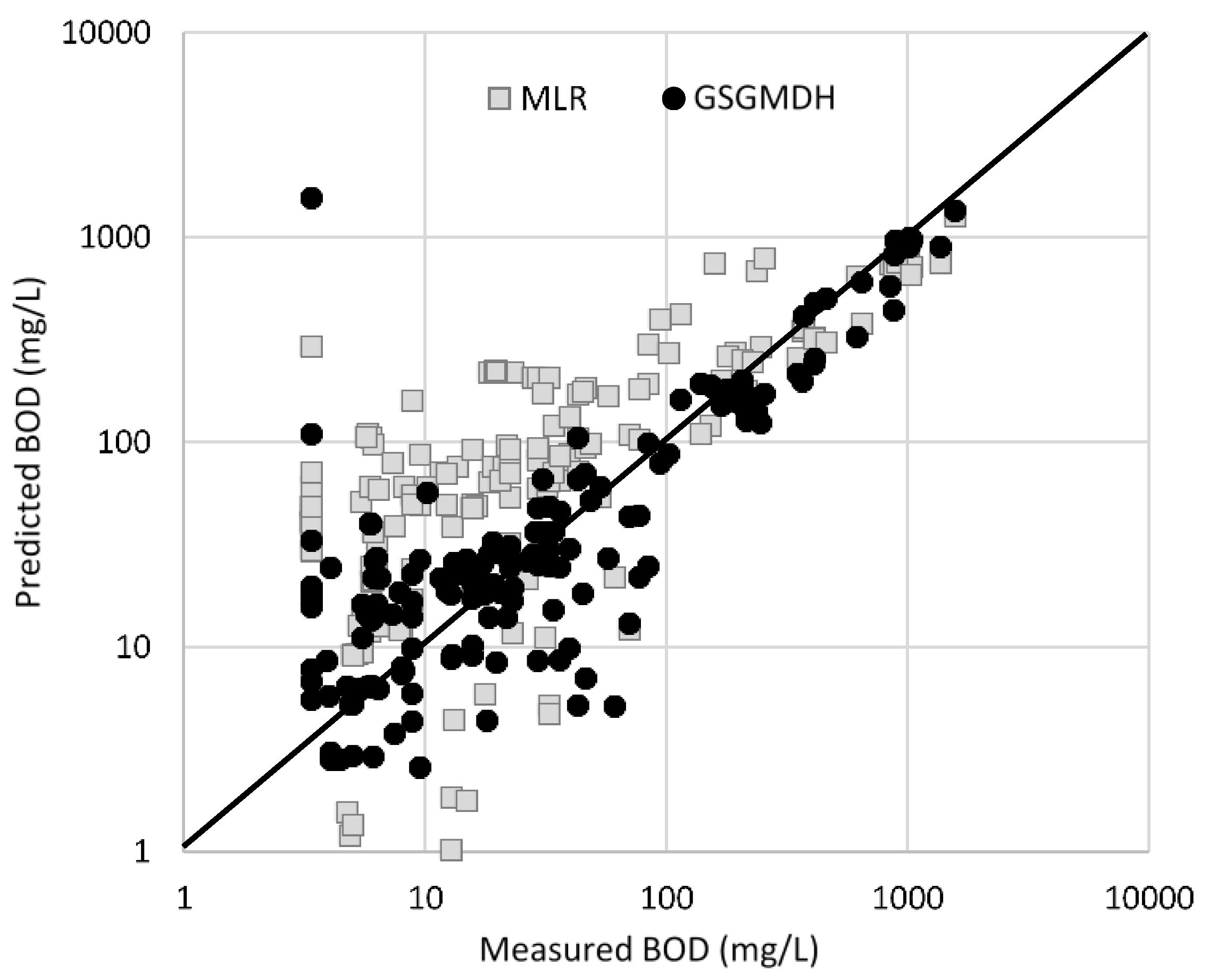
| BODTreated | GSGMDH | Train (120) | 0.99 | 36 | 106 |
| Test (52) | 0.99 | 31 | 89 | ||
| MLR | Train (120) | 0.83 | 159 | 558 | |
| Test (52) | 0.67 | 199 | 443 | ||
| CODTreated | GSGMDH | Train (123) | 0.85 | 573 | 261 |
| Test (54) | 0.91 | 619 | 192 | ||
| MLR | Train (123) | 0.54 | 890 | 820 | |
| Test (54) | 0.73 | 575 | 943 | ||
| TPTreated | GSGMDH | Train (62) | 0.73 | 8.99 | 428 |
| Test (28) | 0.91 | 5.66 | 457 | ||
| MLR | Train (62) | 0.59 | 6.40 | 58 | |
| Test (28) | 0.80 | 12.8 | 63 | ||
| TNTreated | GSGMDH | Train (57) | 0.96 | 3.49 | 310 |
| Test (29) | 0.96 | 4.08 | 127 | ||
| MLR | Train (57) | 0.58 | 7.60 | 68 | |
| Test (29) | 0.70 | 10.9 | 54 |
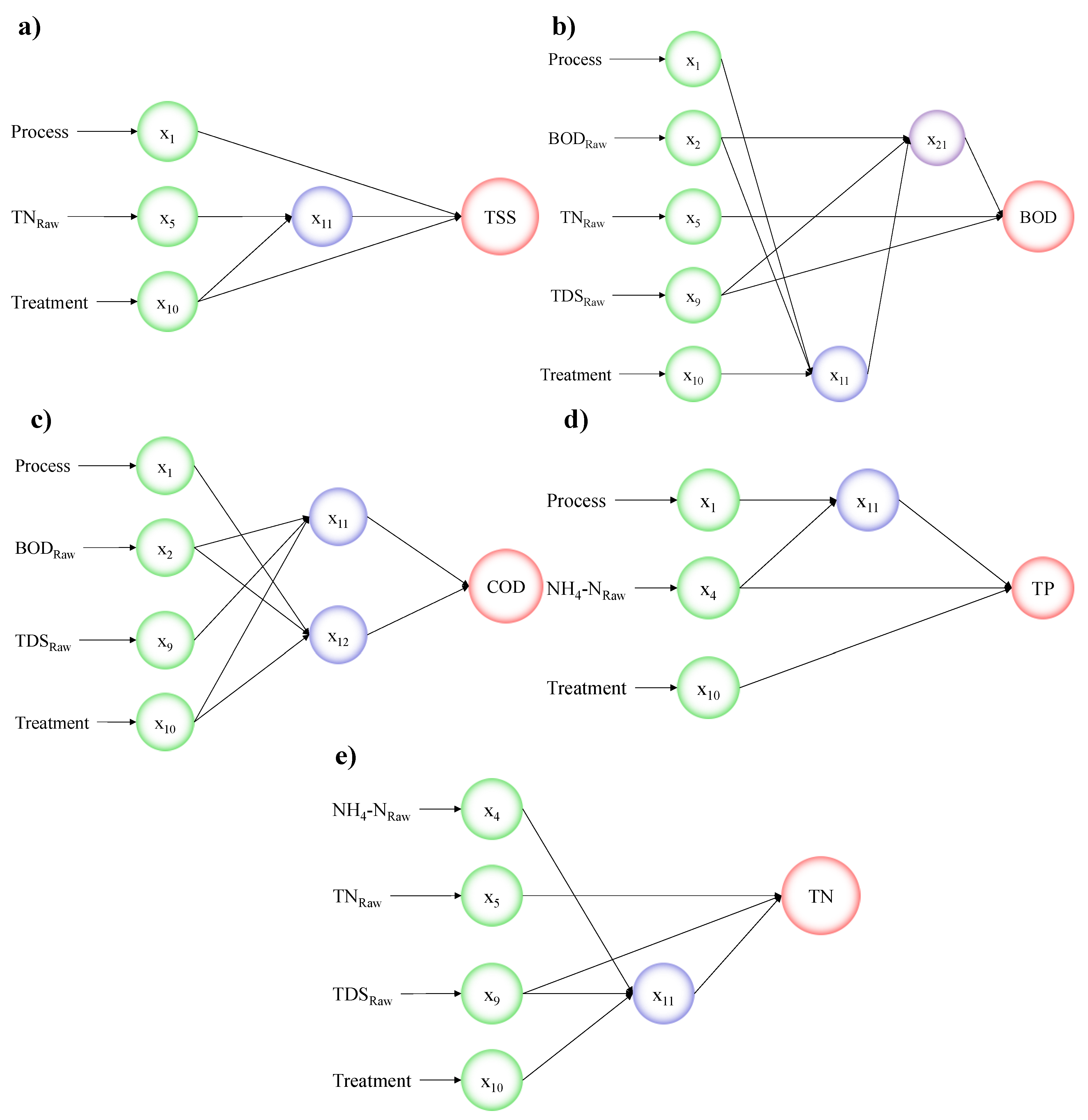
| Input Parameters for all Following Models: x1 = Process, x2 = BODRaw, x3 = CODRaw, x4 = NH4−NRaw, x5 = TNRaw, x6 = TPRaw, x7 = TSSRaw, x8 = TSRaw, x9 = TDSRaw, x10 = Treatment | |
|---|---|
| TSS | TSS = (|1.528 − 30.083 ∗ x11 − 15.482 ∗ x1 − 4.522 ∗ x10 + 35.961 ∗ x1 ∗ x11 + 53.634 ∗ x10 ∗ x11 − 2.429 ∗ x10 ∗ x1 + 58.95 ∗ x11 ∗ x11 + 45.6 ∗ x1 ∗ x1 + 6.614 ∗ x10 ∗ x10 − 1.355 ∗ x10 ∗ x1 ∗ x11 + 5.404 ∗ x1 ∗ x11 ∗ x11 − 23.609 ∗ x1 ∗ x1 ∗ x11 − 107.196 ∗ x10 ∗ x11 ∗ x11 + 1.459 ∗ x10 ∗ x1 ∗ x1 − 33.867 ∗ x10 ∗ x10 ∗ x11 + 0.353 ∗ x10 ∗ x10 ∗ x1 − 49.415 ∗ x11 ∗ x11 ∗ x11 − 30.274 ∗ x1 ∗ x1 ∗ x1 − 2.809 ∗ x10 ∗ x10 ∗ x10|) ∗ 7160 |
| Where: x11 = 0.137 − 0.639 ∗ x5 − 0.1419 ∗ x10 − 0.7245 ∗ x10 ∗ x5 + 3.46 ∗ x5 ∗ x5 − 0.0056 ∗ x10 ∗ x10 − 4.203 ∗ x10 ∗ x5 ∗ x5 + 1.914 ∗ x10 ∗ x10 ∗ x5 − 0.274 ∗ x5 ∗ x5 ∗ x5 − 0.0313 ∗ x10 ∗ x10 ∗ x10 | |
| BOD | BOD = (|0.008 + 0.841 ∗ x21 + 0.044 ∗ x9 − 0.128 ∗ x5 − 3.982 ∗ x9 ∗ x21 − 0.17 ∗ x5 ∗ x21 − 1.682 ∗ x5 ∗ x9 + 5.71 ∗ x21 ∗ x21 + 0.0196 ∗ x9 ∗ x9 + 0.943 ∗ x5 ∗ x5 + 3.0926 ∗ x5 ∗ x9 ∗ x21 − 2.853 ∗ x9 ∗ x21 ∗ x21 + 5.668 ∗ x9 ∗ x9 ∗ x21 − 2.219 ∗ x5 ∗ x21 ∗ x21 − 5.524 ∗ x5 ∗ x9 ∗ x9 − 1.328 ∗ x5 ∗ x5 ∗ x21 + 11.933 ∗ x5 ∗ x5 ∗ x9 − 6.199 ∗ x21 ∗ x21 ∗ x21 + 0.218 ∗ x9 ∗ x9 ∗ x9 − 3.512 ∗ x5 ∗ x5 ∗ x5|) ∗ 2298 + 2 |
| Where: x11 = −0.554 − 0.426 ∗ x10 + 0.42 ∗ x2 + 1.623 ∗ x1 − 1.652 ∗ x2 ∗ x10 + 0.224 ∗ x1 ∗ x10 + 1.517 ∗ x1 ∗ x2 + 0.724 ∗ x10 ∗ x10 + 1.265 ∗ x2 ∗ x2 − 0.766 ∗ x1 ∗ x1 + 1.322 ∗ x1 ∗ x2 ∗ x10 − 0.289 ∗ x2 ∗ x10 ∗ x10 + 1.185 ∗ x2 ∗ x2 ∗ x10 − 0.586 ∗ x1 ∗ x10 ∗ x10 − 1.6 ∗ x1 ∗ x2 ∗ x2 + 0.17 ∗ x1 ∗ x1 ∗ x10 − 1.447 ∗ x1 ∗ x1 ∗ x2 − 0.115 ∗ x10 ∗ x10 ∗ x10 − 0.622 ∗ x2 ∗ x2 ∗ x2 − 0.3 ∗ x1 ∗ x1 ∗ x1 | |
| and: x21 = −0.005 + 0.172 ∗ x11 + 0.071 ∗ x9 + 0.794 ∗ x2 + 7.808 ∗ x9 ∗ x11 + 25.691 ∗ x2 ∗ x11 − 3.26 ∗ x2 ∗ x9 − 21.654 ∗ x11 ∗ x11 − 0.7863662692 ∗ x9 ∗ x9 − 9.392 ∗ x2 ∗ x2 − 48.61 ∗ x2 ∗ x9 ∗ x11 + 17.523 ∗ x9 ∗ x11 ∗ x11 + 2.059 ∗ x9 ∗ x9 ∗ x11 − 17.201 ∗ x2 ∗ x11 ∗ x11 − 6.373 ∗ x2 ∗ x9 ∗ x9 − 20.94 ∗ x2 ∗ x2 ∗ x11 + 28.041 ∗ x2 ∗ x2 ∗ x9 + 43.899 ∗ x11 ∗ x11 ∗ x11 + 1.773 ∗ x9 ∗ x9 ∗ x9 + 8.693 ∗ x2 ∗ x2 ∗ x2 | |
| COD | COD = = (|0.000423 + 0.073 ∗ x12 + 0.79 ∗ x11 − 6.087 ∗ x11 ∗ x12 + 1.742 ∗ x12 ∗ x12 + 5.405 ∗ x11 ∗ x11 − 9.309 ∗ x11 ∗ x12 ∗ x12 + 30.949 ∗ x11 ∗ x11 ∗ x12 − 0.46 ∗ x12 ∗ x12 ∗ x12 − 22.407 ∗ x11 ∗ x11 ∗ x11|) ∗ 8298 + 2 |
| Where: x11 = −0.059 + 0.131 ∗ x10 + 1.3484 ∗ x9 − 0.694 ∗ x2 − 2.875 ∗ x9 ∗ x10 + 2.066 ∗ x2 ∗ x10 + 5.147 ∗ x2 ∗ x9 + 0.067 ∗ x10 ∗ x10 − 3.47 ∗ x9 ∗ x9 + 1.432 ∗ x2 ∗ x2 − 0.608 ∗ x2 ∗ x9 ∗ x10 + 1.315 ∗ x9 ∗ x10 ∗ x10 + 1.326 ∗ x9 ∗ x9 ∗ x10 − 1.818 ∗ x2 ∗ x10 ∗ x10 − 15.481 ∗ x2 ∗ x9 ∗ x9 − 0.94 ∗ x2 ∗ x2 ∗ x10 + 8.23 ∗ x2 ∗ x2 ∗ x9 − 0.104 ∗ x10 ∗ x10 ∗ x10 + 6.812 ∗ x9 ∗ x9 ∗ x9 − 3.527 ∗ x2 ∗ x2 ∗ x2 | |
| and: x12 = −1.119 − 6.106 ∗ x10 − 34.025 ∗ x2 − 5.377 ∗ x1 − 1.72 ∗ x2 ∗ x10 + 13 ∗ x1 ∗ x10 + 103.148 ∗ x1 ∗ x2 + 2.854 ∗ x10 ∗ x10 + 1.817 ∗ x2 ∗ x2 + 27.183 ∗ x1 ∗ x1 + 2.378 ∗ x1 ∗ x2 ∗ x10 − 0.7980132594 ∗ x2 ∗ x10 ∗ x10 + 0.834 ∗ x2 ∗ x2 ∗ x10 − 1.312 ∗ x1 ∗ x10 ∗ x10 − 1.213 ∗ x1 ∗ x2 ∗ x2 − 7.666 ∗ x1 ∗ x1 ∗ x10 − 69.104 ∗ x1 ∗ x1 ∗ x2 − 0.924 ∗ x10 ∗ x10 ∗ x10 − 1.167 ∗ x2 ∗ x2 ∗ x2 − 20.56 ∗ x1 ∗ x1 ∗ x1 | |
| TP | TP = (|−0.055 − 1.609 ∗ x11 + 0.619 ∗ x10 + 1.528 ∗ x4 − 10.509 ∗ x10 ∗ x11 + 26.087 ∗ x4 ∗ x11 − 1.137 ∗ x4 ∗ x10 + 51.713 ∗ x11 ∗ x11 − 0.738 ∗ x10 ∗ x10 − 16.005 ∗ x4 ∗ x4 + 37.421 ∗ x4 ∗ x10 ∗ x11 − 42.84 ∗ x10 ∗ x11 ∗ x11 + 8.358 ∗ x10 ∗ x10 ∗ x11 − 929.104 ∗ x4 ∗ x11 ∗ x11 − 0.0658 ∗ x4 ∗ x10 ∗ x10 + 473.109 ∗ x4 ∗ x4 ∗ x11 − 3.534 ∗ x4 ∗ x4 ∗ x10 + 322.282 ∗ x11 ∗ x11 ∗ x11 + 0.263 ∗ x10 ∗ x10 ∗ x10 − 39.329 ∗ x4 ∗ x4 ∗ x4|) ∗ 89.96 + 0.04 |
| where: x11 = −2.442 + 7.202 ∗ x1 + 0.533 ∗ x4 + 0.896 ∗ x4 ∗ x1 − 4.397 ∗ x1 ∗ x1 − 3.009 ∗ x4 ∗ x4 − 4.066 ∗ x4 ∗ x1 ∗ x1 + 21.622 ∗ x4 ∗ x4 ∗ x1 − 0.2734052233 ∗ x1 ∗ x1 ∗ x1 − 15.831 ∗ x4 ∗ x4 ∗ x4 | |
| TN | TN = (|0.079 − 0.157 ∗ x11 + 0.747 ∗ x5 − 1.742 ∗ x9 + 8.214 ∗ x5 ∗ x11 − 5.488 ∗ x9 ∗ x11 − 10.891 ∗ x9 ∗ x5 + 1.884 ∗ x11 ∗ x11 + 2.472 ∗ x5 ∗ x5 + 14.098 ∗ x9 ∗ x9 + 3.182 ∗ x9 ∗ x5 ∗ x11 − 4.938 ∗ x5 ∗ x11 ∗ x11 − 6.586 ∗ x5 ∗ x5 ∗ x11 − 8.161 ∗ x9 ∗ x11 ∗ x11 − 19.931 ∗ x9 ∗ x5 ∗ x5 + 7.19 ∗ x9 ∗ x9 ∗ x11 + 45.043 ∗ x9 ∗ x9 ∗ x5 + 1.522 ∗ x11 ∗ x11 ∗ x11 + 0.609 ∗ x5 ∗ x5 ∗ x5 − 22.436 ∗ x9 ∗ x9 ∗ x9|) ∗ 60.83 + 0.03 |
| Where: x11 = 0.124 + 0.296 ∗ x4 + 0.339 ∗ x9 − 0.06 ∗ x10 − 7.27 ∗ x9 ∗ x4 − 7.826 ∗ x10 ∗ x4 + 0.627 ∗ x10 ∗ x9 + 42.361 ∗ x4 ∗ x4 − 1.624 ∗ x9 ∗ x9 − 0.143 ∗ x10 ∗ x10 + 18.159 ∗ x10 ∗ x9 ∗ x4 − 196.991 ∗ x9 ∗ x4 ∗ x4 + 71.295 ∗ x9 ∗ x9 ∗ x4 + 0.209 ∗ x10 ∗ x4 ∗ x4 + 0.382 ∗ x10 ∗ x9 ∗ x9 + 1.765 ∗ x10 ∗ x10 ∗ x4 − 1.498 ∗ x10 ∗ x10 ∗ x9 − 2.397 ∗ x4 ∗ x4 ∗ x4 + 0.785 ∗ x9 ∗ x9 ∗ x9 + 0.258 ∗ x10 ∗ x10 ∗ x10 |
Publisher’s Note: MDPI stays neutral with regard to jurisdictional claims in published maps and institutional affiliations. |
© 2021 by the authors. Licensee MDPI, Basel, Switzerland. This article is an open access article distributed under the terms and conditions of the Creative Commons Attribution (CC BY) license (https://creativecommons.org/licenses/by/4.0/).
Share and Cite
Mundi, G.; Zytner, R.G.; Warriner, K.; Bonakdari, H.; Gharabaghi, B. Machine Learning Models for Predicting Water Quality of Treated Fruit and Vegetable Wastewater. Water 2021, 13, 2485. https://doi.org/10.3390/w13182485
Mundi G, Zytner RG, Warriner K, Bonakdari H, Gharabaghi B. Machine Learning Models for Predicting Water Quality of Treated Fruit and Vegetable Wastewater. Water. 2021; 13(18):2485. https://doi.org/10.3390/w13182485
Chicago/Turabian StyleMundi, Gurvinder, Richard G. Zytner, Keith Warriner, Hossein Bonakdari, and Bahram Gharabaghi. 2021. "Machine Learning Models for Predicting Water Quality of Treated Fruit and Vegetable Wastewater" Water 13, no. 18: 2485. https://doi.org/10.3390/w13182485
APA StyleMundi, G., Zytner, R. G., Warriner, K., Bonakdari, H., & Gharabaghi, B. (2021). Machine Learning Models for Predicting Water Quality of Treated Fruit and Vegetable Wastewater. Water, 13(18), 2485. https://doi.org/10.3390/w13182485