Abstract
Designing a small hydropower plant (SHPP) necessitates fulfillment of energy and ecological constraints, so a well-defined design flow is of the utmost significance. The main parameters of each SHPP are determined by appropriate techno-economic studies, whereas an improved approach to defining more precise SHPP installed parameter is presented in this paper. The SHPP installed parameter is the ratio of the design flow and averaged perennial flow obtained from the flow duration curve at the planned water intake location. Previous experiences in the design of SHPPs have shown that the SHPP installed parameter has a value in a wide range without the existence of an unambiguous equation for its determination. Therefore, with this aim, the thirty-eight (38) small watercources in the territory of Montenegro, denominated for the construction of SHPPs, have been investigated. SHPPs are divided into two groups depending on the installed capacity and the method of calculating the purchase price of electricity. For both groups, the range of SHPP installed parameter is determined according to the technical and economic criteria: the highest electricity production, the highest income, net present value (NPV), internal rate of return (IRR), and payback period (PB).
1. Introduction
The generated power from large and small hydropower plants remains a significant source of renewable energy. Worldwide installed capacity of hydropower reached 1308 GW with 4306 TWh of produced energy in 2019 [1]. In 2018, global electricity generation from all renewables was about 25.6%, while hydropower produced 15.9% on the global level [2], meaning that hydropower made up 62.1% of all renewable electricity generation. The small hydropower plant (SHPP) with installed capacity up to 10 MW is one of the most cost-effective energy technologies on a small scale due to its predictable energy characteristics, long term reliability, and reduced environmental effects [3]. The levelized cost of electricity (LCOE) of SHPPs is a bit higher than LCOE of large hydropower plants, and it is in a range from 11 to 13 cEUR/kWh [4]. The majority of SHPPs are of the run-off river (RoR) type, which is different in design, appearance, and impact compared to large hydro power plants. Generating energy at RoR plants is proportional to water inflow, and there is a little variation in electrical output during the day. These type of plants are designed for a large flow rate with a small head on large rivers with gentle gradients, or a small flow rate with a high head on small rivers with steep gradients [5]. Optimum infrastructure size and design should provide optimum net present value (NPV), taking into consideration the hydrology conditions and tariff of electric energy during the lifetime of the SHPP project [6]. The choice of optimum SHPP design is a fundamental goal for maximizing both the cost effectiveness of the investment and the hydro energy utilization of water resources [7,8]. The amount of energy generated during the year is the most important issue worthy of study in the RoR SHPP studies. Therefore, determining the optimal design flow is one of the most important factors in planning SHPPs [9]. To date, there is no unambiguous equation for its determination. Najmaii and Movaghar [10] developed a mathematical model able to determine optimal flow for a proposed set of the turbines as well as maximum power and energy output and the maximum net yearly benefit. Eliasson et al. [11] developed genetic algorithm method used as a computer model to find the global optimization of design and layout of hydropower projects by maximizing the net profit of the investment. Voros et al. [12] introduced an empirical short-cut design method for selection of the nominal turbine flow rate in terms of maximizing the economic benefits of the investments. Karlis and Papadopoulos [13] developed a software for the systematic assessment of the technical feasibility and economic viability of SHPPs. They pointed out that NPV and internal rate of return (IRR) are, among the other economic factors, the most used in the field of the hydro power. Paish [14] summarized the main advantages and shortcomings of SHPPs, new technology innovations that have been developed, and the barriers for further development. He stressed that small hydropower is accepted as a renewable energy source, easy to develop and with a small impact on the environment. Montanari [15] presented an original method based on the use of NPV which is calculated using design flow, net head, and hydrology characteristics from the location investigated. Kaldellis et al. [16] presented the study on the systematic investigation of the techno-economic viability of SHPPs. It was shown that the IRR value of SHPP installation is higher than 18% for most cases, and that the IRR value reaches its maximum after 10 to 15 years of plant operation. Andaroodi [17] developed software which helps in the selection of the optimum design flow for a certain head with compromise and judgment through the economic parameters. Forouzbakhsh et al. [18] concluded that Build Operate and Transfer (BOT) contract is a favourable way to develop SHPP projects with improved NPV and other economic indices, compared to the contracts with less inclusion of the private sector. Anagnostopoulos, D.E. Papantonis [19] found that the NPV, as well as annual electricity production, constitutes two principal objectives, whose maximization can lead to the most advantageous design. Varun et al. [20] showed that the energy payback period for RoR SHPPs decreases with increase in the plant’s installed capacity. Bockman et al. [21] presented a real options-based method for making the optimal investment decision in the field of small hydro power in a power market with uncertain prices. Alexander and Giddens [22] proposed an equation for calculating the optimum flow rate for any given diameter of the pipeline, but valid only in cases in which pipeline energy losses are one third of the gross head. Peńa et al. [23] developed a procedure for estimating the water flow of a water intake location, based on the time series forecasting methods, and used an obtained flow duration curve to determine the turbine design flow. Ogayar and Vidal [24] developed a set of equations, based on the net head and installed capacity, for determining the cost of the electromechanical equipment for SHPPs. Aggidis et al. [25] developed the empirical equations for determining minimum costs of potential sites for SHPPs, the cost of energy production as well as cost of electromechanical equipment with different types of hydraulic turbines. Mishra et al. [26] developed correlation for the cost of electro-mechanical equipment and showed that an increase in the net head is followed by the decrease in this cost. Santolin et al. [27] took into consideration seven technical and economical parameters, the annual energy production, NPV, and IRR, among the others, in order to calculate the proper capacity sizing of SHPP. They concluded that simultaneous analysis of technical and economic aspects can lead to optimum design based on the desired performance, profitability, and feasibility of the plant. Mishra et al. [28] concluded that, usually, the net head and installed capacity are used as cost-influencing parameters for cost determination of SHPPs, and advised that more parameters, such as flow, turbine speed, runner diameter, and setting of the turbine, should be used for improving cost correlations. Basso and Botter [29] developed an analytical model that contains a set of analytical expressions for the design flow, which maximizes generated energy and profitability of an RoR plant. Barelli et al. [30] proposed a design approach for SHPPs based on a recalculated flow duration curve. The approach was applied on three torrential rivers in Italy, and the authors found the optimum design flow for the cases investigated. Carapellucci et al. [31] defined methodology for evaluating technical and economic potential of SHPPs. The proposed energy model evaluates the main technical parameters of potential SHPP, while the economic model is able to estimate the profitability of the initial investment by determining profitability index and discounted payback period. Nicotra et al. [32] proposed a simple method for evaluating the technical (installed capacity) and economic (costs and incomes) feasibility of micro hydro power plants in existing irrigation systems. Tiago Filho et al. [33] presented aspect factor (AF), as a function of capacity and head, used to estimate the cost of the SHPPs. More recently, Mamo et al. [34] presented mathematical model which gives the optimum design flow, number of the turbines and installed capacity of RoR plants. Hounnou et al. [35] proposed a multi-objective optimization procedure for the optimal sizing of RoR small hydropower plants, considering annual generated energy and investment cost simultaneously. Yildiz and Vrugt [36] developed software which simulates technical and economic parameters of RoR and helps users to choose their optimal design.
Montenegro belongs to a small group of European countries in which water is the most important natural resource. This is evidenced by the fact that average annual rainfall is 1138 mm/m2, which is one of the highest values in Europe. Due to the topographical characteristics of the terrain, intertwined with watercourses, Montenegro’s theoretical hydro potential is rated to 9.8 TWh annually [37]. As Montenegro is classified as one of the European countries with a very rich water potential, it is indisputable that the government must use this potential as the strongest benefit for economic and social development. With adoption of the Energy Law in 2003, as well as the signing of the Agreement on the formation of the Energy Community in 2005, the transformation of the energy sector in Montenegro began [38]. The process of the new SHPPs development campaign in Montenegro began with the adoption of the Small Hydropower Development Strategy in 2006 [39]. During 2010 and 2011, flow on 65 small watercourses was measured under the project named the Registry of Small Rivers and Potential Locations of SHPPs at Municipality Level for Central and Northern Montenegro, and relevant flow duration curves (FDCs) were obtained [40]. This Registry was enhanced during 2018 and 2019 [41]. The Energy Development Strategy of Montenegro until 2030 [42], as well as the National Action Plan for Renewable Energy Sources by 2020 [43], are the planning dynamics of the development of SHPPs.
Locations for SHPPs in Montenegro are characterized by relatively low average annual flows and high gross heads. Some of the proposed sites for building SHPPs are shown on Figure 1.
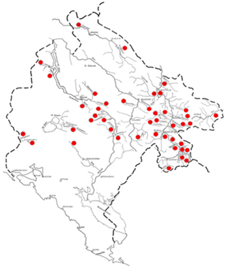
Figure 1.
Locations where SHPPs are envisaged [39].
Since 2013, 15 new SHPPs have been finished and put into operation, with a total installed capacity of 25 MW and annual electricity production of 80.2 GWh.
Small rivers in Montenegro, envisaged for hydro energy utilization, are mostly insufficiently studied mountain watercourses. Due to the fact that design flow is one of the most important parameters during SHPP planning, methodology is developed in order to determine more precise SHPP installed parameter. This paper aims to narrow down a range for SHPP installed parameters in RoR plants for the case of mountain torrential rivers, taking into consideration technical (the highest annual generated electricity) and economical (the highest annual income, NPV, IRR, and payback period) criteria. After examining all the investigated parameters, the range of SHPP installed parameters is narrowed, with clear recommendations for investors and developers of SHPPs, applicable to the sites with high gross heads, low average annual flows, and sharp flow duration curves. The novelty of this work is also in finding and improving access and a unique installed parameter that will unify the solution, properly classify watercourses, and serve for quality selection of suitable types of hydro units, thus confirming the appropriate techno-economic analysis and respecting legal regulations and environmental standards.
2. Materials and Methods
In this paper, 38 (thirty-eight) small watercourses in the territory of Montenegro, on which construction of small hydropower plants with different capacities are planned or have already been designed, have been investigated. Twelve (12) locations have been already built, six (6) of them are under construction, and twenty (20) locations are planned to be constructed and are in different stages of the projects. In order to obtain experimental hydrological data for small watercourses in Montenegro, very detailed measurements were made within the period of two years. Prior to the measurements, it was necessary to clearly define the locations where the measurements would be performed, as well as the permanent flow measurements procedures, in order to obtain relevant data for the necessary analyses. Hydrology data (flow duration curve with determined averaged perennial flow) for each watercourse are known [40,41,44]. Firstly, average annual flow is determined as a sum of the average daily flows divided by the number of days according to following equation,
where QavA is the average annual flow, QavD is the average daily flow, and ND is the number of days in one year. Secondly, average perennial flow is determined as the arithmetic mean of the average annual flows available for a given period,
where Qav is the average perennial flow and Ny is the the number of years.
Based on hydrology data, the ecological flow is determined, i.e., the minimum amount of water that must remain in the watercourse in order to preserve the natural balance of aquatic ecosystems and ecosystems related to water [45]. The position of the water intake and power house is mostly determined on the basis of topographic maps, orientation route of the pipeline [46], and data from the above mentioned Registry.
The SHPP installed parameter is defined as the ratio of the design flow and averaged perennial flow according to the following equation,
It is assumed that Ki for each watercourse initially ranges from 1.0 to 2.5 [47]. In addition to hydrological data, the collection and unification of suitable types of hydraulic turbines from well-known world manufacturers was carried out, considering and adapting their energy characteristics to the diversity and specifics of mountain rivers. For the obtained values of design flow, a net head, pipeline diameter, installed capacity, and annual electricity production were calculated for the chosen type of the turbine [48]. This procedure gives 16 variants for each watercourse with Ki step of ΔKi = 0.1 or 608 alternatives of observed parameters (capacity, annual electricity production, income, NPV, IRR, and PB) in total. The analysis of economic parameters was based on regionally current prices, as well as for the European small hydropower market. Then, appropriate mathematical models were made, and in-house software was developed [49,50]. For any value of design flow, the software makes an optimization procedure whose output are net head and diameter of the pipeline. Based on these calculations, the design flow which gives both the highest electricity production, the highest gross income and the best economic parameters has been determined. Administrative provisions often impose external constraints on the design, which may lead to deviations from the optimum sizing of the plant [51]. Such administrative impacts are beyond the scope of the present paper.
The effective capacity at the plant’s threshold is the power that is obtained when taking into account losses in the turbine, generator, and transformer [8],
where Ph is the hydraulic power, ρ is the mass density, g is the gravitational acceleration, Qd is the design flow, Hn is the net head, ηt is the turbine efficiency, ηg is the generator efficiency, and ηtr is the transformer efficiency. According to the rules for calculating the purchase price of energy from the SHPPs [52], the incentive energy prices are determined depending on the capacity at the plant’s threshold in the manner defined in Table 1. It should be noted that SHPPs with capacity below 1 MW and above 8 MW have a constant values of incentive price.

Table 1.
Electricity prices depending on the capacity of the power plant [52].
With the increase in capacity on the threshold of the power plant, the incentive price decreases from the maximum value of 10.44 cEUR/kWh for power plants with capacity less than 1 MW to the value of 6.8 cEUR/kWh for power plants with capacity larger than 8 MW. The total decrease in the incentive price with an increase in capacity at the power plant threshold is about 35%. By varying the design flow Qd = Ki·Qav = (1.0 ÷ 2.5)·Qav, capacity, annual energy production, gross income, NPV, IRR, and PB are calculated for every design flow, where Qav is averaged perennial flow. Annual energy production is calculated with flow that changes according to FDC, taking into account decreasing turbine efficiency with decreasing flow through the turbine, as well as ecological flow and cut-off flow of the chosen turbine. Cut-off flow or technical minimum of the turbine is the minimum flow rate on which turbine is able to work with sufficient efficiency. Pelton, Cross-flow, and Francis turbines are used as a solution for hydro energy utilization for all rivers with cut-off flow of Qcut-off = {0.1Qd; 0.1Qd; 0.3Qd}, respectively [53]. The annual gross income of the small power plant is calculated from the generated energy and the incentive energy prices. Based on this approach, investigated rivers can be divided into two groups according to the capacity range (Table 2).
Table 2.
River groups based on capacity range.
The capacity range means that all calculated plant capacities obtained for all different values of Ki with a step of 0.1 belong to the proposed range. Group I fits with the range of the incentive price, but this is not the case with Group II, which intersects between different ranges of the incentive price. Group I has 16 SHPPs and Group II has 22 SHPPs. Finally, the initial range of SHPP installed parameter is narrowed for both groups of rivers.
The net present value (NPV) is defined as the value of the net cash flow during exploitation period of SHPP discounted back to its present value and it is calculated according to the next equation [27,29],
where R is the annual net income of the SHPP, C is the annual costs of the SHPP (in the first year this is total investment costs of the project and in the all next years this is the operation and maintenance costs), d is the discount rate (d = 8% for Montenegro), and T is the time of cash flow, equal to concession period of 30 years. The total investment costs of the plant are computed as the sum of the cost of the different parts and components, i.e., civil works including penstock, electro-mechanical, and hydro-mechanical equipment, connection to the electrical network, project design, and supervision. Investment assessment for individual parts and components is formed on the basis of Montenegrin experience, except for the cost of electro-mechanical equipment. In this case, Montenegrin experience is coupled with several references [16,24,25,26,27,28,31,33] and more than 100 collected offers, available to the authors of the paper, for electro-mechanical equipment for SHPPs in Montenegro. The operation and maintenance costs can be divided into the fixed and the variable costs. The fixed costs can include employee salaries, administrative costs, property benefits, insurance costs, etc. The group of variable costs includes the concession fee, interest expense on loans, and the fee for the license for the production of electricity, as well as costs of regular overhaul and maintenance of the equipment.
The internal rate of return (IRR) is the discount rate that reduces the present value of the net project cash flow to zero in a discounted cash flow analysis and can be calculated from Equation (3), as the value of d corresponding to a NPV = 0, [27,29].
The payback period (PB) is the period of time it takes to recover the cost of an investment and it is obtained dividing total investment costs with net annual income of SHPP.
3. Results
The first group (Group I) are plants with installed capacity below 1 MW and basic parameters are shown in Table 3 and Table 4. Table 3 shows maximum annual electricity production, income and finally corresponding SHPP installed parameter. Table 4 shows the economic parameters IRR, NPV, and PB and the corresponding obtained values for Ki. It can be observed that for all 16 watercourses the value of Ki = 2.5 gives the maximum annual electricity production and the maximum income. This is not the case for NPV and IRR. Some watercourses give the value Ki = 2.5, but most offer different ones. In some cases, the same value for Ki is obtained for NPV and IRR, while in some, different values are obtained. Therefore, it can be noticed that if the annual production and annual income are considered as a decision parameter, a practically unambiguous value of Ki = 2.5 is obtained for the considered group of power plants below 1 MW. The situation is completely different if economic parameters are considered as decision criteria. The SHPP installed parameter for the maximum value of NPV is in the range of Ki = (1.3 ÷ 2.5) where only one watercourse has Ki = 1.3, and if it was excluded from consideration then the range of the SHPP installed parameter would further be narrowed to Ki = (1.6 ÷ 2.5). If the IRR is observed, then the SHPP installed parameter is in the range of Ki = (1.6 ÷ 2.5). Thus, the economic parameters of NPV and IRR for a group of power plants with an installed capacity below 1 MW give, it can be said, the same range of the SHPP installed parameter. Payback period corresponds to maximum value of IRR and its range is very wide, i.e., PB = (5.4 ÷ 16.0) years. For Group I, the range of Ki is narrowed from initially Ki = (1.0 ÷ 2.5) to Ki = (1.6 ÷ 2.5) Maximum IRR and NPV is obtained for the Umski SHPP, and they are IRR = 18.94% and NPV = 1466.40 kEUR.
Table 3.
Maximum annual production and income and corresponding SHPP installed parameter for SHPPs below 1 MW—Group I, (*—constructed plants).
Table 4.
Internal rate of return, net present value, payback period, and corresponding SHPP installed parameter for SHPPs below 1 MW—Group I.
Next three characteristic examples from Group I are considered: Hridska SHPP, which has the same value of the SHPP installed parameter for all considered parameters; Jasičje SHPP, where the SHPP installed parameter is the same for NPV and IRR; and Bukovičko SHPP, where all three values of the SHPP installed parameter are different (Table 5).
Table 5.
Typical examples for Group I.
Hridska SHPP has the Ki = 2.5 obtained from all parameters, which means that for this plant’s maximum value of Ki gives the best performance regarding both the technical and economical view. Hridska SHPP started with a capacity of 412.8 kW for Ki = 1.0 and finished with 999.8 kW for Ki = 2.5 having, for all capacities, a constant incentive price (Table 1). Due to this fact, annual electricity production and annual income exhibit permanent and similar rising behavior (Figure 2a). Figure 2b shows the change in NPV, IRR, and PB as a function of Ki. NPV and IRR continuously increase from minimum to maximum value, with NPV having a slightly sharper growth. On the other hand, as expected, PB decreases with the increase in these parameters. The total investment is 1.37 mEUR, and the payback period is PB = 8.7 years.
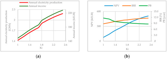
Figure 2.
(a) Annual electricity production and income—Hridska SHPP; (b) NPV, IRR, and PB—Hridska SHPP.
The increase in capacity and production at Ki = 1.8 is due to the increase in pipeline diameter from DN500 to DN600. With Hridska SHPP, there is no doubt that the value Ki = 2.5 is chosen for the SHPP installed parameter.
Figure 3 shows the change in annual electricity production, income, NPV, IRR, and PB, as a function of Ki for Jasičje SHPP. The maximum value of annual production and income was obtained for Ki = 2.5 (Figure 3a). This SHPP started with capacity of 323.8 kW for Ki = 1.0 and finished with capacity of 807.2 kW for Ki = 2.5. The total investment for this value of Ki is 1.65 mEUR. Maximum values of NPV (657 kEUR) and IRR (12.34%) are obtained for the same value of the SHPP installed parameter, Ki = 1.9 (Figure 3b). The total investment in this case is 1.46 mEUR and the payback period is 8.2 years. For Ki = 2.0, the diameter increases from DN600 to DN700, which leads to an increase in investment and a decrease in the economic parameters of NPV and IRR. On the other hand, this increase in diameter leads to an increase in annual electricity production and annual income. The difference in annual income obtained for Ki = 2.5 and Ki = 1.9 is around 13 kEUR, and difference in total investment is 190 kEUR. It is obvious here that the value of SHPP installed parameter Ki = 1.9 should be chosen as the best choice for the case investigated.
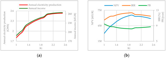
Figure 3.
(a) Annual electricity production and income—Jasičje SHPP; (b) NPV, IRR, and PB—Jasičje SHPP.
Figure 4 shows electricity production, income, NPV, IRR, and PB in function of Ki for Bukovičko SHPP. This SHPP started with capacity of 285.8 kW for Ki = 1.0 and finished with 716.1 kW for Ki = 2.5. The annual electricity production and income permanently rise up to Ki = 2.5 with a total investment of 1.36 mEUR and a payback period of 9.66 years. On the other hand, maximum values of NPV (378.2 kEUR) and IRR (11.3%) are obtained for Ki = 1.8 and Ki = 1.6, respectively (Figure 4b). Total investment for maximum NPV is 1.15 mEUR and 1.10 mEUR for maximum IRR, and corresponding payback periods are 8.94 and 8.89 years, respectively. The difference in income is 14.3 kEUR compared with income obtained for maximum NPV, and 20.7 kEUR compared with income obtained for maximum IRR. The difference in investment between highest income and maximum NPV is 210 kEUR and between highest income and maximum IRR is 260 kEUR. The difference in investment is more than ten times higher than difference in income, which means that SHPP installed parameters obtained for maximum NPV and IRR are more preferable as optimal solution for Bukovičko SHPP. Keeping in mind that SHPP installed parameter obtained for maximum IRR gives the lower investment and payback period, compared to SHPP installed parameter obtained for maximum NPV, the self-imposed conclusion is that in this particular case the optimal value of SHPP installed parameter is Ki = 1.6.
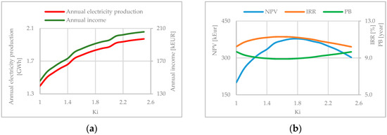
Figure 4.
(a) Annual electricity production and income—Bukovičko SHPP; (b) NPV, IRR, and PB—Bukovičko SHPP.
The second group (Group II) are plants whose installed capacity range starts from 0.4 MW and finish with 2.4 MW. Table 6 shows maximum annual electricity production and income and finally corresponding SHPP installed parameters. Table 7 shows the economic parameters IRR, NPV, and PB and the corresponding obtained values for Ki. SHPP installed parameter, which for each considered case gives the maximum annual electricity production, has the value Ki = 2.5. Therefore, if maximum annual electricity production was the only parameter under consideration, the maximum value of Ki would always be chosen. If the maximum annual income is observed, then the value of the SHPP installed parameter ranges from Ki = {1.5 ÷ 2.5}, where only three SHPP Ki < 2.0. For the 19 considered SHPPs belonging to the Group II, range of SHPP installed parameter is Ki = {2.0 ÷ 2.5}. It is obvious that higher values of SHPP installed parameters give a higher annual revenue. The situation is quite different when it comes to IRR and NPV for Group II. For both parameters, the range Ki is narrowed, but from the upper limit, and is Ki = {1.0 ÷ 2.1} which can be seen from Table 7. This appears due to the specific price policy in Montenegro, which decreases the incentive price when an SHPP installed capacity becomes higher than 1MW (Table 1). The payback period is also wide, and ranges from 4.3 years for the Trnovačka SHPP to 13.5 years for the Bukovica 1 SHPP. Maximum IRR and NPV is obtained for Trnovačka SHPP and they are IRR = 24.45% and NPV = 2892.4 kEUR.
Table 6.
Maximum annual production and income and corresponding SHPP installed parameter for SHPPs from 0.4 MW to 2.4 MW—Group II, (*—constructed plants).
Table 7.
Internal rate of return, net present value, payback period, and corresponding SHPP installed parameter for SHPPs from 0.4 MW to 2.4 MW—Group II.
Furthermore, four characteristic examples from Group II are considered; Kaludarska SHPP, which has the same value of the SHPP installed parameter for annual income, IRR, and NPV (Ki = 1.5) and the maximum for annual electricity production (Ki = 2.5); Bistrica Lipovska SHPP, where the SHPP installed parameter is the same for electricity production and income (Ki = 2.5), as well as for IRR and NPV (Ki = 1.3); Vrelo SHPP where the values of the SHPP installed parameter are the same for income and NPV (Ki = 1.9) and different for production (Ki = 2.5) and IRR (Ki = 1.6); and Stožernica SHPP where different values of Ki are obtained for all considered parameters (Table 8).
Table 8.
Typical examples for Group II.
Figure 5a shows annual electricity production and income and Figure 5b depicts NPV, IRR, and PB for Kaludarska SHPP in function of Ki.
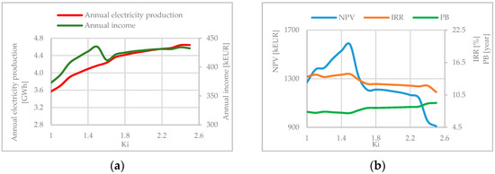
Figure 5.
(a) Annual electricity production and income—Kaludarska SHPP; (b) NPV, IRR, and PB—Kaludarska SHPP.
Kaludarska SHPP started with the capacity of 641.0 kW for Ki = 1.0 and finished with 1606.0 kW for Ki = 2.5. The annual electricity production permanently rises up to Ki = 2.5 with maximum value of 4.643 GWh/year, but it should be noted that annual electricity production is practically the same for Ki = 2.4 and equal to 4.641 GWh/year. The maximum value of annual income is obtained for Ki = 1.5 (Figure 5a), as for this value of SHPP, the installed capacity is below 1 MW (956.4 kW), and for the next value of Ki = 1.6, the installed capacity is 1012.4 kW, which imposes a decrease in incentive price according to Table 1, and an according drop in annual income. Increase in pipeline diameter from DN800 to DN900 for Ki = 1.7 recovers annual income, which rises after that, but not enough to achieve the value obtained for Ki = 1.5. The maximum values of NPV (1580.9 kEUR) and IRR (14.37%) are obtained also for Ki = 1.5 (Figure 5b). Total investment is 2.35 mEUR with the payback period of 7.2 years. There is no doubt that Ki = 1.5 is the optimal solution for Kaludarska SHPP.
Annual electricity production and annual income for Bistrica Lipovska SHPP are shown on Figure 6a, and their economic parameters NPV, IRR, and PB are depicted on Figure 6b. Bistrica Lipovska SHPP started with a capacity of 760.0 kW for Ki = 1.0 and finished with 1890.0 kW for Ki = 2.5. From Figure 6a, it can be seen that the transition from one equation for calculating the incentive price to another occurs for Ki = 1.4, when changing installed capacity from 986 kW for Ki = 1.3 to 1052 kW for Ki = 1.4. Due to that, the annual income decreases from 457.3 kEUR for Ki = 1.3 to 437.5 kEUR for Ki = 1.4. Unlike the previously considered case (Kaludarska SHPP), Bistrica Lipovska SHPP has a rapid recovery of annual income for Ki = 1.5, due to the transition from pipeline diameter from DN1100 to DN1200, and its further growth up to a maximum value of 496.7 kEUR for Ki = 2.5.
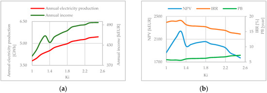
Figure 6.
(a) Annual electricity production and income—Bistrica Lipovska SHPP; (b) NPV, IRR, and PB—Bistrica Lipovska SHPP.
When it comes to economic parameters for Bistrica Lipovska SHPP, the situation is as follows. The maximum value of NPV and IRR was obtained for Ki = 1.3, namely NPV = 2237.1 kEUR and IRR = 18.65%. Payback period that corresponds to maximum IRR is PB = 5.6 years. Total investment for Ki = 1.3 is 1.91 mEUR and total investment for Ki = 2.5 is 2.71 mEUR, with difference in investment of 800 kEUR. The difference in annual income between Ki = 2.5 and Ki = 1.3 is 39.4 kEUR, which means that the invested funds are 20.3 times higher than the income that can be realized if Ki = 2.5 is chosen as the optimal value. In this particular case of Bistrica Lipovska SHPP, it is obvious that the optimal value of SHPP installed parameter is Ki = 1.3.
Figure 7 shows the main parameters for Vrelo SHPP. This plant started with capacity of 516.5 kW for Ki = 1.0 and finished with 1268.1 kW for Ki = 2.5. As in all previous cases, maximum annual electricity production is obtained for Ki = 2.5. Annual income has similar behavior as for Kaludarska SHPP; it has maximum for Ki = 1.9, and after that has sharp drop for Ki = 2.0 due to crossing the border of 1 MW of plant installed capacity. Maximum NPV = 2069.6 kEUR is also obtained for Ki = 1.9, and for this plant NPV and annual income give the same optimal value of SHPP installed parameter. On the other hand, maximum IRR = 20.93% is obtained for Ki = 1.6, but with a very close value of 20.11% for Ki = 1.9. Payback period is 4.97 years for Ki = 1.6 and 5.17 years for Ki = 1.9. Consequently, it could be concluded that Ki = 1.9 is the optimal value for Vrelo SHPP.
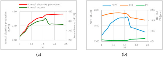
Figure 7.
(a) Annual electricity production and income—Vrelo SHPP; (b) NPV, IRR, and PB—Vrelo SHPP.
Finally, parameters for Stožernica SHPP are shown in Figure 8. This plant started with a capacity of 678.8 kW for Ki = 1.0 and finished with 1667.5 kW for Ki = 2.5. The maximum annual electricity production is obtained for Ki = 2.5, while annual income has one extreme for Ki = 1.4 (capacity 944.8 kW), dropping after that for Ki = 1.5 (capacity 1004.5 kW), due to crossing the border of 1 MW, and finally rising with practically constant value of around 447 kEUR for Ki = (2.2 ÷ 2.5). A maximum value of 447.7 kEUR is obtained for Ki = 2.3. This annual income is higher than income obtained for Ki = 1.4 for 7.4 kEUR, and the difference in investment for Ki = 2.3 and Ki = 1.4 is 560 kEUR. It is clear that Ki = 1.4 is more favorable as an optimal solution. This is confirmed in Figure 8b. A maximum value of NPV = 2055.5 kEUR is also obtained for Ki = 1.4, with a permanent drop after this value of SHPP installed parameter. IRR has maximum value of 18.07% for Ki = 1.2, but is very close to the value obtained for Ki = 1.4, which is 17.77%. There is no doubt that the optimal solution for Stožernica SHPP is Ki = 1.4.
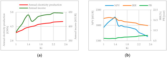
Figure 8.
(a) Annual electricity production and income—Stožernica SHPP; (b) NPV, IRR, and PB—Stožernica SHPP.
4. Conclusions
The determination of SHPP installed parameter is one of the main goals during the design of small hydro power plants. Previous experience shows that the range of SHPP installed parameter is very wide. Therefore, there is a need to determine the SHPP installed parameter in a more precise and improved way. The main intention of this paper is to narrow down the range of SHPP installed parameter for the cases of mountain torrential watercourses using techno-economic parameters. Thirty-eight small watercourses from the territory of Montenegro, on which SHPPs are planned or have already been designed, are investigated. The rivers were divided into two groups, one for which plant capacity always stays below 1 MW (Group I, with 16 plants) and a second for which plant capacity started below 1 MW and finished above 1 MW (Group II, with 22 plants). Based on the available hydrology data, an initial range of Ki = (1.0 ÷ 2.5) is adopted and for each value, with step of ΔKi = 0.1, the main techno-economic parameters of every plant are calculated with 608 alternatives in total. According to these parameters, optimal and more accurate values of SHPP installed parameters are defined by narrowing its range.
Considering the obtained results, the following conclusions can be drawn:
Group I
- 1.
- Annual electricity production and annual income give the highest examined value of Ki = 2.5 as the optimal solution for all considered plants.
- 2.
- The economic parameters NPV and IRR narrowed the initial value of SHPP installed parameter range to Ki = (1.6 ÷ 2.5).
- 3.
- By studying a few typical examples, it can be noticed that NPV and IRR have more influence on the choice of SHPP installed parameter compared to annual electricity production and income.
Group II
- 4.
- Annual electricity production for any case gives chosen upper limit of Ki = 2.5 as the optimal solution.
- 5.
- The highest annual income gives the range of SHPP installed parameter range of Ki = (2.0 ÷ 2.5).
- 6.
- NPV and IRR also narrow the range of the Ki, but from the upper limit, and for this group of plants it is Ki = (1.0 ÷ 2.1).
- 7.
- Examination of several typical examples shows that NPV and IRR are more influential parameters for choosing Ki compared to annual electricity production and income.
- 8.
- Due to higher and constant incentive price, the SHPP installed parameter which gives capacity below 1 MW can always be chosen as the optimal solution.
Generally, net present value (NPV) and internal rate of return (IRR) are parameters that can be preferably used for determination of design flow for small hydropower plants constructed on mountain torrential watercourses with high heads and a relatively small amount of water. It is important to keep in mind that it is necessary to have precise hydrology input for this approach, as well as appropriate solutions of SHPP technical parameters.
These conclusions can serve as a guide for designers and investors of RoR small hydro power plants with capacity up to 1 MW.
Although the previous analyses were performed for the specific geographical region, the obtained findings are not restricted to any specific territory, therefore the proposed methodology and conclusions can be applied in various hydrology environments.
It is obvious that Montenegro’s specific price policy has a strong impact on SHPP economic parameters, and the authors’ intention for future work is to compare the current price policy in Montenegro and a policy that has a fixed feed-in tariff. The authors intended to show which energy and economic differences there are, and what the optimal solution would be. Alongside the plan to publish the methodology in detail, the authors are going to couple this work with the comparison between the results of the methodology and the energy and economic parameters of the existing SHPPs.
Author Contributions
Conceptualization, U.K. and V.V.; Data curation, V.V. and V.K.; Formal analysis, R.V. and I.B.; Investigation, U.K., V.V., V.K. and R.V.; Methodology, V.V., V.K. and U.K.; Software, V.K.; Supervision, I.B.; Validation, V.K.; Visualization, V.V.; and Writing—original draft, U.K. All authors have read and agreed to the published version of the manuscript.
Funding
This research received no external funding.
Institutional Review Board Statement
Not applicable.
Informed Consent Statement
Not applicable.
Conflicts of Interest
The authors declare that they have no known competing financial interests or personal relationships that could have appeared to influence the work reported in this paper.
References
- IHA (International Hydropower Association). Hydropower Status Report: Sector Trends and Insights. 2020. Available online: https://www.hydropower.org/status2020 (accessed on 5 June 2020).
- Besharat, M.; Dadfar, A.; Viseu, M.T.; Brunone, B.; Ramos, H.M. Transient-flow induced compressed air energy storage (TI-CAES) system towards new energy concept. Water 2020, 12, 601. [Google Scholar] [CrossRef]
- Okot, D.K. Review of small hydropower technology. Renew. Sustain. Energy Rev. 2013, 26, 515–520. [Google Scholar] [CrossRef]
- Cirić, R. Review of techno-economic and environmental aspects of building small hydroelectric plants—A case study in Serbia. Renew. Energy 2019, 80, 715–721. [Google Scholar] [CrossRef]
- Hadad, O.B.; Jalal, M.M.; Marino, M.A. Design-operation optimization of run-of-river power plants. Proc. Inst. Civ. Eng.-Water Manag. 2011, 164, 463–475. [Google Scholar] [CrossRef]
- Lopes de Almeida, J.P.P.G.; Nenri Lejeune, A.G.; Sa Marques, J.A.A.; Conceição Cunha, M. OPAH a model for optimal design of multipurpose small hydropower plants. Adv. Eng. Softw. 2006, 37, 236–247. [Google Scholar] [CrossRef]
- Anagnostopoulos, J.S.; Papantonis, D.E. Optimal sizing of a run-of river small hydropower plant. Energy Convers. Manag. 2007, 48, 2663–2670. [Google Scholar] [CrossRef]
- Ardizzon, G.; Cavazzini, G.; Pavesi, G. A new generation of small hydro and pumped hydro power plants: Advances and future challenges. Renew. Sustain. Energy Rev. 2014, 31, 746–761. [Google Scholar] [CrossRef]
- Hosseini, S.; Forouzbakhsh, F.; Rahimpoor, M. Determination of the optimal installation capacity of small hydro-power plants through the use of technical economic and reliability indices. Energy Policy 2005, 33, 1948–1956. [Google Scholar] [CrossRef]
- Najmaii, M.; Movaghar, A. Optimal design of run-of-river power plants. Water Resour. Res. 1992, 28, 991–997. [Google Scholar] [CrossRef]
- Eliasson, J.; Jensson, P.; Ludvigsson, G. Opimal design of hydropower plants. In Hydropower 97, Proceedings of the 3rd International Conference, Trondheim, Norway, 30 June–2 July 1997; Broch, E., Lysne, D.K., Flatabo, N., Helland-Hansen, E., Eds.; Balkema: Rotterdam, The Netherlands, 1997. [Google Scholar]
- Voros, N.G.; Kiranoudis, C.T.; Maroulis, Z.B. Short-cut design of small hydroelectric plants. Renew. Energy 2000, 19, 545–563. [Google Scholar] [CrossRef]
- Karlis, A.D.; Papadopoulos, D.P. A systematic assessment of the technical feasibility and economic viability of small hydroelectric system installations. Renew. Energy 2000, 20, 253–262. [Google Scholar] [CrossRef]
- Paish, O. Small hydro power: Technology and current status. Renew. Sustain. Energy Rev. 2002, 6, 537–556. [Google Scholar] [CrossRef]
- Montanari, R. Criteria for the economic planning of a low power hydroelectric plant. Renew. Energy 2003, 28, 2129–2145. [Google Scholar] [CrossRef]
- Kaldellis, J.K.; Vlachou, D.S.; Korbakis, G. Techno-economic evaluation of small hydro power plants in Greece: A complete sensitivity analysis. Energy Policy 2005, 33, 1969–1985. [Google Scholar] [CrossRef]
- Andaroodi, M. Standardization of Civil Engineering Works of Small High-Head Hydropower Plants and Development of an Optimization Tool; Laboratoire de Constructions Hydrauliques: Lausanne, Switzerland, 2006. [Google Scholar]
- Forouzbakhsha, F.; Hosseinib, S.M.H.; Vakilianc, M. An approach to the investment analysis of small and medium hydro-power plants. Energy Policy 2007, 35, 1013–1024. [Google Scholar] [CrossRef]
- Anagnostopoulos, J.S.; Papantonis, D.E. Pumping station design for a pumped-storage wind-hydro power plant. Energy Convers. Manag. 2007, 48, 3009–3017. [Google Scholar] [CrossRef]
- Bhat, V.I.K.; Prakash, R. Life cycle analysis of run-of river small hydro power plants in India. Open Renew. Energy J. 2008, 1, 11–16. [Google Scholar] [CrossRef]
- Bockman, T.; Fleten, S.K.; Juliussen, E.; Langhammer Havard, J.; Revdal, I. Investment timing and optimal capacity choice for small hydropower projects. Eur. J. Oper. Res. 2008, 190, 255–267. [Google Scholar] [CrossRef]
- Alexander, K.V.; Giddens, E.P. Optimum penstocks for low head microhydro schemes. Renew. Energy 2008, 33, 507–519. [Google Scholar] [CrossRef]
- Pena, R.; Medina, A.; Anaya-Lara, O.; McDonald, J. Capacity estimation of a mini hydro plant based on time series forecasting. Renew. Energy 2009, 34, 1204–1209. [Google Scholar] [CrossRef]
- Ogayar, B.; Vidal, P.G. Cost determination of the electro-mechanical equipment of a small hydro-power plant. Renew. Energy 2009, 34, 6–13. [Google Scholar] [CrossRef]
- Aggidis, G.A.; Luchinskaya, E.; Rothschild, R.; Howard, D.C. The costs of small-scale hydro power production: Impact on the development of existing potential. Renew. Energy 2010, 35, 2632–2638. [Google Scholar] [CrossRef]
- Mishra, S.; Singal, S.K.; Khatod, D.K. Approach for cost determination of electro-mechanical equipment in RoR SHP projects. Renew. Energy 2011, 2, 63–67. [Google Scholar] [CrossRef]
- Santolin, A.; Cavazzini, G.; Pavesi, G.; Ardizzon, G.; Rosetti, A. Techno-economical method for the capacity sizing of a small hydropower plant. Water Resour. Manag. 2011, 52, 2533–2541. [Google Scholar] [CrossRef]
- Mishra, S.; Singal, S.K.; Khatod, D.K. A review on electromechanical equipment applicable to small hydropower plants. Int. J. Energy Res. 2012, 36, 553–571. [Google Scholar] [CrossRef]
- Basso, S.; Botter, G. Streamflow variability and optimal capacity of run-of-river hydropower plants. Water Resour. Res. 2012, 48, W10527. [Google Scholar] [CrossRef]
- Barelli, L.; Liucci, L.; Ottaviano, A.; Valigi, D. Mini-hydro: A design approach in case of torrential rivers. Energy 2013, 58, 695–706. [Google Scholar] [CrossRef]
- Carapellucci, R.; Giordano, L.; Pierguidi, F. Techno-economic evaluation of small-hydro power plants: Modelling and characterisation of the Abruzzo region in Italy. Renew. Energy 2015, 75, 395–406. [Google Scholar] [CrossRef]
- Nicotra, A.; Zema, D.A.; D’Agostino, D.; Zimbone, S.M. Equivalent small hydro power: A simple method to evaluate energy production by small turbines in collective irrigation systems. Water 2018, 10, 1390. [Google Scholar] [CrossRef]
- Tiago Filho, G.L.; dos Santos, I.F.S.; Barros, R.M. Cost estimate of small hydroelectric power plants based on the aspect factor. Renew. Sustain. Energy Rev. 2017, 77, 229–238. [Google Scholar] [CrossRef]
- Mamo, G.E.; Marence, M.; Hurtao, J.C.C.; Franca, M.J. Optimization-of-river hydropower plant capacity. Int. Water Power Dam Constr. 2018, XXIX. Available online: https://www.researchgate.net/publication/326942666_Optimization_of_Run-of-River_Hydropower_Plant_Capacity (accessed on 22 July 2021).
- Hounnou, A.H.J.; Dubas, F.; Fifatin, F.X.; Chamagne, D.; Vianou, A. Multi-objective optimization of run-of-river small-hydropover plants considering both investment cost and annual energy generation. Int. J. Energy Power Eng. 2019, 13, 17–21. [Google Scholar]
- Yildiz, V.; Vrugt, J.A. A Toolbox for the optimal design of run-of-river hydropower plants. Environ. Model. Softw. 2019, 111, 134–152. [Google Scholar] [CrossRef]
- Sekulić, G. The utilization of the hydropower potential of rivers in Montenegro. In The Rivers of Montenegro; The Handbook of Environmental Chemistry; Springer: Berlin/Heidelberg, Germany, 2019. [Google Scholar] [CrossRef]
- Ministry of Economy, Sector for Energetics. Renewable Energy Sources in Montenegro, Podgorica, Montenegro. Available online: http://oie-res.me/ (accessed on 31 May 2021).
- Ministry of Economy. Strategy for Development of Small Hydropower Plants in Montenegro; Ministry of Economy: Podgorica, Montenegro, 2006.
- Vodni Zdroje, A.S.; Blom; Sweco Hydroprojekt CZ, A.S.; Sistem doo; Hydrometeorological Institute of Montenegro. Registry of Small Rivers and Potential Locations of SHPPs at Municipality Level for Central and Northern Montenegro; European Bank for Reconstruction and Development (EBRD): London, UK; Ministry of Economy: Podgorica, Montenegro, 2011. [Google Scholar]
- Vodni Zdroje, A.S.; Sweco Hydroprojekt, C.Z. Enhancement of Registry of Small Rivers for Small Hydropower Projects tential of up to 10 MW, European Bank for Reconstruction and Development (EBRD) and Ministry of Economy, Podgorica, Montenegro. 2019. Available online: https://www.ebrd.com/work-with-us/projects/tcpsd/enhancement-of-the-registry-of-small-rivers-in-central-and-northern-montenegro-to-cover-small-hydropower-projects-shpp-potential-of-up-to-10-mw.html (accessed on 10 June 2021).
- Government of Montenegro. Strategy for Montenegro’s Energetics Development until 2030; Government of Montenegro: Podgorica, Montenegro, 2014.
- Government of Montenegro. Montenegro’s National Action Plan for Renewable Energy Sources until 2020; Government of Montenegro: Podgorica, Montenegro, 2014.
- Hydrometeorological Institute of Montenegro. Hydrology Analysis of Profiles of Small (Mini, Micro) Hydro Power Plants (SHPPs) on Tributaries of Main Watercourses in Montenegro; Institute of Hydrometeorology and Seismology of Montenegro: Podgorica, Montenegro, 2011. [Google Scholar]
- Ministry of Agriculture and Rural Development. Regulation on the Approach of Estimating the Ecologically Acceptable Surface Water Flow; Ministry of Agriculture and Rural Development: Podgorica, Montenegro, 2015.
- Vilotijević, V.; Karadžić, U.; Vušanović, I. Determination of the degree of installed flow in small hydropower plants. In Proceedings of the International Conference Energy and Ecology Industry, Belgrade, Serbia, 10–13 October 2018. [Google Scholar]
- Vilotijević, V.; Karadžić, U.; Božić, I.; Ilić, J. Design discharge determination for SHPPs with capacity below 1 MW. In Proceedings of the 14th International Conference on Accomplishments in Mechanical and Industrial Engineering, Banja Luka, Bosnia and Herzegovina, 24–25 May 2019. [Google Scholar]
- Karadžić, U.; Kovijanić, V.; Vujadinović, R. Possibility for hydro energetic utilization of relatively researched water streams. Water Resour. 2014, 41, 774–781. [Google Scholar] [CrossRef]
- Vilotijević, V. Determination of the Installed Flow in Small Hydropower Plants. Master’s Thesis, University of Montenegro, Faculty of Mechanical Engineering, Podgorica, Montenegro, 2018. (In Serbian). [Google Scholar]
- Kovijanić, V. Functional Application for Calculation of Basic Parameters of Small Hydropower Plants. Master’s Thesis, University of Montenegro, Faculty of Mechanical Engineering, Podgorica, Montenegro, 2019. (In Montenegrin). [Google Scholar]
- Niadas, I.A.; Mentzelopoulos, P. Probabilistic flow duration curves for small hydro plant design and performance evaluation. Water Resour. Manag. 2008, 22, 509–523. [Google Scholar] [CrossRef]
- Government of Montenegro. Regulation on the Tariff System for Determining the Feed Cost of Electricity from Renewable Energy Sources and High-Efficiency Cogeneration; Government of Montenegro: Podgorica, Montenegro, 2015.
- Yildiza, V. Numerical Simulation Model of Run of River Hydropower Plants: Concepts, Numerical Modeling, Turbine System and Selection, and Design Optimization. Master’s Thesis, University of California, Irvine, CA, USA, 2015. [Google Scholar]


Publisher’s Note: MDPI stays neutral with regard to jurisdictional claims in published maps and institutional affiliations. |
© 2021 by the authors. Licensee MDPI, Basel, Switzerland. This article is an open access article distributed under the terms and conditions of the Creative Commons Attribution (CC BY) license (https://creativecommons.org/licenses/by/4.0/).