Article

Detecting and Attributing Evapotranspiration Deviations Using Dynamical Downscaling and Convection-Permitting Modeling over the Tibetan Plateau

Department of Atmospheric and Oceanic Sciences, Institute of Atmospheric Sciences, Fudan University, Shanghai 200438, China
*
Author to whom correspondence should be addressed.
Water 2021, 13(15), 2096; https://doi.org/10.3390/w13152096
Submission received: 27 May 2021 / Revised: 26 July 2021 / Accepted: 27 July 2021 / Published: 30 July 2021
(This article belongs to the Special Issue Energy and Water Cycles in the Third Pole)

Abstract

:
Terrestrial evapotranspiration (ET) over the Tibetan Plateau (TP) exerts considerable impacts on the local climate and the water cycle. However, the high-altitude, mountainous areas over the TP pose a challenge for field observations. To finely capture its ET characteristics, we employed dynamical downscaling modeling (DDM) with a 28 km resolution and convection-permitting modeling (CPM) with a 4 km resolution in a normal climatology year, 2014. The benchmark data were the surface energy balance–based global land ET dataset (EB). Other compared data included the Global Land-Surface Data Assimilation System (GLDAS) and two reanalysis datasets: ERA-Interim and ERA5. Results showed that EB exhibits a gradient from the southeastern to northwestern TP, which is in line with the precipitation pattern. GLDAS generally reproduces the annual mean magnitude and pattern but poorly represents the seasonal variations. DDM and CPM perform well in the monsoon season but underestimate ET in the non-monsoon season. The two reanalysis datasets greatly overestimate the ET in the monsoon season, but ERA-Interim performs well in the non-monsoon season. All five datasets underestimate the ET over tundra and snow/ice areas, both in the annual and seasonal means. ET deviations are dominated by precipitation deviations in the monsoon season and by surface net radiation deviations in the non-monsoon season.

1. Introduction

The Tibetan Plateau (TP) is often referred to as “the roof of the world” and “the Asian water tower” because of the considerable impacts it exerts on the regional and global climate and water cycle. As the highest and widest plateau in the world, its complex and mountainous terrain is not only a barrier to the westerly belt at the same latitude but also strengthens the Indian monsoon through strong dynamic and thermodynamic effects, which accelerates the large-scale atmospheric circulation [1,2]. In addition, the TP possesses abundant water resources and is home to the sources of many of Asia’s major rivers such as the Yangtze, Yellow, Tarim, Indus, Ganges, and Mekong [3,4]. The TP has attracted continuous attention amongst scientists owing to its sensitivity to climate change and its tendency to warm faster than the global average during the past few decades [5,6]. This enhanced warming has led to significant glacial and snow melt, permafrost degradation, and increasing precipitation [7,8], and these warming-induced changes also have marked effects on the processes of terrestrial evapotranspiration (ET) over the plateau, which accelerates the increase in ET [9].
As a critical component of water cycle, ET connects the land, ocean, and atmosphere; transports 60% of the world’s precipitation over land [10]; affects the long-term evolution of vegetation [11,12]; and plays an important role in regulating regional droughts and floods [13]. As for the ET over the TP, research indicates that the mean ET ranges between 250 and 400 mm/year, is lowest in the northwestern TP and highest in the southeastern TP [9,14], and is limited by water in dry areas and by energy in wet areas at the annual scale [15]. Moreover, several studies have focused on the interannual variability of ET in the TP. For example, Zhang et al. estimated the ET in 16 catchments across the plateau and pointed out the rate of increase was 7 mm/(10 years) during 1966–2000 [16]. Li et al. investigated the ET of the Yellow, Yangtze, Qiangtang, and Qaidam basins from 1983 to 2006 and also found the ET showed an upward trend for all seasons [17]. Yin et al. pointed out that the increasing ET trend over the last 30 years is linked with increased precipitation [18].
The terrestrial ET is closely linked with land-surface characteristics (e.g., soil and land-use types). The altitude of the TP is mostly over 4000 m above the sea level, the general tendency is higher in the northwest TP and lower in the southeast TP. Restricted by the terrain height, the land-surface types over the TP are diverse, including grassland, wetland, tundra, snow, and so on [19,20]. Previous studies have found that the multi-year mean ET of low-covered grassland is much lower than that of medium- and high-covered grassland [21,22]; additionally, that of wetland over the TP has been increasing in recent years and may be responsible for wetland degradation [23]. The ET in the permafrost region of the TP has also been found to be affected by the freeze–thaw cycle and presents obvious seasonal changes [24]. Moreover, a recent study indicated that lake evaporation in the south is 1171.9 mm during the ice-free season, which is higher than that of northern TP (1059.7 mm), and the evaporated water amount is about 51.7 km3 per year when all plateau lakes are included [25].
However, due to the complex topography and harsh natural environmental conditions, observation sites are sparsely distributed, and the representativeness of station observations is limited. Thus, considerable uncertainty exists with respect to the ET over the various land-surface types of the TP.
Given the sparseness of site observations, remote sensing and numerical climate simulations have provided alternative solutions for understanding ET at large scales and causal attributions for the deviations of ET over the TP using the above two ways has been addressed in some studies. Remote sensing usually combined with the traditional methods such as the Penman–Monteith (P-M) method [26], or with the surface energy balance methods, for example, the Surface Energy Balance System (SEBS) [27,28], these methods have a sound physical basis, but the uncertainty in the parameterization of environmental stress factors in the equation usually bring deviations of ET [29,30,31,32]. As for the numerical simulations, two kinds of simulation can be employed to model ET: “off-line” and “on-line”. The former uses a land-surface model or hydrological model driven by near-surface meteorological variables, which is widely used in ET responses to climate changes. The latter uses a climate model coupled with a land-surface model or hydrological model. Compared to the former, the latter not only involves the ET responses to climate changes but also the ET feedbacks to regional climate. Therefore, it is a more physically reasonable way to simulate the land–atmosphere interaction, and both global and regional climate models can be used in on-line simulations. Although the land-surface model and global climate models are often used for climate studies, the ET over the TP remain poorly modeled, and several studies point out that the deviations of ET over TP were from the deviation of the storage of summer soil water storage, negative bias of precipitation, and the overestimation of downward shortwave radiation flux [15,33]. Some studies also indicated that these imperfections in global climate models (GCMs) may be induced by the coarse resolution and parameterizations for large-scale processes [34,35]. Regional climate models (RCMs) have higher spatial resolution and better depiction of physics parameterizations for meso- and micro-processes compared with GCMs [36,37,38]. Thus, RCMs are used for dynamic downscaling of the coupled coarse grid GCM output data or the input reanalysis data [39,40], so they provide data with high spatial and temporal resolution, which are to some extent more suitable for heterogeneous regions. Nowadays, this is called dynamical downscaling modeling (DDM) and has been widely applied to study regional climate and climate change in North America, Europe, Africa, and Asia [41,42,43,44,45,46,47]. As for the TP, Gao et al. showed that 30 km DDM can significantly reduce the biases in precipitation and give a more accurate net precipitation (precipitation minus ET) over the TP [48], this is in agreement with Lin et al., who indicated that the finer resolutions can greatly diminish the positive precipitation deviations over the TP, especially from 30 to 10 km [49]. However, because of the limitation of convection parameterization, the highest resolution of DDMs obtained over the TP can only reach 0.25° (≈28 km), which is still not high enough for the ET simulations over the TP [50,51].
Recently, the common calculation errors caused by the use of convection parameterization schemes were mentioned by some studies [52,53,54,55,56]. Meanwhile, Prein et al. and Ou et al. also pointed out that the convection parameterization schemes start to break down as deep convection starts to be resolved, explicitly when grid resolution becomes smaller than 10 km, and a so-called “gray zone” existed when grid spacing was between 10 and 4 km, at these scales, the individual convective cells cannot be resolved and may lead to insufficiently resolved deep convection [54,57]. Thus, convection-permitting modeling (CPM), which not only removes the convection parameterization scheme, but also greatly improves the data resolution and the representation of complex orography, is a more advanced method than DDM and has become a better choice for researchers studying the TP. Previous studies found that CPM usually gives more accurate results over the TP, especially for precipitation [49,58]. However, detailed comparison and evaluation of CPM-simulated ET over TP is rare. Therefore, in this study, we investigated (1) the performance of “on-line” simulations in ET over TP compared to remote sensing and “off-line” simulations; (2) whether dynamical downscaling (DDM and CPM) performs better in terms of the heterogeneity of ET—for instance, over different land-surface types—over the TP than global models; and (3) what causes the deviation of ET simulated by CPM and DDM over the TP, and whether it varies with the seasons.
The paper is structured as follows: Section 2 briefly introduces the Weather Research and Forecasting (WRF) model and model configurations, datasets, and methods. Section 3 evaluates the datasets mentioned above in terms of annual and seasonal means, as well as dominant land-use types, and then explores the factors contributing to the deviation in ET. Finally, the main conclusions and some further discussions are presented in Section 4 and Section 5, respectively.

2. Model, Datasets, and Methods

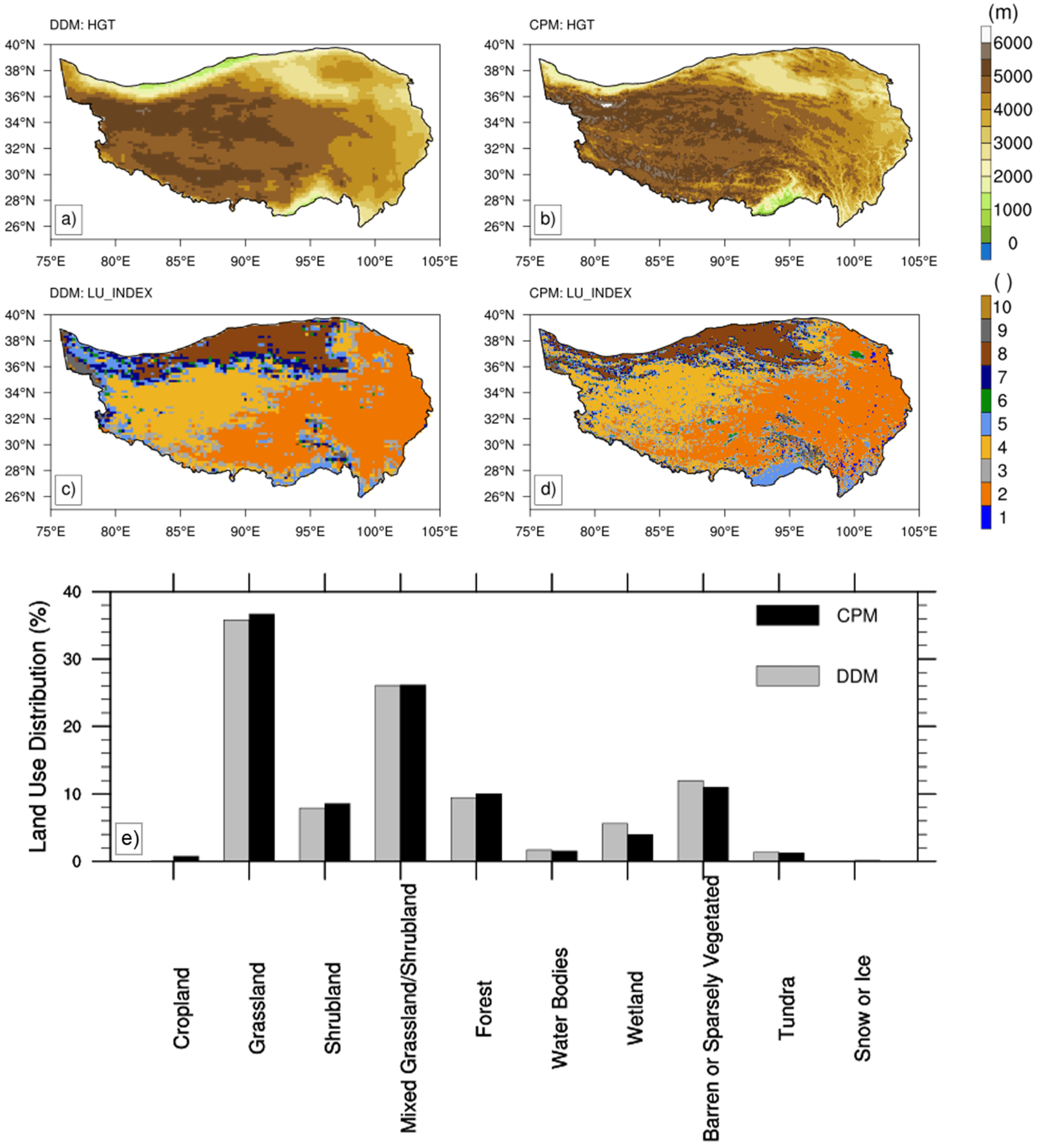
2.1. Model and Configurations

The Weather Research and Forecasting (WRF) model is a next-generation mesoscale numerical weather prediction system (http://www.wrf-model.org/index.php, accessed on 20 June 2021) [59], which was initially developed in the late 1990s and is still being improved today by scientists all over the world. WRF includes several dynamic cores, such as a fully mass- and scalar-conserving flux from the mass coordinate version, as well as many different physical parameterizations (e.g., microphysics, cumulus parameterization, planetary boundary layer, shortwave and longwave radiation, and land-surface models) [51,60,61].
The DDM run (outer domain) covered the entire Eurasian continent with a 28 km horizontal grid spacing, while the CPM run (inner domain) covered the entire TP with a 4 km horizontal grid spacing. The topography of the TP is shown in Figure 1a,b. Clearly, the 4 km resolution topography shows far more detail in terms of mountain tops and valleys, especially in the southern TP.
Following our group’s previous study on DDM and CPM [51], the NCAR (National Center for Atmospheric Research) CAM (Community Atmosphere Model) radiation scheme [62], the WSM6 (WRF Single-Moment 6-class microphysics scheme) [63], Yonsei University planetary boundary layer scheme [64], the Kain–Fritsch convection scheme [65] (used in the DDM run but not in the CPM run), and the Noah LSM (land-surface model) four-layer soil temperature and moisture model [66] were employed in this study too. The specific model configurations are shown in Table 1. We selected 2014 as the research period because the precipitation in this year was close to the climatological mean, which can help avoid the influence of certain extreme conditions and better test the ability of CPM and DDM to simulate ET under the climate mean state. The lateral boundary conditions and sea surface temperature (SST) were provided by the ERA-Interim reanalysis dataset at 6 h intervals. For both DDM and CPM, the simulations were separated into two stages: the first was initialized at 0000 UTC 1 October 2013, ended at 2300 UTC 31 May 2014, and archived in 3 h intervals; and the second was initialized at 0000 UTC 1 June 2014, ended at 2300 UTC 31 December 2014, and archived in 1 h intervals.

2.2. Datasets

Besides the DDM and CPM simulations, a gridded remote sensing dataset (EB), a dataset from off-line simulations (GLDAS), and two large-scale reanalysis datasets (ERA-Interim and ERA5) were adopted for comparison.
The EB dataset (http://data.tpdc.ac.cn, accessed on 20 June 2020) was derived from satellite data and a surface energy balance method for the global land area. It includes daily and monthly datasets from 2000 to 2017, with a 5 km horizontal resolution. This dataset has been proven to be robust across a variety of land-cover types and performs well in providing spatial and temporal information on the water cycle and land–atmosphere interactions for the Chinese landmass [67]. Therefore, EB was used as the reference ET in this study.
GLDAS [68] simulates the ET from four land-surface models driven by a series of conventional and satellite-derived observations. GLDAS products have a spatial resolution of 0.25° × 0.25° and a temporal resolution of 3 h. For a long time, GLDAS has been the only gridded dataset for ET available over the TP [60,69] and has been found to perform well in terms of surface air temperature and precipitation forcing [70].
ERA-Interim and ERA5 are commonly used reanalysis datasets released by the ECMWF (the European Center for Medium-Range Weather Forecasts). ERA-Interim [71] covers the period 1979 to 2019 and has a horizontal resolution of 0.7°. It was produced with a 12 h 4D-Var (four-dimensional variational) data assimilation scheme and an IFS (Integrated Forecast System) release Cy31r2 forecast model. Previous studies have shown that it is the outstanding performer among all reanalysis datasets in describing the water cycle over TP [48,69].
ERA5 [72] is the successor to ERA-Interim, with a temporal resolution of 1 h and horizontal resolution of 0.1°. With a more sophisticated hybrid incremental 4D-Var system [73] and advanced forecast model (IFS release Cy41r2), ERA5 covers a longer period from 1950 to the present day and outputs more meteorological elements. Moreover, its radiative transfer model, land-surface model, and snow data assimilation are all different from those of ERA-Interim. These improvements may have advantages in exploring regions with complex terrain, such as the TP.

2.3. Methods

To intercompare the six datasets with different temporal and spatial resolutions, all of the datasets were first monthly averaged and then interpolated into the same 0.25° grid through the local area averaging method. The comparison was conducted in terms of the annual and seasonal means as well as seasonal variabilities. According to the typical seasonal variation of precipitation over the TP [2], the monthly data were further averaged to the monsoon season (May–September) and the non-monsoon season (October–April).
Since the calculation of ET is directly land-use dependent, we compared the dominant land-use types in the DDM and CPM simulations. There are 24 land-use types for the USGS (United States Geological Survey) categories in the WRF model (http://www2.mmm.ucar.edu/wrf/users/docs/user_guide_V3.8/AWUsersGuideV3.8.pdf, accessed on 20 June 2021) [74]. However, not all of them exist over the TP. To present the categories clearly, we reclassified these land-use types over the TP into 10 categories (cropland, grassland, shrubland, mixed shrubland/grassland, forest, water bodies, wetland, barren or sparsely vegetated, tundra, and snow or ice) (provided in Table 2). The distributions of these 10 categories are shown in Figure 1c–e. Considering that the EB data do not include the underlying surface of water bodies, all comparisons in this study do not consider this surface type. The distributions according to DDM and CPM are quite similar, with very slight differences in percentages for each category (Figure 1c–e). Therefore, the distribution of the 10 dominant categories of CPM can be used in the comparison among the 0.25° grid cells via the nearest neighbor algorithm. To investigate the contributions from each land-use category to the TP average, the ET in the same category was averaged and intercompared among the six datasets.
In addition, to better judge whether the ET deviation from the other five datasets over the dominate land-use categories of TP is significant compared to EB, we also conducted a 99% significance test with the Monte-Carlo method [75], which does not require the data to be normally distributed. The Monte-Carlo method regards the two datasets with sample sizes of n a and n b as a method of randomly extracting n a samples from the total ( n a + n b ) samples, it calculates the absolute value, D i , of the sample mean difference from m resampled group as follows:
D i = | x a i ¯ x b i ¯ |
where x a i ¯ ,   x b i ¯ represent the averaged value of the two new datasets in each group; i = 1 ,   2 ,   3 ,   ,   m ; m is re-sampling times, and m = 10,000 in this study. Then, the obtained D i is sorted from smallest to largest and compared with the original sequence mean difference, D o r i . If the D o r i satisfies the following condition:
D o r i < D α 2   o r   D o r i >   D 1 α 2
where α = 0.01 in this study, it is considered that the samples have passed the 99% Monte-Carlo significance test, and there is a significant difference between the two compared datasets.
Many factors play a key role in the simulation of ET, especially precipitation [76,77,78]. In addition, radiation provides the energy source for ET. However, the benchmark data EB is a satellite-derived dataset and has no other matching variables. Thus, it cannot be used as an attribution reference criterion. In order to explore the factors influencing the deviations of simulated ET, first, EB was used as the standard to find the nearest and farthest datasets to it, and then the nearest one was used as the reference in the comparison and the farthest to explore the source of deviations in attribution analysis (in Section 3.3).
Then, to explore the influence of precipitation on deviations in ET, the deviations of ET (dET) of the selected datasets were separated into those from precipitation (dP) and all other types of deviation (dET-dP), which were obtained from
d A i = A s i A r e f i
where d A i is an abstract symbol, which can be replaced by deviations from ET (mm/d), precipitation (mm/d), net radiation flux (w m−2), or soil temperature (K) in this equation; A s i is the corresponding variable (ET, precipitation, net radiation flux, or soil temperature) of the dataset furthest from the ET value of the EB data (mm/d); A r e f i is the corresponding variable (ET, precipitation, net radiation flux, or soil temperature) of the dataset closest to the ET value of the EB data (mm/d); i is the land-use type range from 1 to 10 without 6 (the water bodies).
To further explore the contributions from radiation and the land-surface model in the non-monsoon season, the dET-dP was further analyzed by comparing deviations from surface net radiation (dR) and soil temperature (dST), which can be calculated using Equation (1). Considering the different units, a relative contribution was defined by normalized deviations, and defined as
d B r j = | d B j | | d B m a x | × 100 %
where d B j is an abstract symbol, which can be replaced by the deviations from net radiation flux (w m−2) or soil temperature (K) in this equation; d B r j is the relative deviation (%) of the corresponding variable (net radiation flux or soil temperature); d B m a x is the maximum deviation of the corresponding variable [net radiation flux (w m−2) or soil temperature (K)] of all nine land-use types (without the water bodies); j is land-use type 9 (the tundra) or 10 (snow or ice).
The relative contributions from surface net radiation (dRr) and the land-surface model (dSTr - dRr) are represented by the magnitudes of the normalized deviations.

3. Results

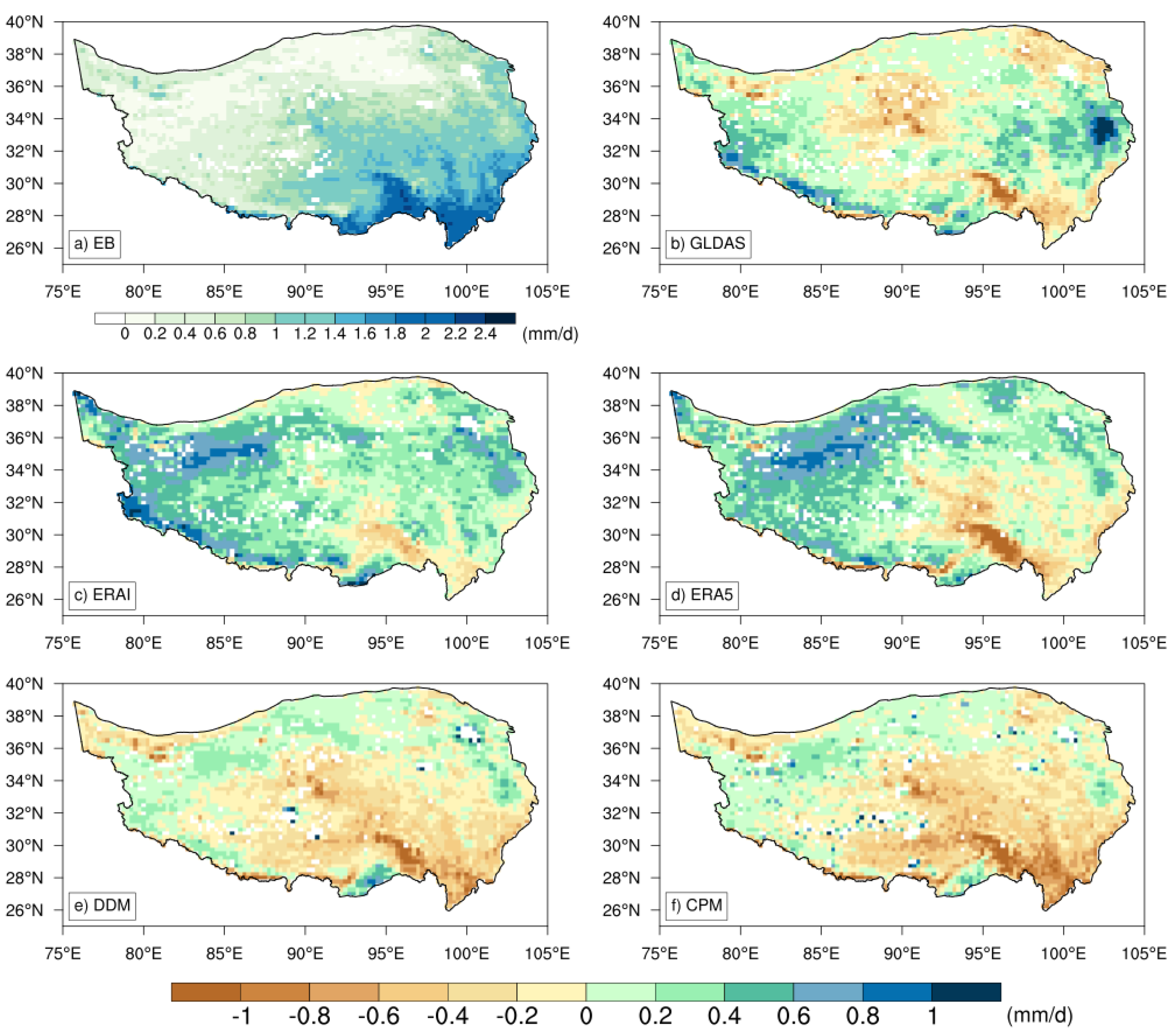
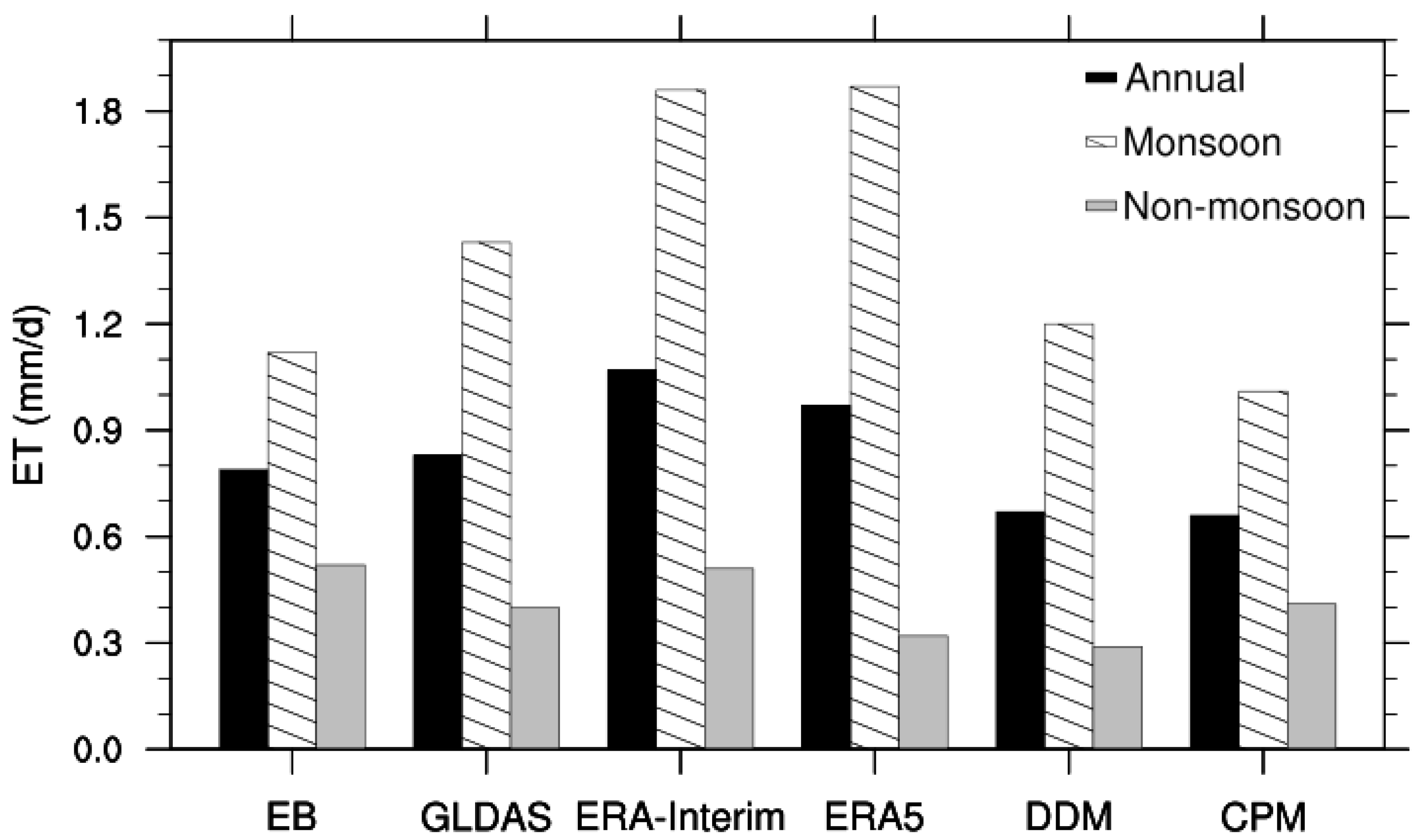
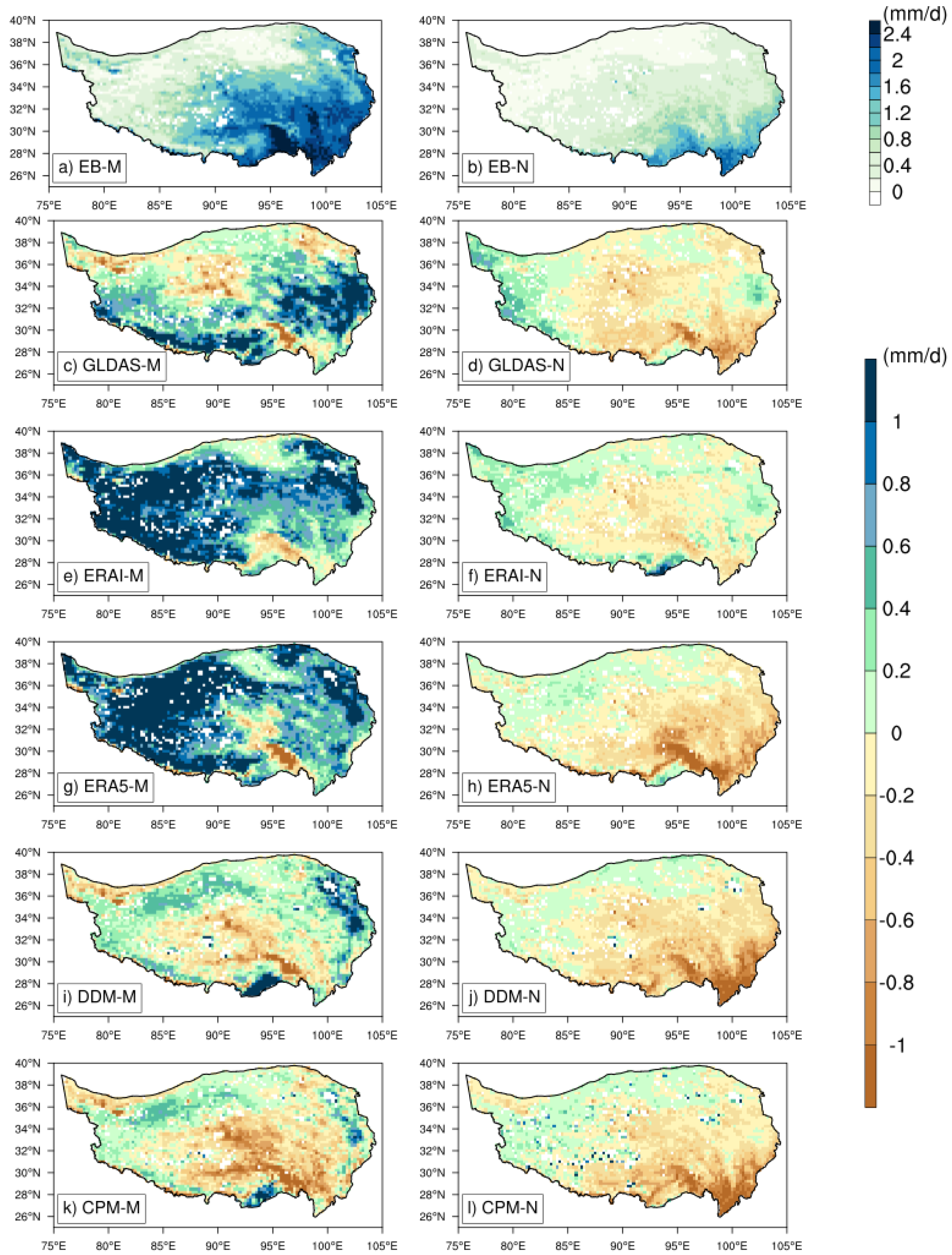
3.1. Annual and Seasonal Mean ET

Figure 2 presents the annual mean distribution of ET in EB and its differences with those of the GLDAS, ERA-Interim, ERA5, DDM, and CPM datasets. EB exhibits a decrease in gradient from the southeastern TP to the northwestern TP. The daily ET reaches 2 mm d−1 in the southeastern TP and is almost down to zero in the northwestern TP (Figure 2a). The spatial distribution is generally in line with the pattern of precipitation over the TP [50,51]. Compared to EB, GLDAS shows a very similar annual mean spatial distribution (Figure 2b). ERA-Interim and ERA5 both significantly overestimate the ET almost for the entire TP (Figure 2c,d). As for the DDM and CPM, the simulations are very similar, both of them producing lower ET than EB in the central and southern regions of the plateau, with CPM being relatively lower than DDM (Figure 2e,f).
Figure 3 shows the annual and seasonal mean ET for the six datasets in 2014 averaged over the TP. Averaged over the TP, EB estimates around 0.79 mm of moisture was evaporated per day in 2014. Broken down, this figure is 1.12 mm d−1 for the monsoon season, which accounts for most of the annual ET, and 0.52 mm d−1 for the non-monsoon season. GLDAS shows obvious deviation in both monsoon season and non-monsoon season in comparison with EB. ERA-Interim and ERA5 have the largest annual deviation, which was mainly from the monsoon season. The DDM and CPM are the closest datasets to EB in the monsoon season (Figure 3 and Table 3), while CPM is the only one that underestimates the ET.
The seasonal mean ET of EB shows a great decrease in the non-monsoon season when compared to that in the monsoon season (Figure 3), which is mainly due to the large decrease in ET over the southern and central TP in the non-monsoon season in comparison with the monsoon season (Figure 4a,b). As for the GLDAS, it is relatively larger in the southeastern TP in the monsoon season and underestimated over the central and southern TP in the non-monsoon season (Figure 4c,d), which results in a balance in the annual mean. The overestimation of ERA-Interim and ERA5 exists almost across the whole TP but is largest in the northwestern TP in the monsoon season (Figure 4e,g). This is unsurprising given the known positive precipitation bias of ERA-Interim and ERA5 over the TP [79]. As for the non-monsoon season, ERA-Interim performs best compared to EB (Figure 4f and Table 3), while ERA5 shows an obvious underestimation especially for the southeastern TP (Figure 4h). DDM and CPM are the closest datasets to EB in the monsoon season (Figure 4i,k); however, in the non-monsoon season, DDM is significantly lower than EB for most of the TP but especially in the southeast (Figure 4j), while CPM ranks as the next best in comparison (Figure 4l and Table 3).

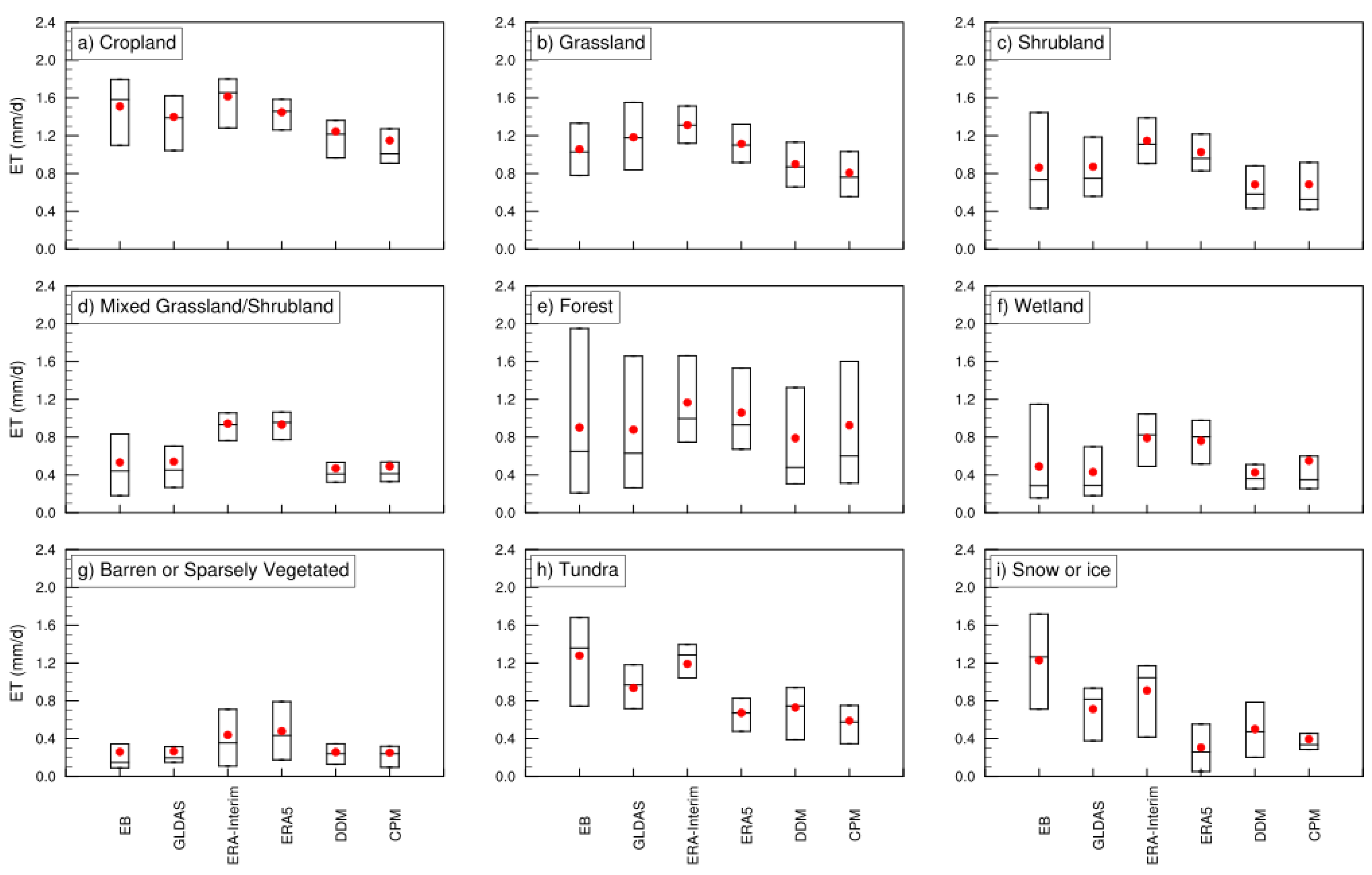
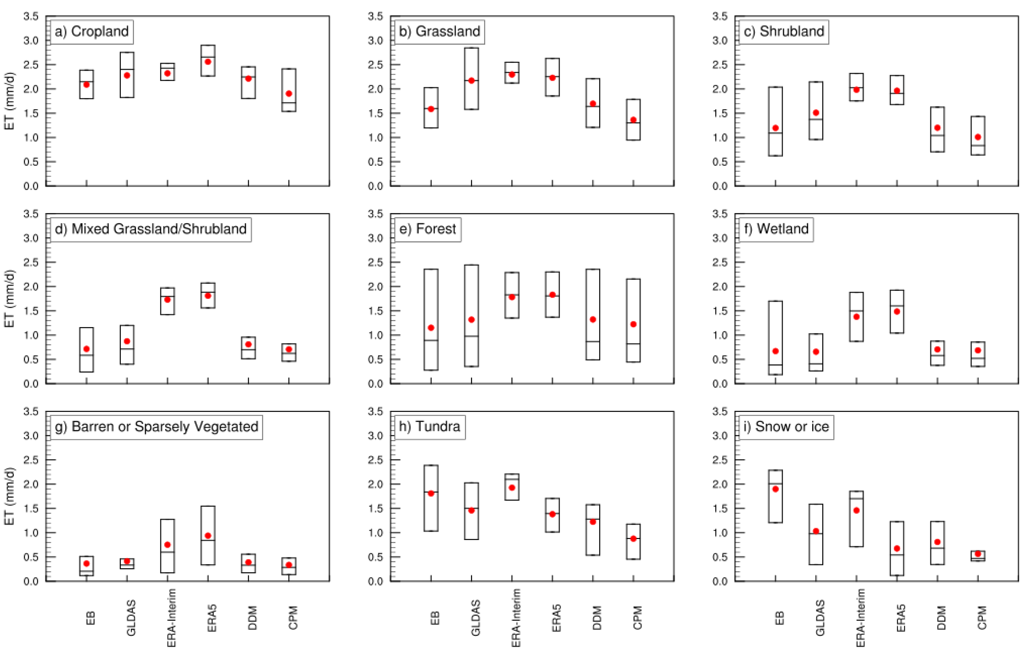
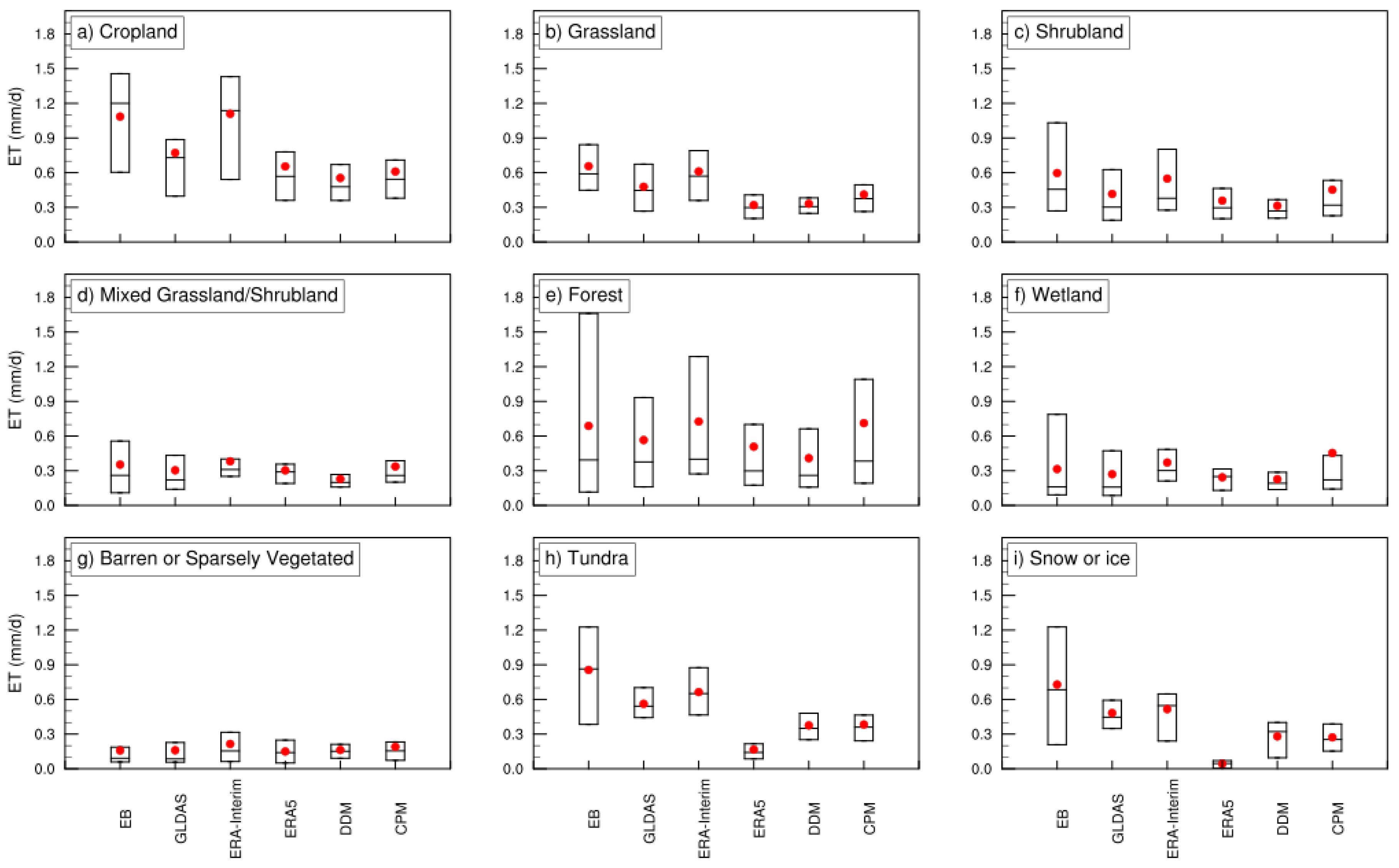
3.2. ET over Dominant Land-Use Categories

Figure 5 presents box-and-whisker plots of the ET of nine land-use types based on the six datasets. The ET values averaged over the monsoon and non-monsoon seasons are given in Figure 6 and Figure 7, respectively. In addition, we also used the Monte-Carlo test to detect whether the simulated ET is significantly different from EB, and the results are shown in Table 4.
Results from Figure 5 indicate that the ET of EB is generally larger over the vegetated ground of the TP. Cropland evaporates the most, with an annual mean value of 1.6 mm d−1, while barren or sparsely vegetated ground only has 0.3 mm d−1. The tundra and snow or ice surfaces present relatively high values for the annual mean. GLDAS shows relatively high consistency with EB in its annual mean over most land-use types, except grassland and tundra. Moreover, although the ET of GLDAS is also seen to be lower than that of EB over the snow/ice land surface, it is not significant (Table 4). The annual mean ET of ERA-Interim and ERA5 are relatively higher than those of EB, especially for the shrubland, mixed grassland/shrubland, forest, and wetland, while DDM and CPM produce lower annual mean ET over vegetated land.
Figure 6 presents the ET value of nine land-use types in the monsoon season. The ET of the EB dataset in the monsoon season is in line with its annual mean situation, the vegetated land evaporates generally more than the barren land. However, the performance of GLDAS in terms of the seasonal mean is unsatisfactory. In the monsoon season, clear overestimation exists for shrubland and grassland, which cover the largest area of the TP (Figure 1). The values provided by ERA-Interim and ERA5 are generally higher than those of other datasets, and this phenomenon exists and is significant for nearly all surfaces in the monsoon season (Table 4). The most obviously overestimated land-surface type of the reanalysis during the monsoon season is mixed grassland/shrubland, with the deviations almost reaching 1.1 mm d−1. Moreover, for DDM and CPM, they both perform much better than other datasets and are closer to the EB data over most surfaces in the monsoon season.
As for the non-monsoon season shown in Figure 7, the tundra and snow or ice surfaces of EB still present relatively high values. Apart from the monsoon season, GLDAS shows large underestimations over cropland in the non-monsoon season (Figure 7 and Table 4) and needs further study as well. ERA-Interim agrees well with EB for nearly all dominant land surfaces in comparison to the non-monsoon season, while the ET in ERA5 is generally lower than that of ERA-Interim, except for wetland and barren or sparsely vegetated land. The lower annual mean ET over vegetated land produced by DDM and CPM (shown in Figure 5) is mainly due to underestimation in the non-monsoon season, especially for DDM. As shown, DDM simulates considerably lower ET over cropland, grassland, shrubland, mixed shrubland/grassland, and forest, while CPM underestimates the ET over cropland, grassland as well as shrubland, which ultimately leads to the underestimation over the whole of the TP. Moreover, the underestimations for tundra and snow/ice in our simulations are significant, as Table 4 shows, and still need to be improved in future simulations.

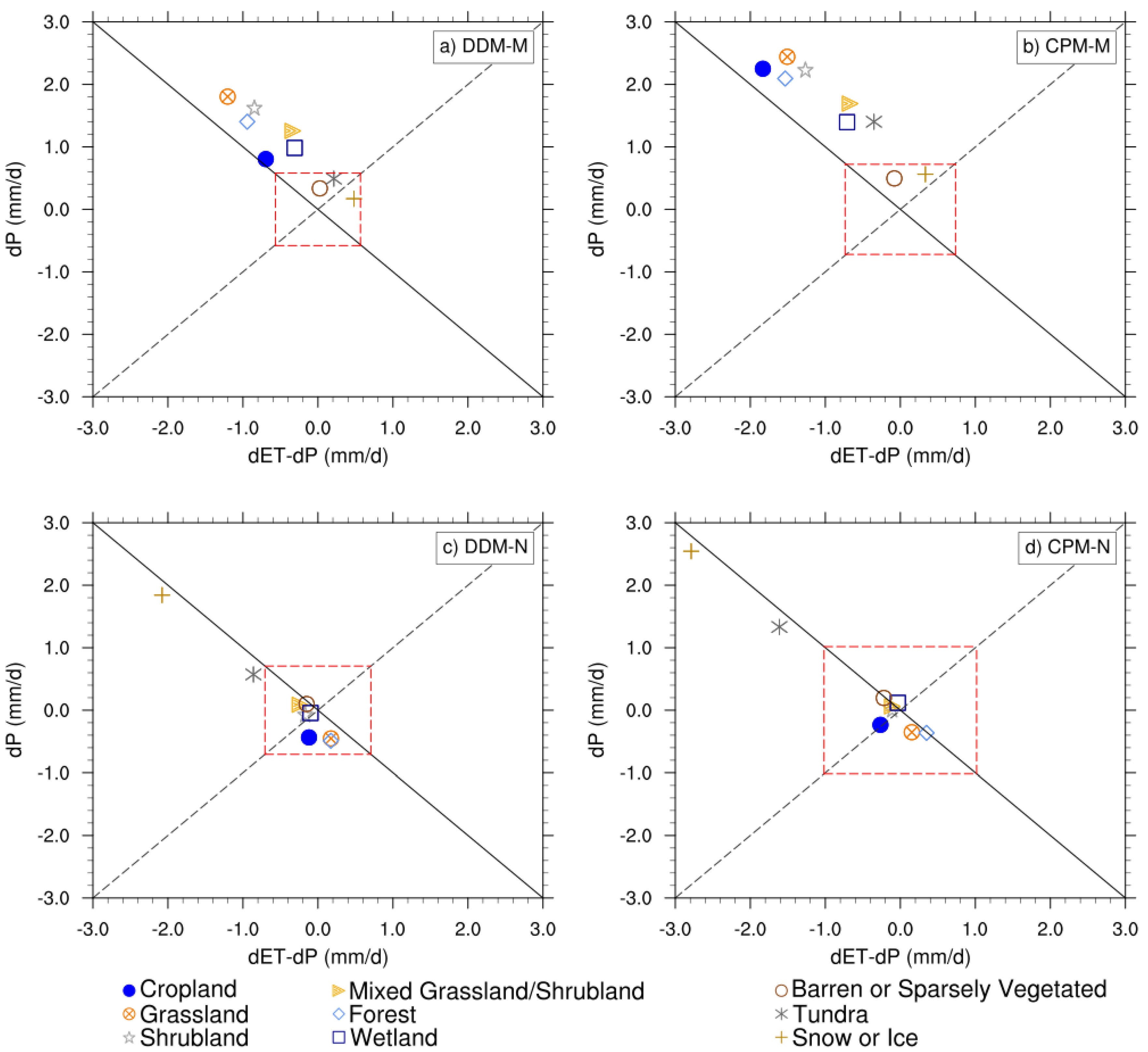
3.3. Attribution of ET Deviations

The DDM- and CPM-simulated ET deviations compared to ERA-Interim and their counterparts from precipitation and other factors are presented in Figure 8. The solid lines represent a constant dET. Most points are located along the solid lines, which demonstrates that the ET deviation is equivalent for most land-cover categories, either in the monsoon or non-monsoon season. The dashed lines combined with the solid lines are used to separate the ET deviation. Points above or below the angle between the dashed and solid lines indicate that the ET deviation is more a result of the precipitation deviation. Points to the left or right indicate that the ET deviation is more a result of the other effects. Meanwhile, the points outside the red dashed box indicate that the deviations from precipitation and other effects are larger than one SD, which means the deviations are significant and cannot be ignored.
In the monsoon season, DDM and CPM agree well with EB. However, ERA-Interim and ERA5 show a large difference. Considering that the boundary conditions and SST in our simulations came from ERA-Interim, exploring its deviation from the two analog values can also lead to a better understanding of where the WRF mode has improved. Thus, DDM and CPM were selected as the reference data to explore the contributing factors to the ET deviations of ERA-Interim in the monsoon season. As shown in Figure 8a,b, all land-use categories in ERA-Interim, except snow or ice, show clear positive deviations in precipitation in comparison with DDM, which indicates that the overestimation of ET in ERA-Interim mainly comes from its large precipitation bias, especially for grassland. Importantly, the two WRF simulations greatly improve the result.
In the non-monsoon season, however, according to the previous analysis, the performances of DDM and CPM are not as good as those of the monsoon season. ERA-Interim shows the best performance and was, therefore, selected as the reference dataset in the non-monsoon season. The deviation from other factors dominates over most land surfaces of the TP, except cropland, grassland, and forest. As shown in Figure 8c,d, although most points are inside the red dashed box, the points for tundra and snow/ice show significant deviation. The other-factor deviations of the snow or ice surface type almost reach −3.0 mm d−1 in CPM. This is in line with the former analysis that precipitation in the monsoon season dominates the ET differences, while other effects such as surface radiation or deviations in the land-surface model play a relatively important role in the non-monsoon season.
As known, in the non-monsoon season, radiation is the dominant forcing that controls the energy balance of melting. To further explore the ET deviations over the tundra and snow/ice surfaces in the non-monsoon season, the relative contributions from surface net radiation deviation and land-surface process deviations were calculated and intercompared (Figure 9). All points are located above the 1:1 line, regardless of DDM or CPM, indicating that the lower ET of these two surfaces is mainly because of the underestimation of radiation, which may cause stronger freezing in the model. Specifically, radiation deviation of the tundra and snow/ice surfaces accounts for 90% and 62%, respectively, while the deviation from the land-surface processes is only 10% and 28%, in DDM. In CPM, the radiation deviation accounts for an even larger proportion, exceeding 90%.

4. Discussion

The ET from remote sensing, off-line and on-line simulations was intercompared over the TP, and some significant deviations were found. There are, however, some drawbacks in this study.

4.1. Uncertainties of Usage Data

Site observations are generally considered to be the direct and most accurate measurement of ET, some atmospheric field experiments have gradually been carried out over the TP since 1970 [80,81,82], and several observation stations have been established [83]. However, due to the limited measurement space of one instrument, which can only measure a limited area within a few hundred to several kilometers [84], the existing observation sites on the TP are too few and insufficient to represent the ET over the whole TP.
Therefore, we selected the high-resolution remote sensing dataset EB, which performs well in land–atmosphere interactions over China, as the benchmark in this study. EB is based on the SEBS method, which requires parameterization of excessive resistance and is sensitive to the errors of air temperature (Ta) and land-surface temperature (Ts) [29]. Unlike the clear-sky conditions, the Ts used for ET calculation in EB can only be obtained by interpolation on cloudy days, and there is always error in interpolation, leading to uncertainty in the EB data. Moreover, many previous studies have noted that the uncertainty of lake parameterization and its impacts on regional climate are non-negligible [50,85,86] in current models; however, the EB data exclude the surfaces covered by lakes, meaning these areas were excluded in the present study, this is also a limitation of the EB dataset. Thus, multiple datasets from remote sensing can be considered for use in the following studies to reduce the uncertainties caused by a single dataset such as EB.
The other five datasets used in the study are all simulated from different models. GLDAS is the “off-line” simulation, which has wide applications in research. The data quality of GLDAS is mainly affected by the driving variables such as temperature, relative moisture, and wind speed [87]. Meanwhile, the lack of feedback mechanism also leads to the lack of the land–atmosphere interaction processes, which increases the uncertainties of GLDAS data as well.
The reanalysis datasets ERA-Interim and ERA5 are objective datasets obtained by conducting quality control on a series of observation data, including site observations, satellites, radar, soundings, aircraft, and ship, and then calculated through the numerical weather forecast data assimilation system. Therefore, these many sources of data bring to the reanalysis not only the advantages of a long-time scale and high spatial resolution but also the problem of poor data continuity [70,79]. The inherent uncertainties also come from the forecast model and data assimilation [88].
As for the “on-line” simulated DDM and CPM datasets, the atmospheric variables such as precipitation are also from simulation rather than being simply input as driving data. The selection of parameters in the model and the uncertainties of the parameterization scheme will influence the accuracy of ET, precipitation, and other variables simulated by DDM and CPM.
In addition, limited by the available computational resources, only a one-year simulation was conducted in this study. Uncovering whether the above results are of climatological significance would require further analysis with multi-year data.

4.2. Parameterizations of the Land-Surface Process

The analysis of the attribution of the ET deviation was only separated into precipitation and radiation deviation at present, with consideration of the water balance and energy balance. As is known, ET consists of soil evaporation, canopy transpiration, and canopy-intercepted water evaporation. Further in-depth study and analysis regarding the impacts of land-surface processes on ET deviations need to be carried out.
Land-surface processes can be solved by parameterization in models; however, previous studies indicated that despite the improvements offered by current simulation capabilities, there are still numerous uncertainties in the parameterization of land-surface processes. The DDM and CPM simulations underestimated the ET over vegetated ground, and the inaccurate representation of canopy light use, interception loss, and root water uptake processes resulting in underestimation of plant transpiration might be the reason for this [89,90]. Furthermore, the difference in the months when the coldest soil temperature appears between the reanalysis data and the WRF simulations (not shown) also indicates an insufficient consideration of snow parameterization, such as the higher snow albedo feedback mechanism, which results in lower incoming radiation and ultimately a cold deviation of the soil temperature [19,51].
Therefore, further investigations are necessary to improve the simulation effect of models and to obtain a more comprehensive and accurate understanding of the ET and water cycle process over the TP.

5. Conclusions

In this study, the ET from satellite merged data (EB), an off-line run (GLDAS), two global climate datasets (ERA5 and ERA-Interim) and two WRF dynamical downscaling simulations (DDM and CPM) were intercompared for a whole year, 2014, which is a normal year for precipitation, over the TP in terms of the annual mean, seasonal variation, and land-use types. Factors contributing to the deviations compared to EB were investigated in order to provide some insight into subsequent model improvements and land–atmosphere interaction simulations. The major conclusions are as follows:
Compared with the EB data, GLDAS generally reproduces the annual mean magnitude and spatial distribution, but seasonal variations are poorly presented. ERA-Interim and ERA5 generally overestimate ET, mainly in the monsoon season. ERA-Interim better reproduces the ET in the non-monsoon season. DDM and CPM perform well in the monsoon season but worse in the non-monsoon season.
ET is underestimated over tundra and snow or ice by all five datasets. GLDAS, ERA5, DDM, and CPM underestimate the ET over cropland, grassland, and shrubland in the non-monsoon season. GLDAS, ERA-Interim, and ERA5 overestimate the ET over grassland and shrubland in the monsoon season. ERA-Interim and ERA5 also overestimate the ET over the other four land-use types in the monsoon season.
Atmospheric forcing plays a dominant role in the simulation of ET. The considerable overestimation of precipitation dominates the ET deviation for the whole year, which is responsible for the particularly high results of ERA-Interim and ERA5 in the monsoon season. In the non-monsoon season, surface net radiation plays a secondary role after precipitation in the simulation of ET. The land-surface model exerts less impact than surface net radiation.

Author Contributions

Conceptualization, methodology: J.D. and Y.G.; validation: J.D., Y.G. and M.Z.; formal analysis, investigation: J.D.; data curation: Y.G.; writing—original draft preparation: J.D.; writing—review and editing: J.D., Y.G. and M.Z. All authors have read and agreed to the published version of the manuscript.

Funding

This research was jointly supported by the Second Tibetan Plateau Scientific Expedition and Research Program (grant 2019QZKK010314) and the Strategic Priority Research Program of the Chinese Academy of Sciences (grant XDA2006010202).

Institutional Review Board Statement

Not applicable.

Informed Consent Statement

Not applicable.

Data Availability Statement

Not applicable.

Acknowledgments

The authors thank Xuelong Chen for his valuable suggestions on this research. The authors thank the National Supercomputer Center in Tianjin for computational resources. The authors appreciate the National Tibetan Plateau Data Center for free access to the EB dataset (http://data.tpdc.ac.cn, 20 June 2021), the National Aeronautics and Space Administration (NASA) for free access to the GLDAS dataset, and the European Center for Medium-Range Weather Forecasts (ECMWF) for free access to the ERA5 and ERA-Interim datasets.

Conflicts of Interest

The authors declare no conflict of interest.

References

  1. Bothe, O.; Fraedrich, K.; Zhu, X.H. Large-scale circulations and Tibetan Plateau summer drought and wetness in a high-resolution climate model. Int. J. Climatol. 2011, 31, 832–846. [Google Scholar] [CrossRef]
  2. Yao, T.D.; Masson-Delmotte, V.; Gao, J.; Yu, W.S.; Yang, X.X.; Risi, C.; Sturm, C.; Werner, M.; Zhao, H.B.; He, Y.; et al. A review of climatic controls on δ18O in precipitation over the Tibetan Plateau: Observations and simulations. Rev. Geophys. 2013, 51, 525–548. [Google Scholar] [CrossRef]
  3. Lu, C.X.; Yu, G.; Xie, G.D. Tibetan Plateau serves as a water tower. IEEE Trans. Geosci. Remote Sens. 2005, 5, 3120–3123. [Google Scholar]
  4. Xu, X.D.; Lu, C.G.; Shi, X.H.; Gao, S.T. World water tower: An atmospheric perspective. Geophys. Res. Lett. 2008, 35, 1–5. [Google Scholar] [CrossRef]
  5. Guo, D.L.; Wang, H.J. The significant climate warming in the northern Tibetan Plateau and its possible causes. Int. J. Climatol. 2011, 32, 1775–1781. [Google Scholar] [CrossRef]
  6. Krause, P.; Biskop, S.; Helmschrot, J.; Flügel, W.-A.; Kang, S.; Gao, T. Hydrological system analysis and modelling of the Nam Co basin in Tibet. Adv. Geosci. 2010, 27, 29–36. [Google Scholar] [CrossRef] [Green Version]
  7. Huntington, T.G. Evidence for intensification of the global water cycle: Review and synthesis. J. Hydrol. 2006, 319, 83–95. [Google Scholar] [CrossRef]
  8. Yin, Y.H.; Wu, S.H.; Zhao, D.S. Past and future spatiotemporal changes in evapotranspiration and effective moisture on the Tibetan Plateau. J. Geophys. Res. Atmos. 2013, 118, 10850–10860. [Google Scholar] [CrossRef]
  9. Kuang, X.X.; Jiao, J.J. Review on climate change on the Tibetan Plateau during the last half century. J. Geophys. Res. 2016, 121, 3979–4007. [Google Scholar] [CrossRef]
  10. Oki, T.; Kanae, S. Global hydrological cycles and world water resources. Science 2006, 313, 1068–1072. [Google Scholar] [CrossRef] [Green Version]
  11. Jung, M.; Reichstein, M.; Ciais, P.; Seneviratne, S.I.; Sheffield, J.; Goulden, M.L.; Bonan, G.; Cescatti, A.; Chen, J.Q.; de Jeu, R.; et al. Recent decline in the global land evapotranspiration trend due to limited moisture supply. Nature 2010, 467, 951–954. [Google Scholar] [CrossRef]
  12. Wang, K.C.; Dickinson, R.E.; Wild, M.; Liang, S.L. Evidence for decadal variation in global terrestrial evapotranspiration between 1982 and 2002:1. Model development. J. Geophys. Res. 2010, 115, D20112. [Google Scholar] [CrossRef] [Green Version]
  13. Douville, H.; Ribes, A.; Decharme, B.; Alkama, R.; Sheffield, J. Anthropogenic influence on multidecadal changes in reconstructed global evapotranspiration. Nat. Clim. Change 2013, 3, 59–62. [Google Scholar] [CrossRef]
  14. Gao, G.; Chen, D.L.; Xu, C.Y.; Simelton, E. Trend of estimated actual evapotranspiration over China during 1960–2002. J. Geophys. Res. 2007, 112, D11120. [Google Scholar] [CrossRef] [Green Version]
  15. Yang, K.; Ye, B.S.; Zhou, D.G.; Wu, B.Y.; Foken, T.; Qin, J.; Zhou, Z.Y. Response of hydrological cycle to recent climate changes in the Tibetan Plateau. Clim. Chang. 2011, 109, 517–534. [Google Scholar] [CrossRef]
  16. Zhang, Y.Q.; Liu, C.M.; Tang, Y.H.; Yang, Y.H. Trends in pan evaporation and reference and actual evapotranspiration across the Tibetan Plateau. J. Geophys. Res. 2007, 112, D12110. [Google Scholar] [CrossRef]
  17. Li, X.P.; Wang, L.; Chen, D.L.; Yang, K.; Wang, A.H. Seasonal evapotranspiration changes (1983–2006) of four large basins on the Tibetan Plateau. J. Geophys. Res. Atmos. 2014, 119, 13079–13095. [Google Scholar] [CrossRef]
  18. Yin, Y.H.; Wu, S.H.; Zhao, D.S.; Zheng, D.; Pan, T. Modeled effects of climate change on actual evapotranspiration in different eco-geographical regions in the Tibetan Plateau. J. Geogr. Sci. 2013, 23, 195–207. [Google Scholar] [CrossRef]
  19. Gao, Y.H.; Xiao, L.H.; Chen, D.L.; Chen, F.; Xu, J.W.; Xu, Y. Quantification of the relative role of land-surface processes and large-scale forcing in dynamic downscaling over the Tibetan Plateau. Clim. Dyn. 2017, 48, 1705–1721. [Google Scholar] [CrossRef]
  20. Wang, X.D.; Zhong, X.H.; Fan, J.R. Spatial distribution of soil erosion sensitivity in the Tibet Plateau. Pedosphere 2005, 15, 465–472. [Google Scholar]
  21. Cui, M.Y.; Wang, J.B.; Wang, S.Q.; Yan, H.; Li, Y.N. Temporal and spatial distribution of evapotranspiration and its influencing factors on Qinghai Tibet Plateau from 1982 to 2014. J. Res. Ecol. 2019, 10, 213–224. [Google Scholar]
  22. Li, Z.Y.; Liu, X.H.; Ma, T.X.; Kejia, D.; Zhou, Q.P.; Yao, B.Q.; Niu, T.L. Retrieval of the surface evapotranspiration patterns in the alpine grassland-wetland ecosystem applying SEBAL model in the source region of the Yellow River, China. Ecol. Modell. 2013, 270, 64–75. [Google Scholar] [CrossRef]
  23. Xue, Z.S.; Lyu, X.G.; Chen, Z.K.; Zhang, Z.S.; Jiang, M.; Zhang, K.; Lyu, Y.L. Spatial and temporal changes of Wetlands on the Qinghai-Tibetan Plateau from the 1970s to 2010s. Chin. Geogr. Sci. 2018, 28, 935–945. [Google Scholar] [CrossRef] [Green Version]
  24. Zhang, Y.S.; Ohata, T.; Kadata, T. Land-surface hydrological processes in the permafrost region of the eastern Tibetan Plateau. J. Hydrol. 2003, 283, 41–56. [Google Scholar] [CrossRef]
  25. Wang, B.B.; Ma, Y.M.; Su, Z.B.; Wang, Y.; Ma, W.Q. Quantifying the evaporation amounts of 75 high-elevation large dimictic lakes on the Tibetan Plateau. Sci. Adv. 2020, 6, eaay8558. [Google Scholar] [CrossRef] [PubMed]
  26. Leuning, R.; Zhang, Y.Q.; Rajaud, A.; Cleugh, H.; Tu, K. A simple surface conductance model to estimate regional evaporation using MODIS leaf area index and the Penman-Monteith equation. Water Resour. Res. 2008, 44, 10. [Google Scholar] [CrossRef]
  27. Su, Z. The surface energy balance system (SEBS) for estimation of turbulent heat fluxes. Hydrol. Earth Syst. Sc. 2002, 6, 85–99. [Google Scholar] [CrossRef]
  28. Chen, X.; Su, Z.; Ma, Y.; Liu, S.; Yu, Q.; Xu, Z. Development of a 10-year (2001–2010) 0.1 data set of land-surface energy balance for mainland China. Atmos. Chem. Phys. 2014, 14, 13097–13117. [Google Scholar] [CrossRef] [Green Version]
  29. Wang, K.C.; Dickinson, R.E. A review of global terrestrial evapotranspiration: Observation, modeling, climatology, and climatic variability. Rev. Geophys. 2012, 50, RG2005. [Google Scholar] [CrossRef]
  30. Yan, H.; Wang, S.Q.; Billesbach, D.; Oechel, W.; Zhang, J.H.; Meyers, T.; Martin, T.A.; Matamala, R.; Baldocchi, D.; Bohrer, G. Global estimation of evapotranspiration using a leaf area index-based surface energy and water balance model. Remote. Sens. Environ. 2012, 124, 581–595. [Google Scholar] [CrossRef] [Green Version]
  31. Li, X.L.; Liang, S.L.; Yuan, W.P.; Yu, G.R.; Chegn, X.; Chen, Y.; Zhao, T.B.; Feng, J.M.; Ma, Z.G.; Ma, M.G. Estimation of evapotranspiration over the terrestrial ecosystems in China. Echohyrology 2014, 7, 139–149. [Google Scholar] [CrossRef]
  32. Chen, J.L.; Wen, J.; Kang, S.C.; Meng, X.H.; Yang, X.Y. The evapotranspiration and environmental controls of typical underlying surfaces on the Qinghai-Tibetan Plateau. Sci. Cold Arid Reg. 2021, 13, 53–61. [Google Scholar]
  33. Xue, B.L.; Wang, L.; Li, X.P.; Yang, K.; Chen, D.L.; Sun, L.T. Evaluation of evapotranspiration estimates for two river basins on the Tibetan Plateau by a water balance method. J. Hydrol. 2013, 492, 290–297. [Google Scholar] [CrossRef]
  34. Giorgi, F.; Francisco, R. Evaluating uncertainties in the prediction of regional climate change. Geophys. Res. Lett. 2000, 27, 1295–1298. [Google Scholar] [CrossRef]
  35. Mearns, L.; Team, N. The North American Regional Climate Change Assessment Program (NARCCAP): Overview of phase II results. In Proceedings of the IOP Conference Series: Earth and Environmental Science, Copenhagen, Denmark, 10–12 March 2009. [Google Scholar]
  36. Gao, Y.H.; Leung, L.R.; Salathe, E.P.; Dominguez, F.; Nijssen, B.; Lettenmaier, D.P. Moisture flux convergence in regional and global climate models: Implications for droughts in the southwestern United States under climate change. Geophys. Res. Lett. 2012, 39, L09711. [Google Scholar] [CrossRef] [Green Version]
  37. Leung, L.R.; Kuo, Y.H.; Tribbia, J. Research needs and directions of regional climate modeling using WRF and CCSM. Bull. Am. Meteorol. Soc. 2006, 87, 1747–1752. [Google Scholar] [CrossRef] [Green Version]
  38. Jacob, D.; Barring, L.; Christensen, O.B.; Christensen, J.H.; de Castro, M.; Deque, M.; Giorgi, F.; Hagemann, S.; Hirschi, M.; Jones, R.; et al. An inter-comparison of regional climate models for Europe: Model performance in present-day climate. Clim. Chang. 2007, 81, 31–52. [Google Scholar] [CrossRef]
  39. Glisan, J.M.; Gutowski, W.J.; Cassano, J.J.; Higgins, M.E. Effects of spectral nudging in WRF on arctic temperature and precipitation simulations. J. Clim. 2013, 26, 3985–3999. [Google Scholar] [CrossRef]
  40. Huang, Z.Y.; Zhong, L.; Ma, Y.M.; Fu, Y.F. Development and evaluation of spectral nudging strategy for the simulation of summer precipitation over the Tibetan Plateau using WRF (v4.0). Geosci. Model Dev. 2021, 14, 2027–2841. [Google Scholar] [CrossRef]
  41. Deque, M.; Jones, R.G.; Wild, M.; Giorgi, F.; Christensen, J.H.; Hassell, D.C.; Vidale, P.L.; Rockel, B.; Jacob, D.; Kjellstrom, E. Global high resolution versus limited area model climate change projections over Europe: Quantifying confidence level from PRUDENCE results. Clim. Dyn. 2005, 25, 653–670. [Google Scholar] [CrossRef]
  42. Gao, X.J.; Xu, Y.; Zhao, Z.C.; Pal, J.S.; Giorgi, F. On the role of resolution and topography in the simulation of East Asia precipitation. Theor. Appl. Climatol. 2006, 86, 173–185. [Google Scholar] [CrossRef]
  43. Giorgi, F.; Bates, G.T.; Nieman, S.J. Simulation of the arid climate of the southern Great Basin using a regional climate model. Bull. Am. Meteorol. Soc. 1992, 73, 1807–1822. [Google Scholar] [CrossRef] [Green Version]
  44. Laprise, R.; Caya, D.; Giguere, M.; Bergeron, G.; Boer, G.J.; McFarlane, N.A. Climate and climate change in western Canada as simulated by the Canadian regional climate model. Atmos. Ocean 1998, 36, 119–167. [Google Scholar] [CrossRef]
  45. Li, S.S.; Lyu, S.H.; Gao, Y.H.; Zhang, Y. Effect of different horizontal resolution on simulation of precipitation in Qilian Mountain. Plateau Meteor. 2005, 24, 496–502. [Google Scholar]
  46. Mearns, L.O.; Gutowski, W.; Jones, R.; Leung, R.; Yun, Q. A regional climate change assessment program for North America. Eos. Trans. Am. Geophys. Union 2009, 90, 311. [Google Scholar] [CrossRef]
  47. Zhang, Y.X.; Duliere, V.; Mote, P.W.; Salathe, E.P. Evaluation of WRF and HadRM mesoscale climate simulations over the U.S. Pacific Northwest. J. Clim. 2009, 22, 5511–5526. [Google Scholar] [CrossRef] [Green Version]
  48. Gao, Y.H.; Xu, J.W.; Chen, D.L. Evaluation of WRF mesoscale climate simulations over the Tibetan Plateau during 1979–2011. J. Clim. 2015, 28, 2823–2841. [Google Scholar] [CrossRef] [Green Version]
  49. Lin, C.G.; Chen, D.L.; Yang, K.; Ou, T.H. Impact of model resolution on simulating the water vapor transport through the central Himalayas: Implication for models’ wet bias over the Tibetan Plateau. Clim. Dyn. 2018, 51, 3195–3207. [Google Scholar] [CrossRef] [Green Version]
  50. Gao, Y.H.; Chen, F.; Miguez-Macho, G.; Li, X. Understanding precipitation recycling over the Tibetan Plateau using tracer analysis with WRF. Clim. Dyn. 2020, 55, 2921–2937. [Google Scholar] [CrossRef]
  51. Gao, Y.H.; Chen, F.; Jiang, Y.S. Evaluation of a convection-permitting modeling of precipitation over the Tibetan Plateau and its influences on the simulation of snow-cover fraction. J. Hydrometeorol. 2020, 21, 1531–1548. [Google Scholar] [CrossRef]
  52. Arakawa, A. The cumulus parameterization problem: Past, present, and future. J. Clim. 2004, 17, 2493–2525. [Google Scholar] [CrossRef] [Green Version]
  53. Brockhaus, P.; Lüthi, D.; Schär, C. Aspects of the diurnal cycle in a regional climate model. Meteorol. Z. 2008, 17, 433–443. [Google Scholar] [CrossRef]
  54. Prein, A.F.; Langhans, W.; Fosser, G.; Ferrone, A.; Ban, N.; Goergen, K.; Keller, M.; Tolle, M.; Gutjahr, O.; Feser, F. A review on regional convection-permitting climate modeling: Demonstrations, prospects, and challenges. Rev. Geophys. 2015, 53, 323–361. [Google Scholar] [CrossRef] [PubMed] [Green Version]
  55. Romps, D.M. A direct measure of entrainment. J. Atmos. Sci. 2010, 67, 1908–1927. [Google Scholar] [CrossRef]
  56. Song, X.; Zhang, G.J. Convection parameterization, tropical pacifific double ITCZ, and upper-ocean biases in the NCAR CCSM3: Part I. Climatology and atmospheric feedback. J. Clim. 2009, 22, 4299–4315. [Google Scholar] [CrossRef]
  57. Ou, T.H.; Chen, D.L.; Chen, X.C.; Lin, C.G.; Yang, K.; Lai, H.W.; Zhang, F.Q. Simulation of summer precipitation diurnal cycles over the Tibetan Plateau at the gray-zone grid spacing for cumulus parameterization. Clim. Dyn. 2020, 54, 3525–3539. [Google Scholar] [CrossRef] [Green Version]
  58. Prein, A.F.; Gobiet, A.; Suklitsch, M.; Truhetz, H.; Awan, N.K.; Keuler, K.; Georgievski, G. Added value of convection permitting seasonal simulations. Clim. Dyn. 2013, 41, 2655–2677. [Google Scholar] [CrossRef] [Green Version]
  59. Skamarock, W.C. Evaluating mesoscale NWP models using kinetic energy spectra. Mon. Weather Rev. Mon. 2004, 132, 3019–3032. [Google Scholar] [CrossRef]
  60. Gao, Y.H.; Leung, L.R.; Zhang, Y.X.; Cuo, L. Changes in moisture flux over the Tibetan Plateau during 1979–2011: Insights from a high-resolution simulation. J. Clim. 2015, 28, 4185–4197. [Google Scholar] [CrossRef]
  61. Huang, M.; Huang, B.; Gu, L.J.; Huang, H.L.A.; Goldberg, M.D. Parallel GPU architecture framework for the WRF single moment 6-class microphysics scheme. Comput. Geosci. 2015, 83, 17–26. [Google Scholar] [CrossRef]
  62. Collins, W.D.; Rasch, P.J.; Boville, B.A.; Hack, J.J.; McCaa, J.R. Description of the NCAR community atmosphere model (CAM 3.0). NCAR Tech. 2004, 226, 1326–1334. [Google Scholar]
  63. Hong, S.Y.; Lim, J.O.J. The WRF single-moment 6-class microphysics scheme (WSM6). J. Korean Meteorol. Soc. 2006, 42, 129–151. [Google Scholar]
  64. Hong, S.Y.; Pan, H.L. Nonlocal boundary layer vertical diffusion in a medium-range forecast model. Mon. Weather Rev. 1996, 124, 2322–2339. [Google Scholar] [CrossRef] [Green Version]
  65. Kain, J.S. The Kain–Fritsch convective parameterization: An update. J. Appl. Meteor. 2004, 43, 170–181. [Google Scholar] [CrossRef] [Green Version]
  66. Chen, F.; Dudhia, J. Coupling an advanced land surface-hydrology model with the Penn State-NCAR MM5 modeling system. Part I: Model implementation and sensitivity. Mon. Weather Rev. 2011, 129, 569–585. [Google Scholar] [CrossRef] [Green Version]
  67. Surface Energy Balance Based Global Land Evapotranspiration (EB-ET 2000-2017). Available online: http://data.tpdc.ac.cn (accessed on 25 June 2021).
  68. Rodell, M.; Houser, P.R.; Jambor, U.; Gottschalck, J.; Mitchell, K.; Meng, C.J.; Arsenault, K.; Cosgrove, B.; Radakovich, J.; Bosilovich, M.; et al. The global land data assimilation system. Bull. Am. Meteor. Soc. 2004, 85, 381–394. [Google Scholar] [CrossRef] [Green Version]
  69. Gao, Y.H.; Cuo, L.; Zhang, Y.X. Changes in moisture flux over the Tibetan Plateau during 1979–2011 and possible mechanisms. J. Clim. 2014, 27, 1876–1893. [Google Scholar] [CrossRef]
  70. Wang, A.H.; Zeng, X.B. Evaluation of multi-reanalysis products with in situ observations over the Tibetan Plateau. J. Geophys. Res. 2012, 117, D05102. [Google Scholar]
  71. Dee, D.P.; Uppala, S.M.; Simmons, A.J.; Berrisford, P.; Poli, P.; Kobayashi, S.; Andrae, U.; Balmaseda, M.A.; Balsamo, G.; Bauer, P.; et al. The ERA-Interim reanalysis: Configuration and performance of the data assimilation system. Q. J. R. Meteor. Soc. 2011, 137, 553–597. [Google Scholar] [CrossRef]
  72. Hersbach, H.; Bell, B.; Berrisford, P.; Hirahara, S.; Horanyi, A.; Munoz-Sabater, J.; Nicolas, J.; Peubey, C.; Radu, R.; Schepers, D.; et al. The ERA5 global reanalysis. Q. J. R. Meteor. Soc. 2020, 146, 1999–2049. [Google Scholar] [CrossRef]
  73. Bonavita, M.; Hólm, E.; Isaksen, L.; Fisher, M. The evolution of the ECMWF hybrid data assimilation system. Q. J. R. Meteor. Soc. 2016, 142, 287–303. [Google Scholar] [CrossRef]
  74. NCAR. ARW version 3 modeling system user’s guide. Natl. Cent. Atmos. Res. Doc. 2017, 434, 85–87. [Google Scholar]
  75. Shi, N.; Wei, F.Y.; Feng, G.L.; Shen, T.L. Monte Carlo test method and application in correlation analysis and comprehensive analysis of meteorological field (in Chinese). J. Nanjing Ins. Meteorol. 1997, 20, 355–359. [Google Scholar]
  76. Alves, M.D.; de Carvalho, L.G.; Vianello, R.L.; Sediyama, G.C.; de Oliveira, M.S.; de Sa, A. Geostatistical improvements of evapotranspiration spatial information using satellite land surface and weather stations data. Theor. Appl. Climatol. 2013, 113, 155–174. [Google Scholar] [CrossRef]
  77. Brutsaert, W. Energy fluxes at the Earth’s surface. In Evaporation into the Atmosphere. Environmental Fluid Mechanics; Springer: Dordrecht, The Netherlands, 1982; pp. 128–153. [Google Scholar]
  78. Montaldo, N.; Oren, R. Changing seasonal rainfall distribution with climate directs contrasting impacts at evapotranspiration and water yield in the western Mediterranean region. Earth Future 2018, 6, 841–885. [Google Scholar] [CrossRef]
  79. Bao, X.H.; Zhang, F.Q. Evaluation of NCEP-CFSR, NCEP-NCAR, ERA-Interim, and ERA-40 reanalysis datasets against independent sounding observations over the Tibetan Plateau. J. Clim. 2013, 26, 206–214. [Google Scholar] [CrossRef] [Green Version]
  80. Tao, S.; Luo, S.; Zhang, H. The Qinghai-Xizang Plateau meteorological experiment (Qxpmex) May–August 1979. In Proceedings of the International Symposium on the Qinghai-Xizang Plateau and Mountain Meteorology, Beijing, China, 20–24 March 1986. [Google Scholar]
  81. Wang, J. Land surface process experiments and interaction study in China-From HEIFE to IMGRASS and GAME-TIBET/TIPEX. Plateau Meteorol. 1999, 18, 280–294. [Google Scholar]
  82. Ma, Y.; Yao, T.; Wang, J. Experimental study of energy and water cycle in Tibetan plateau—The progress introduction on the study of GAME/Tibet and CAMP/Tibet. Plateau Meteorol. 2006, 25, 344–351. [Google Scholar]
  83. Ma, Y.M.; Hu, Z.Y.; Xie, Z.P.; Ma, W.Q.; Wang, B.B.; Chen, X.L.; Li, M.S.; Zhong, L.; Sun, F.L.; Gu, L.L.; et al. A long-term dataset of hourly integrated land–atmosphere interaction observations on the Tibetan Plateau. Earth Syst. Sci. Data 2020, 12, 2937–2957. [Google Scholar] [CrossRef]
  84. Yao, Y.J.; Liang, S.L.; Li, X.L.; Chen, J.Q.; Wang, K.C.; Jia, K.; Cheng, J.; Jiang, B.; Fisher, J.B.; Mu, Q.Z.; et al. A satellite-based hybrid algorithm to determine the Priestley–Taylor parameter for global terrestrial latent heat flux estimation across multiple biomes. Remote Sens. Environ. 2015, 165, 216–233. [Google Scholar] [CrossRef] [Green Version]
  85. Qiao, B.J.; Zhu, L.P.; Yang, R.M. Temporal-spatial differences in lake water storage changes and their links to climate change throughout the Tibetan Plateau. Remote Sens. Environ. 2019, 222, 232–243. [Google Scholar] [CrossRef]
  86. Wang, B.B.; Ma, Y.M.; Wang, Y.; Su, Z.B.; Ma, W.Q. Significant differences exist in lake-atmosphere interactions and the evaporation rates of high-elevation small and large lakes. J. Hydrol. 2019, 573, 220–234. [Google Scholar] [CrossRef]
  87. Dirmeyer, P.A.; Gao, X.; Zhao, M.; Guo, Z.C.; Oki, T.K.; Hanasaki, N. GSWP-2: Multimodel analysis and implications for our perception of the land surface. Bull. Am. Meteorol. Soc. 2006, 87, 1381–1397. [Google Scholar] [CrossRef] [Green Version]
  88. Hodges, K.I.; Lee, R.W.; Bengtsson, L. A comparison of extratropical cyclones in recent reanalyses ERA-Interim, NASA MERRA, NCEP CFSR, and JRA-25. J. Clim. 2011, 24, 4888–4906. [Google Scholar] [CrossRef]
  89. Lian, X.; Piao, S.L.; Huntingford, C.; Li, Y.; Zeng, Z.Z.; Wang, X.H.; Ciais, P.; McVicar, T.R.; Peng, S.S.; Ottle, C.; et al. Partitioning global land evapotranspiration using CMIP5 models constrained by observations. Nat. Clim. Chang. 2018, 8, 640–646. [Google Scholar] [CrossRef]
  90. Tanaka, N.; Kume, T.; Yoshifuji, N.; Tanaka, K.; Takizawa, H.; Shiraki, K.; Tantasirin, C.; Tangtham, N.; Suzuki, M. A review of evapotranspiration estimates from tropical forests in Thailand and adjacent regions. Agric. For. Meteorol. 2008, 148, 807–819. [Google Scholar] [CrossRef]
Figure 1. (a,b) The distribution of topography (unit: m), and (c,d) the dominant land-use categories over the Tibetan Plateau (TP). Panels (a,c) are from DDM (dynamical downscaling modeling), and panels (b,d) are from CPM (convection-permitting modeling). (e) The land-use distribution (unit: %) of ten dominant categories. In (ce), the numbers 1–10 stand for cropland, grassland, shrubland, mixed grassland/shrubland, forest, water bodies, wetland, barren or sparsely vegetated, tundra, snow or ice, respectively.
Water 13 02096 g001
Figure 2. Distribution of the daily terrestrial evapotranspiration (ET) in 2014 in the (a) EB data (units: mm/d) and (bf) the deviation from the EB distribution in the (b) GLDAS, (c) ERA-Interim, (d) ERA5, (e) DDM and (f) CPM data.
Water 13 02096 g002
Figure 3. The annual and monsoon/non-monsoon seasonal mean ET in 2014 from the EB, GLDAS, ERA-Interim, ERA5, DDM, and CPM data averaged over the TP (units: mm/d).
Water 13 02096 g003
Figure 4. Distributions of the daily ET from the (a,b) EB data (units: mm/d), and (cl) the differences of the (c,d) GLDAS, (e,f) ERA-Interim, (g,h) ERA5, (i,j) DDM, and (k,l) CPM data compared to EB, averaged over the monsoon (left-hand panels) and non-monsoon (right-hand panels) seasons.
Water 13 02096 g004
Figure 5. Box-and-whisker plots of ET of nine land-use categories based on six datasets averaged in 2014: (a) cropland; (b) grassland; (c) shrubland; (d) mixed grassland/shrubland; (e) forest; (f) wetland; (g) barren or sparsely vegetated; (h) tundra; (i) snow or ice (units: mm/d). The top and bottom of each box are the 20th and 80th percentiles in grid cells with the same land-use type. The lines in each box represent the median; red dots represent the mean.
Water 13 02096 g005
Figure 6. Box-and-whisker plots of ET of nine land-use categories based on six datasets for the monsoon season in 2014: (a) cropland; (b) grassland; (c) shrubland; (d) mixed grassland/shrubland; (e) forest; (f) wetland; (g) barren or sparsely vegetated; (h) tundra; (i) snow or ice (units: mm/d). The top and bottom of each box are the 20th and 80th percentiles in grid cells with the same land-use type. The lines in each box represent the median; red dots represent the mean.
Water 13 02096 g006
Figure 7. Box-and-whisker plots of ET of nine land-use categories based on six datasets for the non-monsoon season in 2014: (a) cropland; (b) grassland; (c) shrubland; (d) mixed grassland/shrubland; (e) forest; (f) wetland; (g) barren or sparsely vegetated; (h) tundra; (i) snow or ice (units: mm/d). The top and bottom of each box are the 20th and 80th percentiles in grid cells with the same land-use type. The lines in each box represent the median; red dots represent the mean.
Water 13 02096 g007
Figure 8. Deviations (monsoon: ERA-Interim minus DDM or CPM; non-monsoon: DDM or CPM minus ERA-Interim) in ET (units: mm/d) from precipitation and other factors for each land-use category in the (a,b) monsoon and (c,d) non-monsoon seasons. The ordinate is the ET deviation from precipitation, the abscissa is the ET deviation from the other effects. The black solid line indicates 1:1 correspondence of the first and third quadrants, and the gray dashed line indicates 1:1 correspondence of the second and fourth quadrants. The red dashed box indicates the SD from precipitation and other effects.
Water 13 02096 g008
Figure 9. Relative contributions (normalized deviations between DDM (dynamical downscaling modeling) or CPM (convection-permitting modeling) and ERA-Interim) from surface net radiance deviation and land-surface processes deviation (unit: %) for tundra and snow or ice land-use categories in the non-monsoon season. The ordinate is the deviation from radiance; the abscissa is deviation from the land-surface processes. The black solid line indicates 1:1 correspondence of the first and third quadrants.
Water 13 02096 g009
Table 1. The Weather Research and Forecasting (WRF) model configurations for dynamical downscaling modeling (DDM) and convection-permitting modeling (CPM).
WRF 3.8DDMCPM
Domain RegionEurasian continent (centered at (92.8°E, 37.8°N))Tibetan Plateau (75-105°E, 26-40°N)
Grid Cells280 × 184750 × 414
Horizontal Grid Spacing28 km4 km
Vertical Levels27
Radiation SchemeCAM (Community Atmosphere Model) [62]
Microphysics SchemeWSM6 (WRF Single-Moment 6-class microphysics scheme) [63]
Planetary Boundary Layer SchemeYonsei University [64]
Convection SchemeKain-Fritsch [65]Explicit
Land Surface ModelNoah [66]
Boundary Conditions and SSTERA-Interim reanalysis
Table 2. Reclassified 10-category land-use categories.
Land Use CategoryLand Use DescriptionUSGS (United States Geological Survey) [74]
1Cropland2–6
2Grassland7
3Shrubland8
4Mixed Shrubland/Grassland9-10
5Forest11–15
6Water Bodies16
7Wetland17-18
8Barren or Sparsely Vegetated19
9Tundra20–23
10Snow or Ice24
Table 3. The mean ET from the EB, GLDAS, ERA-Interim, ERA5, DDM, and CPM data, and the standard deviation (SD), the root-mean-square error (RMSE), and spatial correlation coefficients (CORR) of GLDAS, ERA-Interim, ERA5, DDM, and CPM compared to EB.
EBGLDASERA-InterimERA5DDMCPM
Value (unit: mm/d)Ann0.790.831.070.970.670.66
Monsoon1.121.431.861.871.201.01
Non-Monsoon0.520.400.510.320.290.41
SDAnn0.530.530.360.430.410.47
Monsoon0.730.940.610.630.760.63
Non-Monsoon0.410.300.250.380.200.45
RMSEAnn---0.340.410.420.330.38
Monsoon---0.650.890.950.460.47
Non-Monsoon---0.300.210.370.380.38
CORRAnn---0.940.950.910.950.93
Monsoon---0.940.920.910.950.94
Non-Monsoon---0.900.950.870.900.84
Table 4. The Monte-Carlo significance test of ET at confidence level of 99% over nine land-use categories of GLDAS, ERA-Interim, ERA5, DDM, and CPM compared to EB. * Indicates that the value has passed the 99% significance test, which means the ET is significantly different from that of EB over the corresponding land-surface type.
99% Monte-Carlo Test
GLDASERA-InterimERA5DDMCPM
CroplandAnn *
Monsoon *
Non-Monsoon* ***
GrasslandAnn*****
Monsoon*****
Non-Monsoon*****
ShrublandAnn ****
Monsoon*** *
Non-Monsoon* ***
Mixed Shrubland/GrasslandAnn ***
Monsoon****
Non-Monsoon* **
ForestAnn **
Monsoon **
Non-Monsoon* **
WetlandAnn **
Monsoon **
Non-Monsoon
Barren or Sparsely VegetatedAnn **
Monsoon **
Non-Monsoon *
TundraAnn* ***
Monsoon* ***
Non-Monsoon*****
Snow or IceAnn ***
Monsoon* ***
Non-Monsoon *
Publisher’s Note: MDPI stays neutral with regard to jurisdictional claims in published maps and institutional affiliations.

