Article

Improving Accuracy and Robustness of Space-Time Image Velocimetry (STIV) with Deep Learning

1
Hydro Technology Institute Co., Ltd., Osaka 5306126, Japan
2
Construction Engineering Research Institute, Kobe 6570011, Japan
*
Author to whom correspondence should be addressed.
Water 2021, 13(15), 2079; https://doi.org/10.3390/w13152079
Submission received: 29 June 2021 / Revised: 24 July 2021 / Accepted: 29 July 2021 / Published: 30 July 2021
(This article belongs to the Special Issue Research of River Flooding)

Abstract

:
Image-based river flow measurement methods have been attracting attention because of their ease of use and safety. Among the image-based methods, the space-time image velocimetry (STIV) technique is regarded as a powerful tool for measuring the streamwise flow because of its high measurement accuracy and robustness. However, depending on the image shooting environment such as stormy weather or nighttime, the conventional automatic analysis methods may generate incorrect values, which has been a problem in building a real-time measurement system. In this study, we tried to solve this problem by incorporating the deep learning method, which has been successful in the field of image analysis in recent years, into the STIV method. The case studies for the three datasets indicated that deep learning can improve the efficiency of the STIV method and can continuously improve performance by learning additional data. The proposed method is suitable for building a real-time measurement system because it has no tuning parameters that need to be adjusted according to the shooting conditions and the calculation speed is fast enough for real-time measurement.

1. Introduction

The frequent occurrence of flood disasters in recent years has increased the importance of accumulating basic hydrological data such as rainfall, water level, and river discharge, which are fundamental to river disaster countermeasures [1,2]. Non-contact automated observation systems are indispensable from a labor and cost standpoint to constantly collect accurate data on water levels and river flow at multiple points, even during large floods [3]. However, compared to water level observation, an automatic river flood observation system has not yet been established, and in Japan, this is generally measured manually using floats [4,5]. To overcome this situation, the momentum for unmanned and labor-saving flow observation has been growing in recent years in Japan, shown by projects such as the Innovative River Technology Project [6] led by the Ministry of Land, Infrastructure, Transport and Tourism (MLIT). In the project, comparative research has been conducted for practical applications of recently proposed flow measurement methods such as ADCP (Acoustic Doppler Current Profiler) [7,8,9], SVR (Surface Velocity Radars) [10,11], and image analysis methods [12,13,14]. The project is underway at three first class rivers at present. Of the above methods, the image-based method offers significant economic advantages over other methods because it can use existing camera equipment installed for river monitoring. Furthermore, video images taken from a drone can be used to measure a variety of river surface flows at arbitrary locations.
Image analysis methods include the particle tracking velocimetry (PTV) [15], large-scale particle image velocimetry (LSPIV) [16,17], optical flow method [18] and space-time image velocimetry (STIV) [19,20,21,22,23]. Among these, STIV, which is the subject of this research, has recently been put to practical use in flow observation due to its robustness of measurement and efficiency of calculation, and the software (Hydro-STIV) [24] developed mainly by the authors is now available. In STIV, a search line of arbitrary length is set in the mainstream direction of the image, and the flow velocity is calculated from the gradient of the striped pattern that appears in the space-time image (STI) generated by stacking the image intensity information in the time direction. The advantages of STIV over other methods are that it can analyze images even with a small depression angle of about two degrees by paying attention to the time- and line-averaged streamwise velocity component. On the other hand, in STIV, the mainstream direction needs to be known to set the search line along the mainstream direction. However, since the velocity component perpendicular to the cross section is important in discharge measurements, the direction of the search line can be determined from the cross section setting in many cases except for complex curved parts.
So far, various methods have been proposed for automatically detecting the pattern gradient, such as the gradient tensor method [19], QESTA [25], and masked 2D Fourier spectra method [21,26]. These methods have been used in the surveying work of river flow measurements in the actual field, but problems occasionally occur when the observation environment is not appropriate, such as in stormy weather conditions and during the night. In such cases, it becomes necessary to manually adjust the pattern gradient. To build a reliable real-time measurement system [27], it is important to develop a robust pattern gradient detection method that does not require manual parameter adjustment. To this end, we used a deep learning method, which has achieved remarkable results in recent years in image analysis such as pattern recognition, to improve the robustness of pattern gradient detection and to fully automate the process without manual parameter adjustment.

2. Outline of STIV

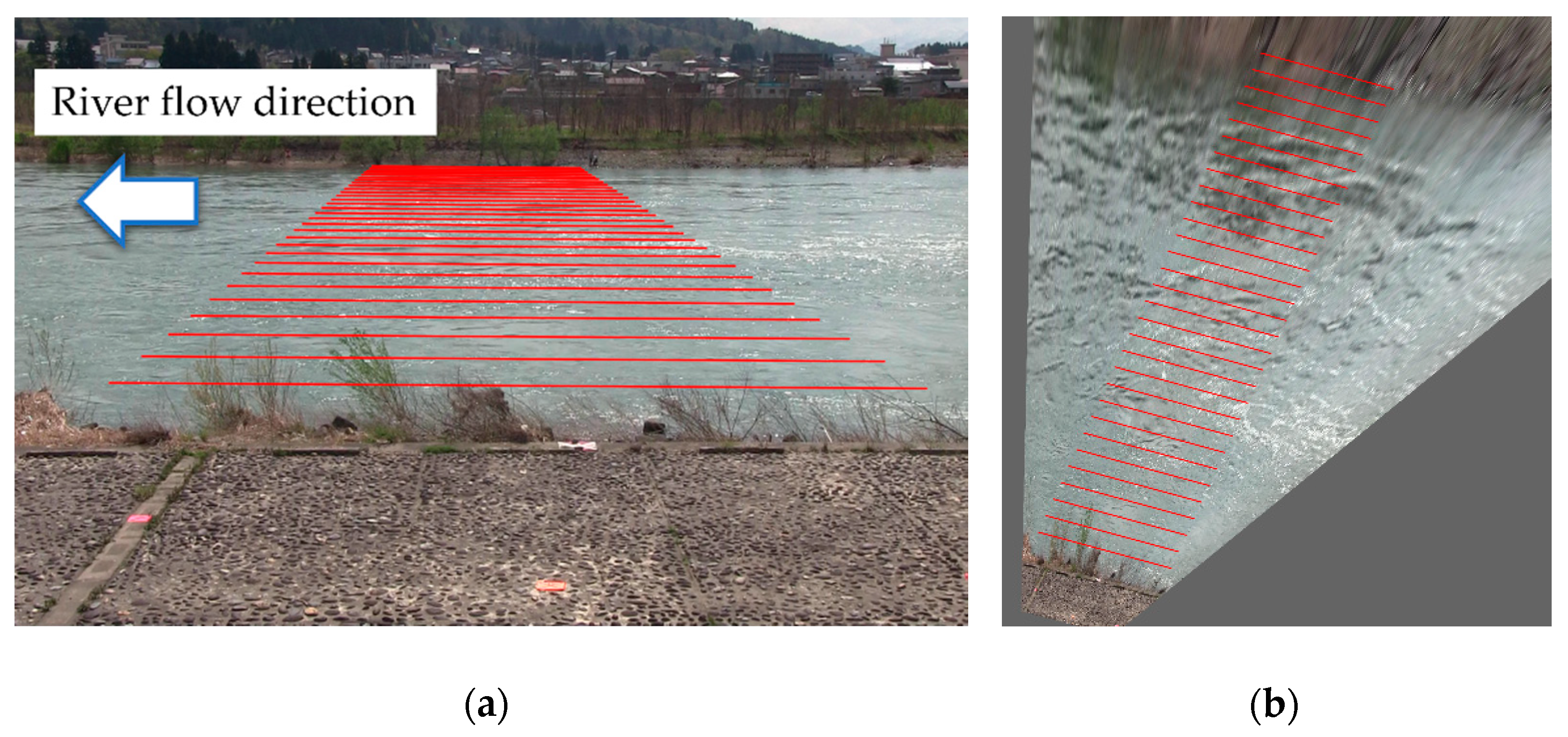
2.1. Image Analysis Procedure of STIV

STIV is an image analysis method for estimating surface velocities in the flow direction by analyzing videos usually taken obliquely from the riverbank as shown in Figure 1a [25,26]. First, search lines with a constant physical length are usually set parallel to the flow direction at regular intervals on the orthorectified image, as shown in Figure 1b. Next, a space-time image (STI) is generated for each search line by stacking the sequential image intensity distribution over time along the search line. As a result, the STI displays inclined patterns indicating the streamwise surface flow velocity at the search line location.
Figure 2 shows an example of the original STI and its two-dimensional Fourier transform image. From the gradient ϕ of the stripe pattern appearing in the STI as the trajectory of the ripples, the flow velocity v is obtained by the following equation with the proportional coefficient k which indicates the conversion between pixels and real scale.
v = k tan ϕ
In recent research, it has been recognized from field observations [28] and direct numerical simulation (DNS) [29] that STI contains textures generated by turbulence-generated ripples advected with the surface velocity, which corresponds to the flow (flow signal), and dispersive wave components traveling in positive or negative directions. As an example, an STI obtained from a river flow movie is shown in Figure 2a, in which textures with different gradients are superposed, which makes the detection of the actual pattern for the surface flow difficult. On the other hand, the Fourier transform image of the STI shown in Figure 2b clearly demonstrates the differences between each component as different locations in the image. Since the linear texture passing through the origin corresponds to the flow signal component, it is useful to use the Fourier transform image to determine the pattern gradient corresponding to the average surface velocity over the search line and measurement time. As described above, the STI texture contains various patterns generated not only by turbulence-related ripples but also by the effects of dispersive waves propagating in all directions, as well as various types of noise generated by other causes. Therefore, the measurement accuracy of STIV depends on how accurately it can detect the texture pattern gradients associated with only the surface flow signals.

2.2. Conventional STIV Methods

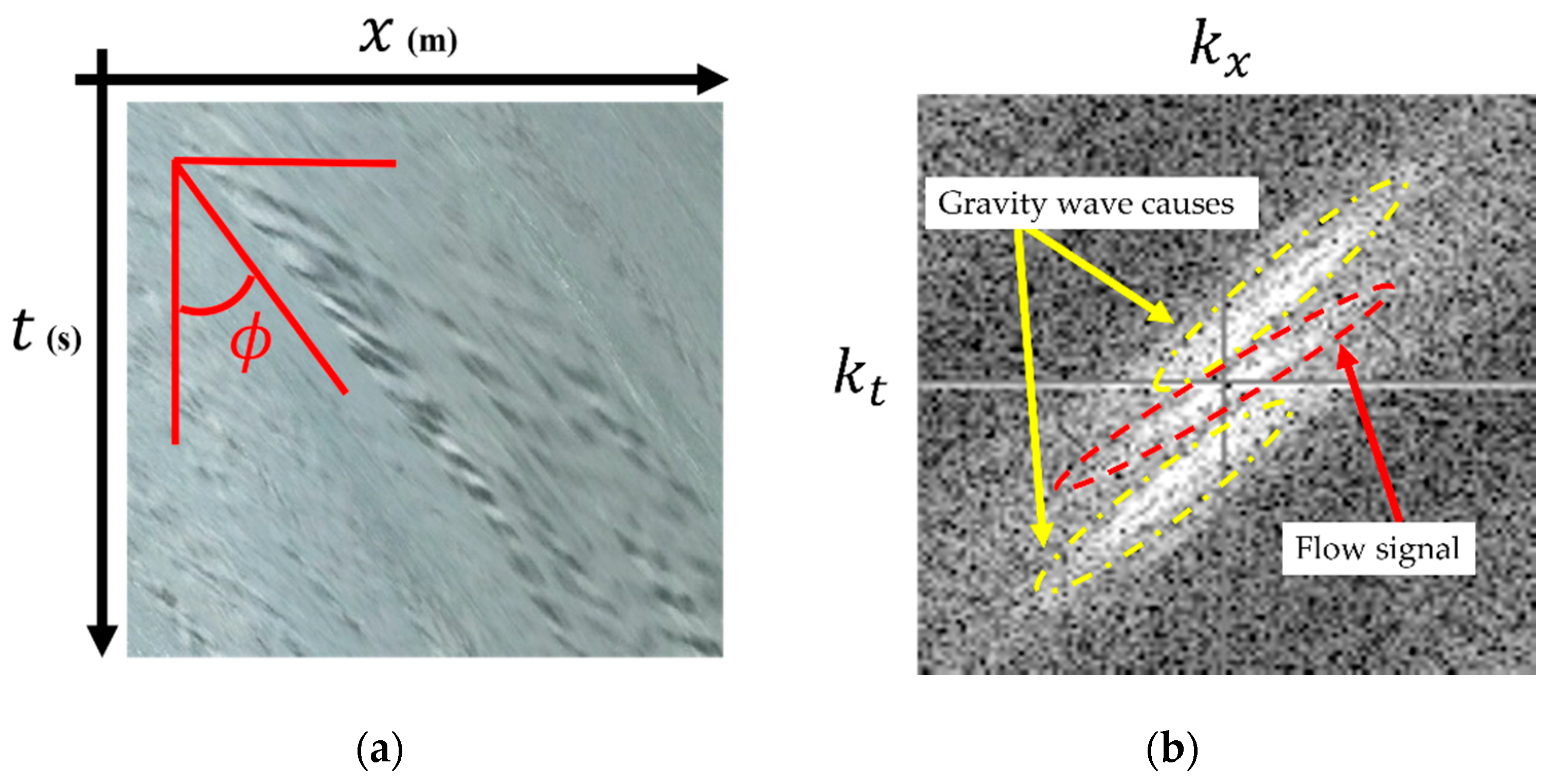
2.2.1. Gradient Tensor Method

This method calculates the gradient tensor of an STI and performs a pattern angle estimation [19]. The method consists of the following steps. First, the STI is divided into a number of overlapping blocks (windows), and the pattern angle is calculated for each block using Equations (2) and (3) (Figure 3a). g ( x ,   t ) in Equation (3) is the image intensity value of the STI image at ( x ,   t ) . p and q take either x or t .
tan 2 ϕ = 2 J x t J t t J x x
J p q = W i n d o w g ( x , t ) p g ( x , t ) q d x d t
Next, the coherency (pattern clarity) of each block is calculated using Equation (4) (Figure 3b).
C = ( J t t J x x ) 2 + 4 J x t 2 J x x + J t t
Finally, a histogram of the pattern angles calculated in the first step is created (Figure 3c), and the average angle weighted by the coherency using Equation (5) is calculated, where N is the number of blocks.
ϕ ¯ = i = 1 N C ( i ) ϕ ( i ) i = 1 N C ( i )
This is the first automatic estimation method developed in STIV, and it can accurately estimate the pattern angle for videos with good shooting conditions. On the other hand, for videos shot under bad conditions, delicate adjustment of parameters such as window size ( M X ,   M T ), window step width ( L X ,   L T ), coherency threshold ( C T ), and histogram range to be averaged ( H R ) is required for a reasonable analysis. In this study, these parameters were set as follows: ( M X ,   M T ) = (30 pix, 30 pix), ( L X ,   L T ) = (10 pix, 10 pix), C T = 0.0, and H R was set to a range up to 70% of the maximum value, which gives reasonable results in many usual cases.

2.2.2. Fourier Predominant Angular Analysis Method

This method uses Equation (6) to calculate the integral of the radial intensities of each angle in the STI’s Fourier transform image and uses the angle with the largest integral value as the pattern angle of the STI (Figure 4).
I ( θ ) = G ( θ ,   r ) d r
Here, G ( θ ,   r ) is the intensity value of the Fourier transform image at ( θ ,   r ) in polar coordinate. The reason this works is because, as mentioned above, the flow signal pattern shows a linear peak through the origin of the STI’s Fourier transform image. Note that the peak angle θ appearing in the Fourier transform image and the gradient angle of the original STI stripe pattern ϕ have an orthogonal relationship. Although fast and robust angle estimation is possible in many cases, these peak structures appearing in the Fourier transform image may be mis-detected in cases where stationary noise and gravity waves are dominant. Furthermore, in the case of strong blur, the peak structure does not appear clearly, and the analysis value may fluctuate greatly depending on the high-pass filter range in the Fourier transform image which is applied as pre-processing. Therefore, in previous research [21,26], the maximum angle is not directly adopted, but is used as filter before the execution of the gradient tensor method. In this study, the high-pass filter applied as pre-processing was set to 1% of the STI size, which gives reasonable results in many usual cases.

3. Automatic Detection of STI Pattern Gradients by Deep Learning

3.1. Outline of Deep Learning

Starting with the success of AlexNet [30] in the ImageNet Large Scale Visual Recognition Challenge (ILSVRC) in 2012, research and development of deep learning methods for various image analysis tasks have been vigorously pursued in recent years. In particular, the development of a convolutional neural network (CNN) has been remarkable in image analysis tasks. CNN is based on a multilayered structure consisting of a convolutional layer extracting image features and a pooling layer that compresses the extracted features. For details, refer to references [30,31,32,33,34].

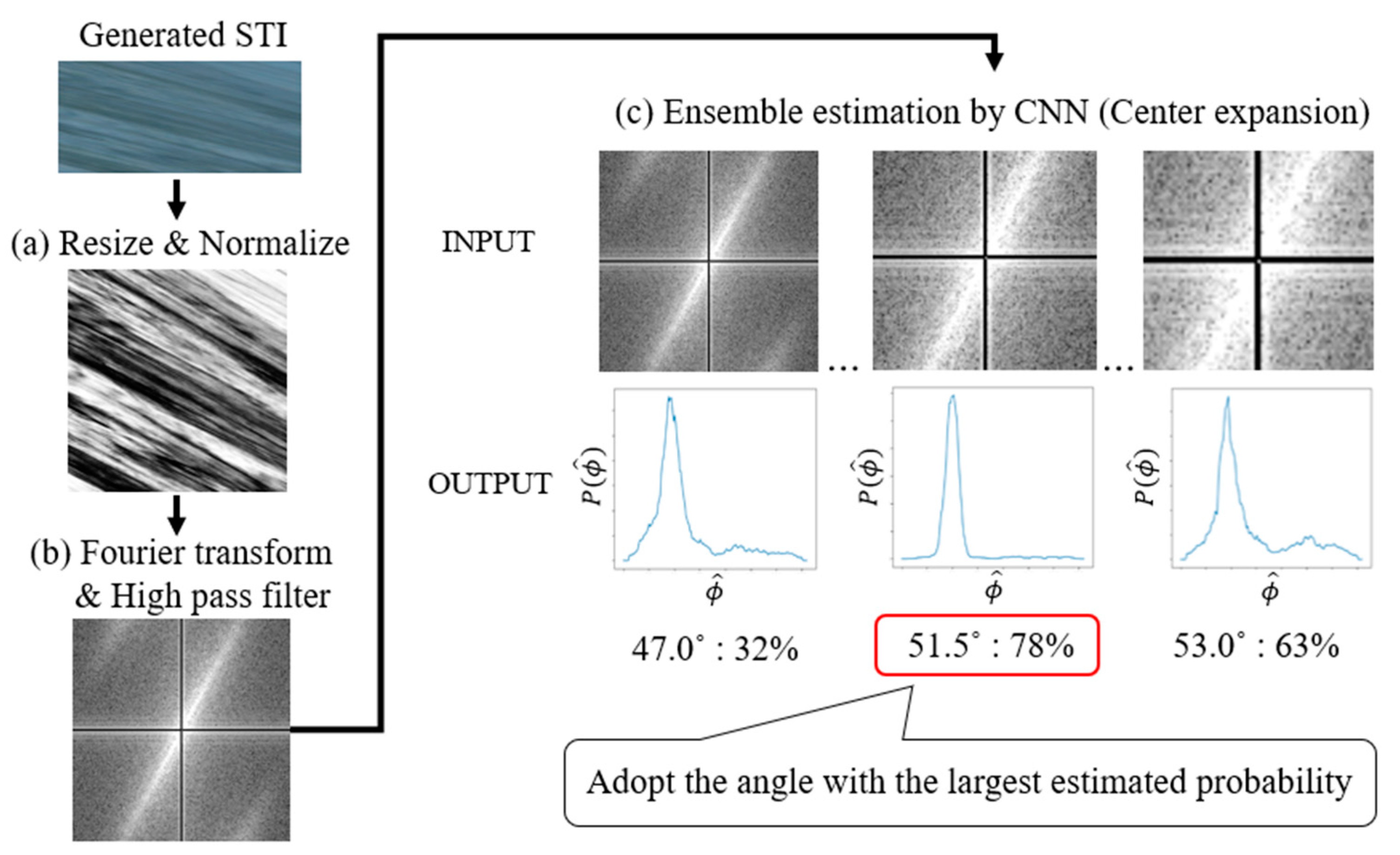
3.2. Application of CNN to a STI Pattern Gradient Detection Problem

In STIV, the flow velocity v is obtained by Equation (1) with the gradient ϕ of the stripe pattern appearing in the STI. Hence, the automatic detection of STI pattern gradients is achieved by using a CNN to accurately approximate the following nonlinear function f ( I ) , which calculates the gradient ϕ of the stripe pattern from the STI information I C h × H × W .   C h is the number of the STI channels, corresponding to 3 for an RGB image and 1 for a grayscale image, H is the height of the STI, indicating the number of image frames that make up the STI, and W is the width of the STI, which is the number of pixels that make up the search line.
ϕ = f ( I )
In the CNN approximation of f ( I ) , it is natural to train it as a regression problem to output the correct pattern gradient value for the input STI. However, in this study, we classify the range from 0° to 180° into N classes with a specific incremental range and train the CNN as a classification problem to estimate the corresponding gradient class from the input STI. In other words, we used CNN to approximate the pattern gradients classification probability distribution p when image intensity value information I is given as shown in the following equation, and the estimated gradient ϕ is ϕ ^ { ϕ 1 ,   ϕ 2 ,   · · · ,   ϕ N } which gives the maximum probability.
ϕ = argmax   ϕ ^ p ( ϕ ^   | I )
This allows not only estimation of gradient values, but also output of estimated probability distributions belonging to each class, confidence interval evaluation of estimated gradient values, and ensemble estimation. By applying multiple pretreatment methods, the highest gradient is adopted from the classification probability (confidence level) of each STI. Furthermore, we use the two-dimensional Fourier transform image [35] of the STI as input to the CNN instead of the original STI because, as described in Section 2.1, the Fourier transform image makes it easier to identify the pattern gradient corresponding to the average surface velocity.
Figure 5 shows the process of pattern gradient detection by CNN. First, the STI generated from the search line is resized and normalized (Figure 5a). Next, a 2D Fourier transformation is performed and a high-pass filter is applied to remove static components such as obstacles (Figure 5b). The preprocessed image is input into the CNN and the classification probability distribution of the pattern gradient is output as a result. Ensemble estimation is performed using multiple images with the center of the image magnified, taking into account that the pattern gradient due to the surface features generated by the turbulence corresponds to the surface average velocity passing through the origin (Figure 5c). Finally, the velocity value is calculated from Equation (1) by using the estimated gradient ϕ ^   with the maximum probability instead of ϕ .

4. Experiments

4.1. Training the CNN with Synthetic STI Dataset

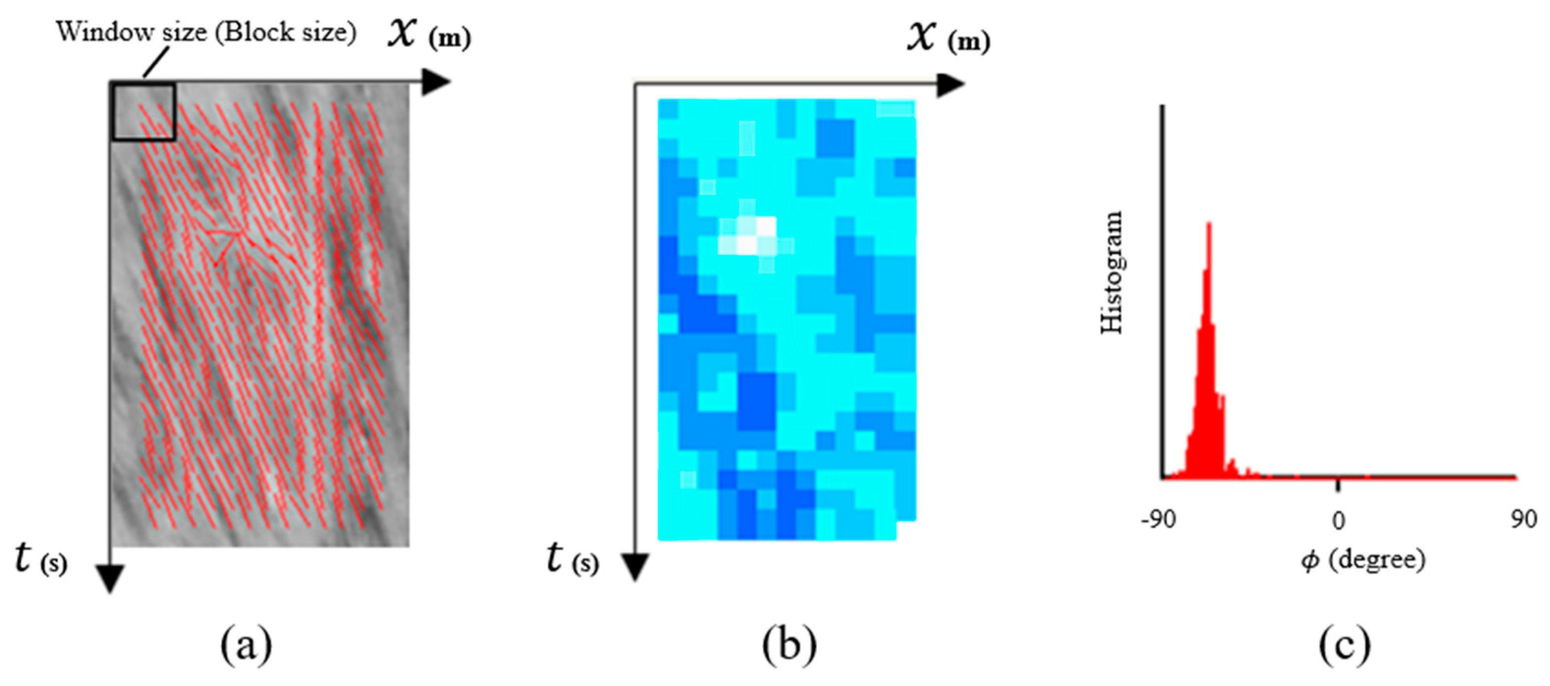
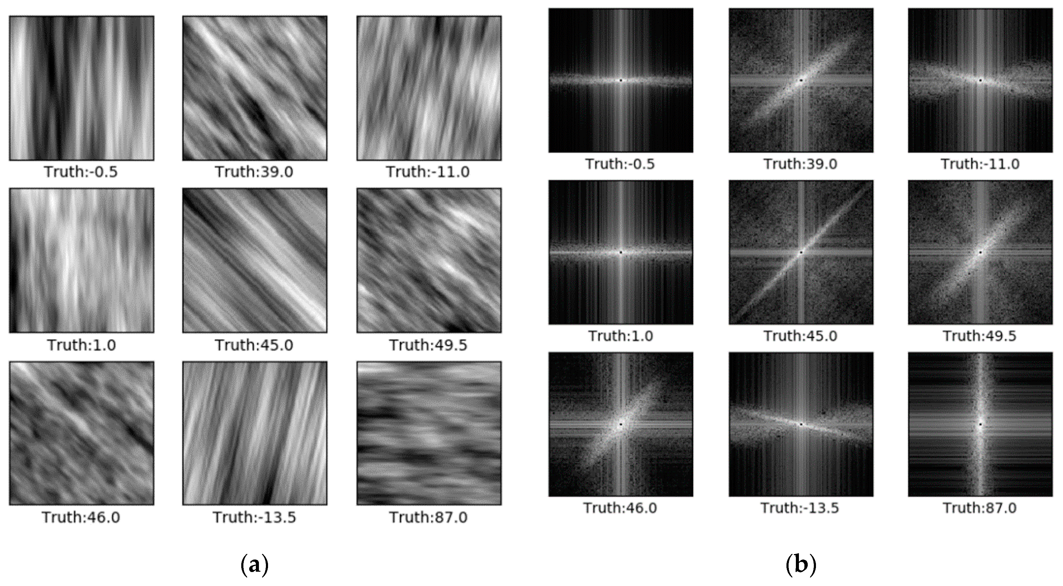
4.1.1. Generation of Synthetic Dataset

For training and validation datasets, Perlin noise-based [36] artificial STI data of size 128 × 128 were generated. Specifically, 300 base images were generated by weighting and averaging the pixel values of three to five stripe pattern images. The images were generated by randomly selecting the number of nodes for setting the gradient with Perlin noise from the range of 2–48. To obtain the STI with various image intensity distributions, 100 images were randomly selected from these base images, rotated by selecting the rotation angle from the normal distribution where the variance σ from the target angle was 1.5°, and then normalized after the weighted average of pixel values to obtain the final artificial STI (Figure 6). The dataset consists of a pair of Fourier transform images of each artificial STI and the corresponding gradient angle (correct label). Since the artificial STI is square, the peak angle of the Fourier transform image and the gradient angle of the original STI stripe pattern are orthogonal. The dataset is divided into 360 classes from 0° to 180° in 0.5° increments. Each class contains 100 images for training and 10 images for accuracy verification. The total amount of data in the dataset is 360 × 100 = 36,000 training pairs and 360 × 10 = 3600 images for accuracy verification.

4.1.2. Deep Neural Network Structure and Learning Configurations

In this study, we adopted a network structure that applies GAP (Global Average Pooling) [31] to multilayer CNNs. This network structure has been used in many image classifications tasks, and the GAP layer, which is placed at the final layer of the multilayer CNN feature extraction, compresses the two-dimensional information of each channel into scalar values to reduce the weight of the model and prevent overfitting. The learning conditions are listed in Table 1 and the network parameters after tuning are shown in Table 2. The input is a Fourier transform image of STI resized to 128 × 128 pixels after gray scaling, and the output is a 360-class classification probability distribution divided into classes between 0°–180° in 0.5° increments. As shown in Equation (1), tan ϕ and   k are used to convert the angle into velocity, so even if the angular resolution is the same, the larger the ϕ and k , the lower the velocity resolution. For example, for a flow velocity of 1.0 m/s at 45°, the resolution is 1.0 ±   0.017 m/s, and for a flow velocity of 1.0 m/s at 70°, the resolution is 1.0 ± 0.028 m/s, which is sufficient for practical use. “Conv” is the Convolution layer, “MaxPool” is the MaxPooling layer, “Dropout” is the Dropout layer, and “Dense” is the Full connected layer (the number of cells is 360, the same as the number of classes). “Res I/O” and “Ch I/O” indicate how the size of the input data and the number of channels is converted in each layer. “Kernel” is the kernel size (filter size) in the Convolution and MaxPooling layers. As the activation function, Leaky-ReLU is used in the Convolution layer and the softmax function is used in the Full connected layer.

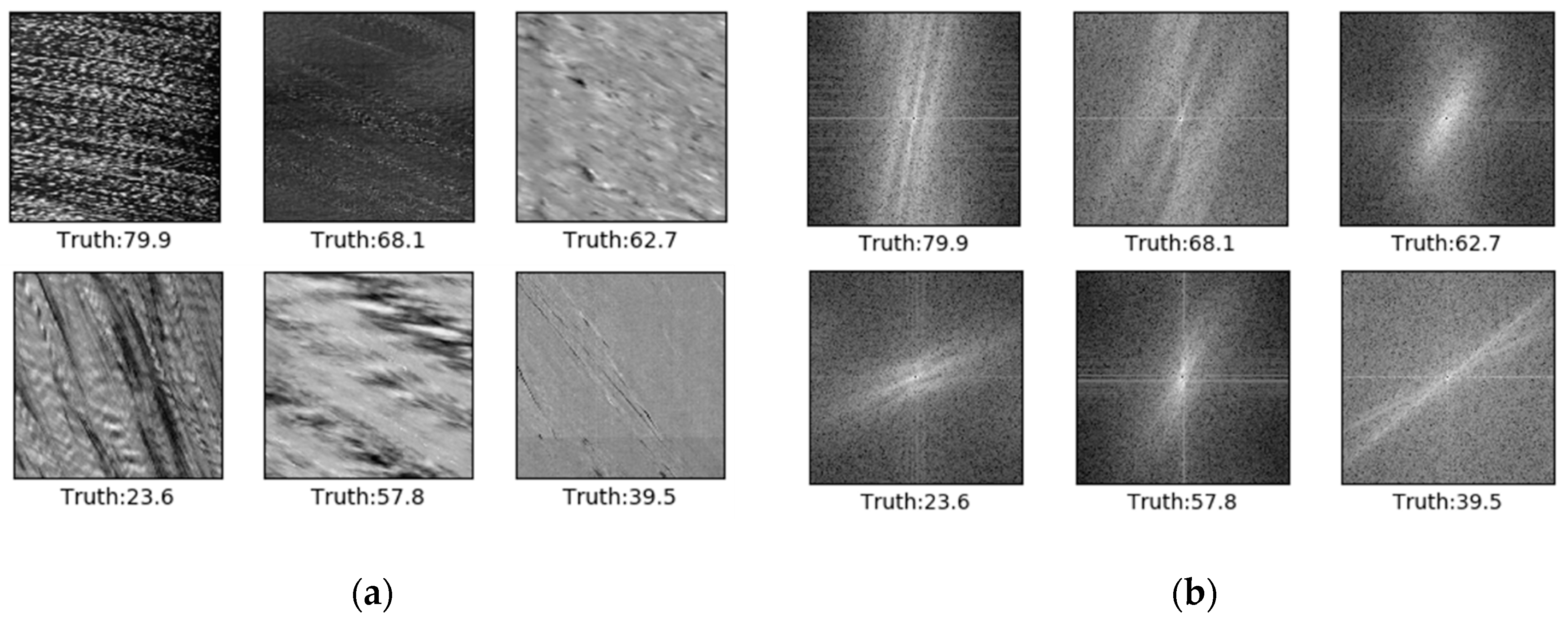
4.2. Application to Synthetic STI Dataset

The results of the application to artificial STI (mentioned in Section 4.1.1 as 3600 images for accuracy verification) are shown in Figure 7 (the red line in the figure is the CNN estimated angle). As mentioned earlier, if we keep in mind that the peak angle appearing in the Fourier transform image and the gradient angle of the stripe pattern in the original STI have an orthogonal relationship, we can confirm that good identification accuracy is shown. Reflecting the fact that the training data generation was performed in the normal distribution range where the variance σ from the target angle was 1.5, we confirmed that the identification accuracy was close to 99% in the range of ± 1.0° to ± 1.5°, where differences could not be identified visually due to blurring caused by angular variance (Table 3).

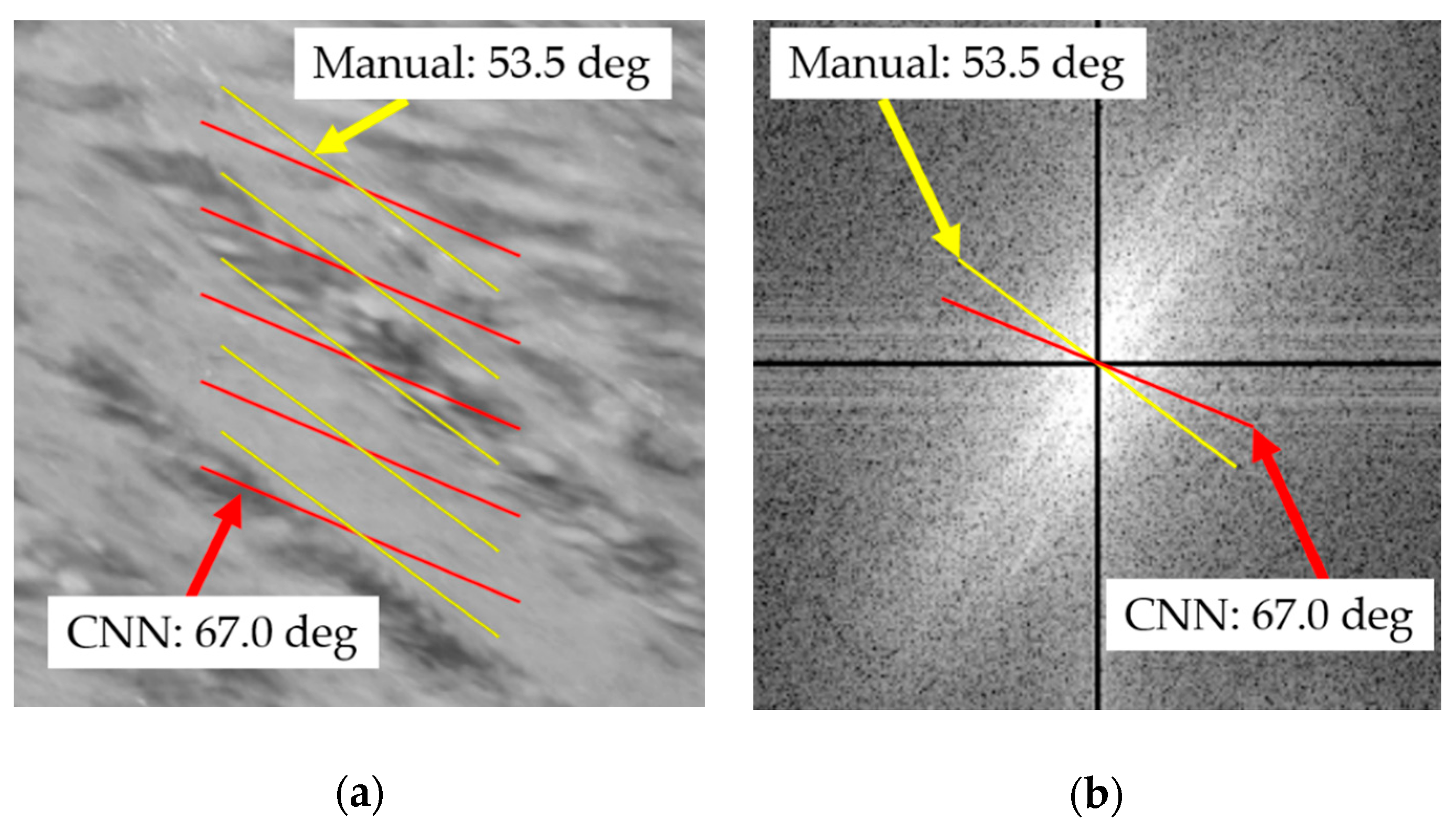
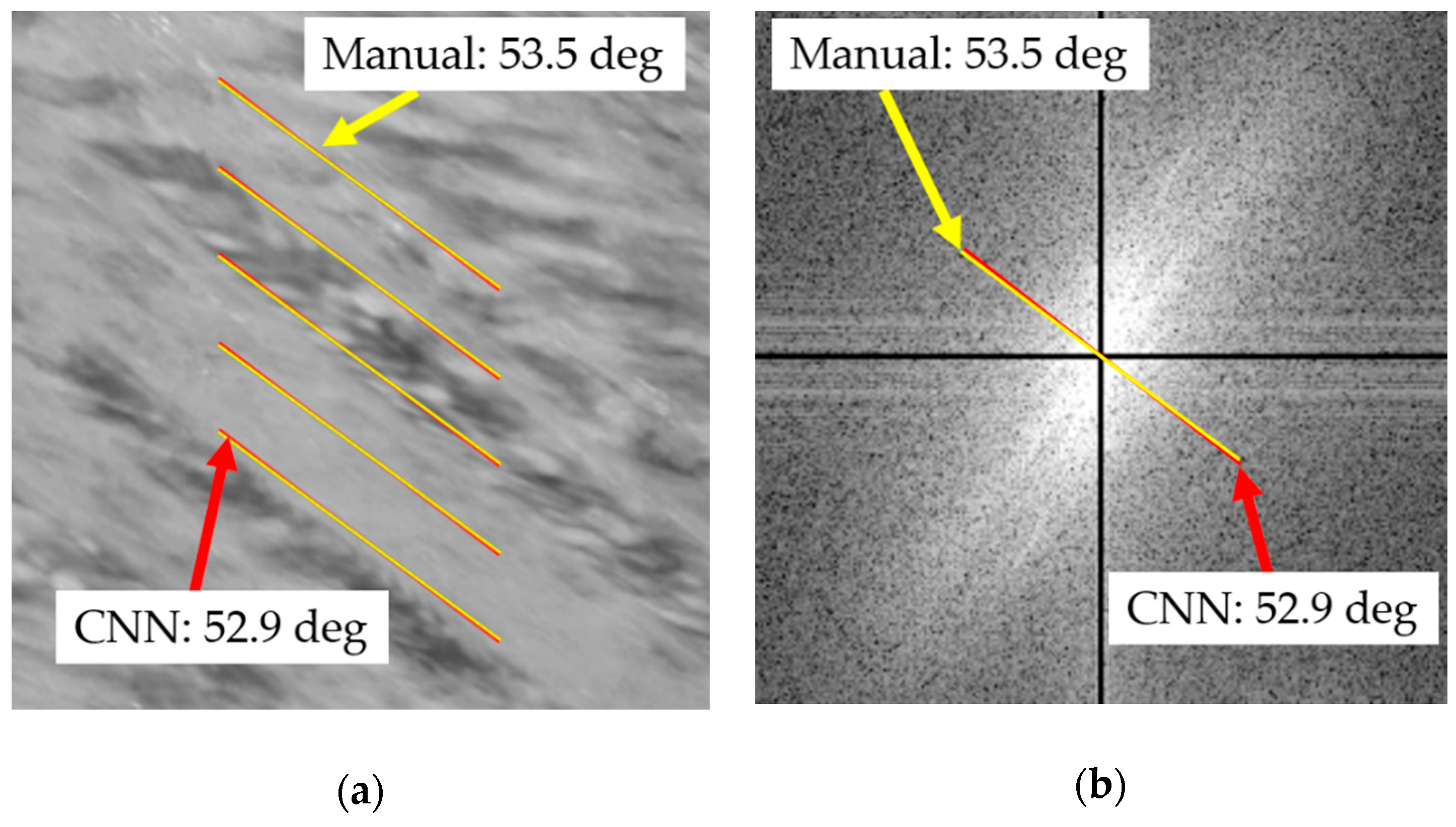
4.3. Application to Categorized STI Dataset

To verify the applicability of the method to STI obtained from real river movies, we applied the method to characteristic STI patterns (Figure 8), which often produce erroneous values in the existing automatic analysis methods. For details on the shooting conditions under which each STI pattern appears, refer to Fujita et al. (2020) [26]. STI patterns that are difficult to detect visually have been excluded from validation for comparison with visual results. The following verification is based on the CNN that trained the artificial STI in the previous section, but since the angular resolution is in increments of 0.5°, the angular resolution was improved by combining the existing method of Fourier predominant angular analysis [26]. Specifically, we performed the Fourier predominant angular analysis with 0.1° angle increments within the range of ± 2.0° of the CNN angle estimate and used the result as the CNN estimate. Figure 9 shows the results of comparing the CNN estimated angle with the conventional automatic analysis method, the gradient tensor method, for the manually confirmed pattern angle. Even with the STI pattern, which is an outlier of the traditional gradient tensor method, the CNN shows good estimation accuracy of about ±3° (black dotted line in Figure 9). As mentioned earlier, the accuracy of the velocity depends on   ϕ and k , but within ± 3°, the error range is at most 10 to 15% of the velocity value in most cases.

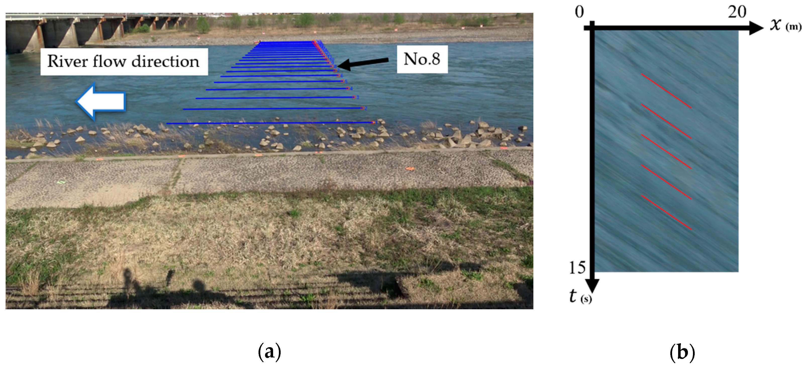
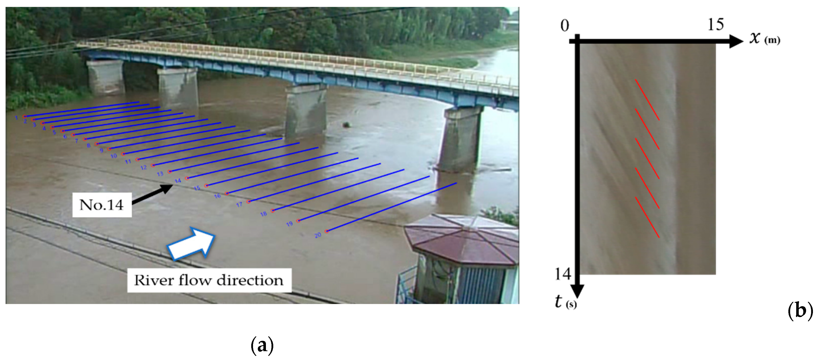
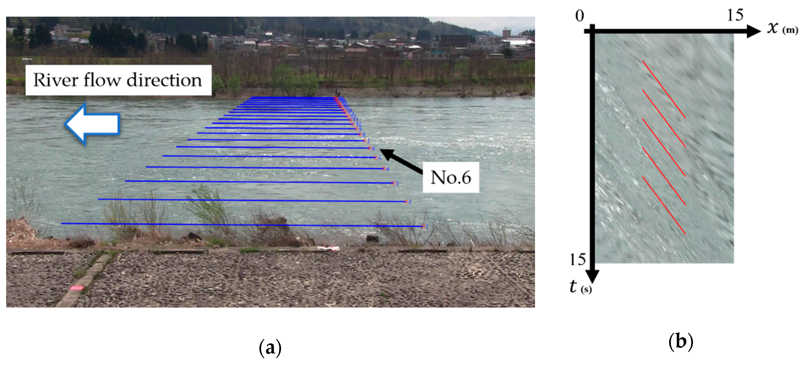
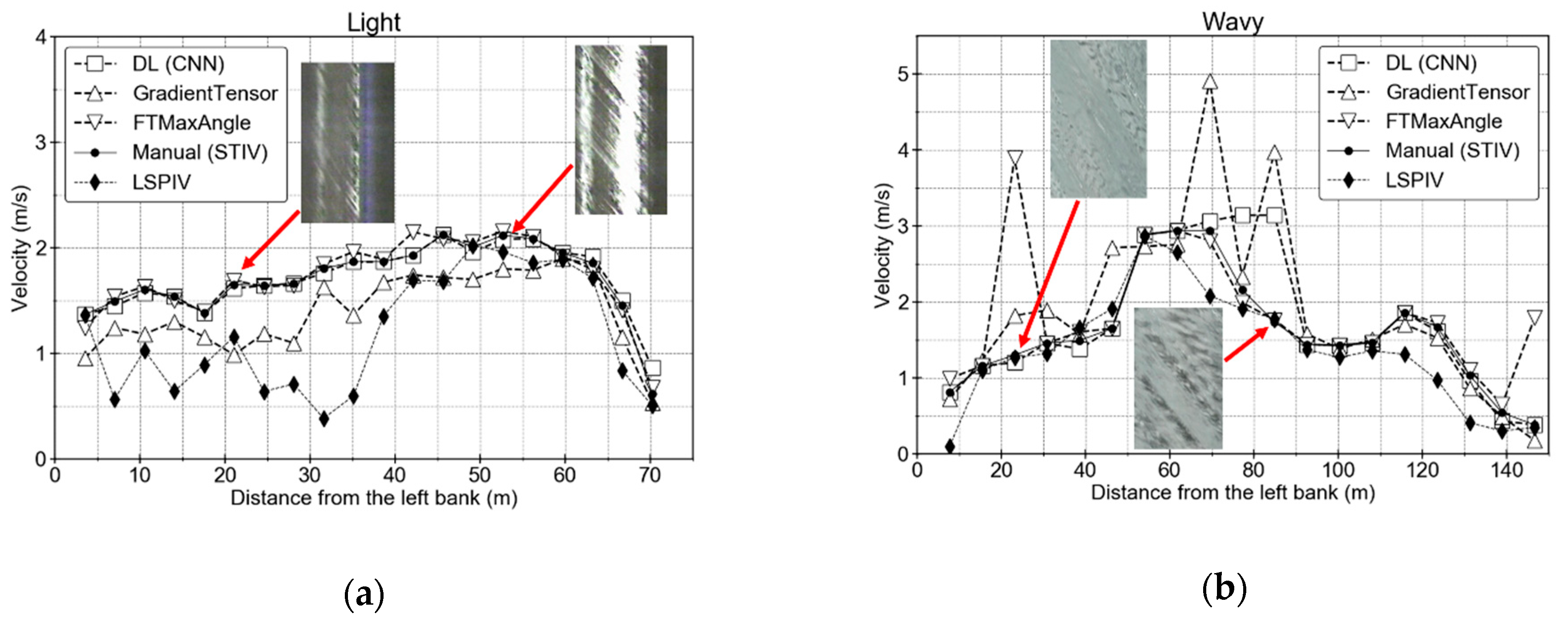
4.4. Application to River Flow Measurement

To verify the applicability of the method to real-time measurements in a real river, we compared the results of the CNN estimation (combined with the Fourier superior angle analysis) described in the previous section with the results of the conventional gradient tensor method, the Fourier predominant angular analysis method (FTMaxAngle), manual analysis, and LSPIV analysis using Fudaa-LSPIV software (Version 1.7.3, which is available as free software from EDF and Irstea, Paris, France.) [37,38]. Assuming a real-time measurement system, the conventional STIV method used all common parameters (parameter values are described in Section 2.2) and did not adjust the parameters on a case-by-case basis. On the other hand, in the LSPIV analysis, the parameters had to be adjusted for each case because it is difficult to analyze various cases with common parameters. The details of the settings of the LSPIV analysis are shown in Table 4.
Figure 10, Figure 11, Figure 12 and Figure 13 show the measurement conditions for cases where STI is classified as normal, shadow, light, and wavy, respectively [26]. In the normal case, since the water surface is fairly flat and the flow velocity is nearly constant, the STI exhibits a linear parallel pattern without significant noise. In the shadow case, part of the search line crosses the shaded area created by the bridge, and the STI shows a non-uniform texture. The light case is obtained from nighttime shooting, where the reflection from the streetlight makes part of the STI too bright, making it difficult to detect the texture indicating the flow signal. In the wavy case, the boil vortices are actively interacting with the water surface. In this case, the combination of the dispersive waves caused by the boil vortices and the advection of the water surface features produces a complex pattern on the STI.
Figure 14 and Figure 15 show the analysis results and the root mean square error (RMSE) of each case is summarized in Table 5. When compared with LSPIV, the normal case shows good consistency between STIV and LSPIV. However, in the shadow and light cases, where the videos were taken under unfavorable conditions, the analyzed velocities by LSPIV are unstable and underestimated, especially on the opposite shore side of the camera (left bank side in Figure 14 and Figure 15), where the image resolutions are decreased. In the wavy case, LSPIV also shows good consistency with STIV as in the normal case, but the tendency of underestimation on the opposite shore (right bank side in Figure 15) is the same. These results will be discussed in a later section. As shown in Figure 14 and Figure 15, most of the outliers measured by the conventional STIVs have been improved in the CNN, resulting in robust estimates that are consistent with the manual analysis. However, in the wavy case, there are some STIs where CNN estimates are different from those by the manual estimation. An example of such a case is shown in Figure 16, in which linear peaks due to gravitational waves appear. These patterns are similar to those produced by turbulence (flow signal), but with different coexisting slopes. In such cases, these peaks can be mistaken as a flow signal that corresponds to the average flow velocity on the surface. This is because the training data artificially generated by Perlin noise did not include these patterns.
To improve the false detection case, 500 STIs showing a pattern similar to the false detection case were collected from the actual river video, and additional learning of CNN was performed. Figure 17 shows examples of STIs for additional training data. Angles that can be manually confirmed were set for the labels (ground truths). Since the amount of additional learning data is considerably smaller than the STI artificially generated by Perlin noise: 36,000, the learning utilization ratio of the artificial STI and the STI additionally collected from the actual river video was set to 4:1 by random sampling with duplication. Figure 18 shows the results of re-estimation with the CNN after additional learning for the false detection cases indicated in Figure 16. From Figure 18, it is obvious that the estimated result is greatly improved by additionally learning the cases where multiple peaks coexist in STI.

5. Discussions

In the adverse case shown in Figure 13 and Figure 14, the STIV method using CNN was shown to be stable without any parameter adjustment. Comparing with the results from LSPIV in these cases, the robust measurement performance of STIV is well demonstrated. On the other hand, there are some recent studies concerning the uncertainty introduced in the image velocimetry methods due to adverse conditions, especially in PIV-based methods [39,40]. The parameter sensitivity control method and the velocity correction method proposed in these studies may stabilize and improve the LSPIV results better than the present LSPIV cases, but further examination is necessary. However, as far as the streamwise flow measurement for discharge estimation is concerned, the proposed STIV technique yielded more favorable results than the conventional LSPIV technique. As shown in Figure 16, Figure 17 and Figure 18, although machine learning methods such as deep learning are vulnerable to unlearned patterns, one of the major advantages of the methods is that the accuracy can be continuously improved by learning additional data. As data are accumulated through continuous observation, further improvements in accuracy can be expected by enriching more data to learn in the future. In addition, there is also a possibility of building a CNN that is automatically optimized for each observation point by learning the patterns unique to each point. As for the calculation speed, the CNN took about 0.5-1 s per STI on a consumer-level computer (it requires a CPU that supports the AVX instruction set, but most recent CPUs meet the requirements) to estimate an angle after learning. While not as fast as the gradient tensor method or the Fourier predominant angular analysis method (less than 0.1 s per STI), this is fast enough to build a real-time measurement system, since the measurement frequency in a typical real-time measurement system is about every 10 min to an hour. The most time-consuming part of the STIV process is the STI generation process (less than 10 s per STI in most cases for a 15-s video with 30 fps), and the total time for STIV measurement is less than 1 to 2 min in most cases. Finally, although it might be difficult to make a direct comparison, LSPIV took about 10 times longer than STIV in the present analysis.

6. Conclusions

In this study, we applied a deep learning method to STIV’s STI pattern gradient detection process and verified its effectiveness in realizing a real-time measurement system using STIV. It was confirmed that the new method can provide favorable flow velocity estimations with no parameter adjustment even when the conventional methods yield erroneous results and manual adjustment is required. Unlike conventional methods, the new method has the advantage of being able to continuously improve accuracy by learning from further examples as training data. Although the deep learning method takes time to learn the data, the inference calculation speed in the actual operation after learning is fast, and it is very suitable for real-time measurement systems.

Author Contributions

All authors were involved in study design and data interpretation; I.F. and K.W. wrote the manuscript; I.F. collected measurement data; K.W. developed the software and analyze the data; M.I. and M.H. contributed to the study coordination and the revision of the manuscript. All authors have read and agreed to the published version of the manuscript.

Funding

This research received no external funding.

Institutional Review Board Statement

Not applicable.

Informed Consent Statement

Not applicable.

Acknowledgments

The authors are grateful to the consulting companies in Japan who provided us various types of river surface images under favorable and unfavorable image shooting conditions.

Conflicts of Interest

The authors declare no conflict of interest.

References

  1. Shakti, P.C.; Nakatani, T.; Misumi, R. Hydrological Simulation of Small River Basins in Northern Kyushu, Japan, during the Extreme Rainfall Event of July 5–6, 2017. J. Disaster Res. 2018, 13, 396–409. [Google Scholar] [CrossRef]
  2. Tominaga, A. Lessons Learned from Tokai Heavy Rainfall. J. Disaster Res. 2007, 2, 50–53. [Google Scholar] [CrossRef]
  3. Kazama, M.; Yamakawa, Y.; Yamaguchi, A.; Yamada, S.; Kamura, A.; Hino, T.; Moriguchi, S. Disaster report on geotechnical damage in Miyagi Prefecture, Japan caused by Typhoon Hagibis in 2019. Soils Found. 2021, 61, 549–565. [Google Scholar] [CrossRef]
  4. Nihei, Y.; Sakai, T. ADCP measurements of vertical flow structure and coefficients of float in flood flows. In Proceedings of the 32nd Congress of the International Association of Hydraulic Engineering and Research, Venice, Italy, 1–6 July 2007. [Google Scholar]
  5. Harada, Y.; Nihei, Y.; Sakai, T.; Kimizu, A. Fundamental study on measuring accuracy for flood discharge with floats. Annu. J. Hydraul. Eng. 2007, 51, 1081–1086. (In Japanese) [Google Scholar] [CrossRef] [Green Version]
  6. The Innovative River Technology Project led by the Ministry of Land, Infrastructure, Transport and Tourism (MLIT) in Japan. Available online: https://www.mlit.go.jp/river/gijutsu/inovative_project/project4.html (accessed on 25 June 2021). (In Japanese).
  7. Muste, M.; Yu, K.; Spasojevic, M. Practical aspects of ADCP data use for quantification of mean river flow characteristics; Part I: Moving-vessel measurements. Flow Meas. Instrum. 2004, 15, 1–16. [Google Scholar] [CrossRef]
  8. Muste, M.; Yu, K.; Pratt, T.; Abraham, D. Practical aspects of ADCP data use for quantification of mean river flow characteristics; Part II: Fixed-vessel measurements. Flow Meas. Instrum. 2004, 15, 17–28. [Google Scholar] [CrossRef]
  9. Oberg, K.; Mueller, D.S. Validation of Streamflow Measurements Made with Acoustic Doppler Current Profilers. J. Hydraul. Eng. 2007, 133, 1421–1432. [Google Scholar] [CrossRef] [Green Version]
  10. Yamaguchi, T.; Niizato, K. Flood discharge observation using radio current meter. Proc. Jpn. Soc. Civ. Eng. 1994, 497, 41–50. (In Japanese) [Google Scholar]
  11. Welber, M.; Le Coz, J.; Laronne, J.B.; Zolezzi, G.; Zamler, D.; Dramais, G.; Hauet, A.; Salvaro, M. Field assessment of noncontact stream gauging using portable surface velocity radars (SVR). Water Resour. Res. 2016, 52, 1108–1126. [Google Scholar] [CrossRef] [Green Version]
  12. Muste, M.; Fujita, I.; Hauet, A. Large-scale particle image velocimetry for measurements in riverine environments. Water Resour. Res. 2008, 44, 1–14. [Google Scholar] [CrossRef] [Green Version]
  13. Fujita, I. Discharge Measurements of Snowmelt Flood by Space-Time Image Velocimetry during the Night Using Far-Infrared Camera. Water. 2017, 9, 269. [Google Scholar] [CrossRef]
  14. Hauet, A.; Creutin, J.-D.; Belleudy, P. Sensitivity study of large-scale particle image velocimetry measurement of river discharge using numerical simulation. J. Hydrol. 2008, 349, 178–190. [Google Scholar] [CrossRef]
  15. Fujita, I.; Kawamura, Y. Discharge Measurements of Flood Flow by Imaging Technology and Float Method. In Proceedings of the 29th Congress of IAHR, Beijing, China, 16–21 September 2001; Volume 1, pp. 1–6. [Google Scholar]
  16. Fujita, I.; Muste, M.; Kruger, A. Large-scale particle image velocimetry for flow analysis in hydraulic engineering applications. J. Hydraul. Res. 1998, 36, 397–414. [Google Scholar] [CrossRef]
  17. Muste, M.; Hauet, A.; Fujita, I.; Legout, C.; Ho, H.-C. Capabilities of Large-scale Particle Image Velocimetry to characterize shallow free-surface flows. Adv. Water Resour. 2014, 70, 160–171. [Google Scholar] [CrossRef]
  18. Khalid, M.; Pénard, L.; Mémin, E. Optical flow for image-based river velocity estimation. Flow Meas. Instrum. 2019, 65, 110–121. [Google Scholar] [CrossRef] [Green Version]
  19. Fujita, I.; Watanabe, H.; Tsubaki, R. Development of a non-intrusive and efficient flow monitoring technique: The space-time image velocimetry (STIV). Int. J. River Basin Manag. 2007, 5, 105–114. [Google Scholar] [CrossRef] [Green Version]
  20. Fujita, I.; Kumano, G.; Asami, K. Evaluation of 2D river flow simulation with the aid of image-based field velocity measurement techniques. River Flow. 2014, 1969–1977. [Google Scholar] [CrossRef]
  21. Zhao, H.; Chen, H.; Liu, B.; Liu, W.; Xu, C.-Y.; Guo, S.; Wang, J. An improvement of the Space-Time Image Velocimetry combined with a new denoising method for estimating river discharge. Flow Meas. Instrum. 2021, 77, 101864. [Google Scholar] [CrossRef]
  22. Al-Mamari, M.; Kantoush, S.; Kobayashi, S.; Sumi, T.; Saber, M. Real-Time Measurement of Flash-Flood in a Wadi Area by LSPIV and STIV. Hydrology 2019, 6, 27. [Google Scholar] [CrossRef] [Green Version]
  23. Zhen, Z.; Huabao, L.; Yang, Z.; Jian, H. Design and evaluation of an FFT-based space-time image velocimetry (STIV) for time-averaged velocity measurement. In Proceedings of the 14th IEEE International Conference on Electronic Measurement & Instruments (ICEMI), Changsha, China, 1–3 November 2019. [Google Scholar] [CrossRef]
  24. Hydro-STIV. Available online: https://hydrosoken.co.jp/service/hydrostiv.php (accessed on 25 June 2021).
  25. Fujita, I.; Notoya, Y.; Tani, K.; Tateguchi, S. Efficient and accurate estimation of water surface velocity in STIV. Environ. Fluid Mech. 2018, 19, 1363–1378. [Google Scholar] [CrossRef] [Green Version]
  26. Fujita, I.; Shibano, T.; Tani, K. Application of masked two-dimensional Fourier spectra for improving the accuracy of STIV-based river surface flow velocity measurements. Meas. Sci. Technol. 2020, 31, 094015. [Google Scholar] [CrossRef]
  27. Fujita, I.; Deguchi, T.; Doi, K.; Ogino, D.; Notoya, Y.; Tateguchi, S. Development of KU-STIV: Software to measure surface velocity distribution and discharge from river surface images. In Proceedings of the 37th IAHR World Congress, Kuala Lumpur, Malaysia, 13–18 August 2017; pp. 5284–5292. [Google Scholar]
  28. Tani, K.; Fujita, I. Wavenumber-frequency analysis of river surface texture to improve accuracy of image-based velocimetry. E3S Web Conf. 2018, 40, 06012. [Google Scholar] [CrossRef]
  29. Yoshimura, H.; Fujita, I. Investigation of free-surface dynamics in an open-channel flow. J. Hydraul. Res. 2019, 58, 231–247. [Google Scholar] [CrossRef]
  30. Krizhevsky, A.; Sutskever, I.; Hinton, G.E. ImageNet classification with deep convolutional neural networks. Adv. Neural Inf. Process. Syst. 2012, 25, 1097–1105. [Google Scholar] [CrossRef]
  31. Lin, M.; Chen, Q.; Yan, S. Network in network. In Proceedings of the 2nd International Conference on Learning Representations, ICLR, Banff, AB, Canada, 14–16 April 2014. [Google Scholar]
  32. He, K.; Zhang, X.; Ren, S.; Sun, J. Deep Residual Learning for Image Recognition. In Proceedings of the IEEE conference on computer vision and pattern recognition, Las Vegas, NV, USA, 27–30 June 2016. [Google Scholar]
  33. Hu, J.; Shen, L.; Albanie, S.; Sun, G.; Wu, E. Squeeze-and-Excitation Networks. In Proceedings of the IEEE conference on computer vision and pattern recognition, Salt Lake City, UT, USA, 18–22 June 2018. [Google Scholar]
  34. Tan, M.; Le, Q.V. Efficientnet: Rethinking model scaling for convolutional neural networks. In Proceedings of the 36th International Conference on Machine Learning (ICML 2019), Long Beach, CA, USA, 10–15 June 2019. [Google Scholar]
  35. Dolcetti, G.; Horoshenkov, K.; Krynkin, A.; Tait, S.J. Frequency-wavenumber spectrum of the free surface of shallow turbulent flows over a rough boundary. Phys. Fluids. 2016, 28, 105105. [Google Scholar] [CrossRef] [Green Version]
  36. Perlin, K. Improving noise. ACM Trans. Graph. (TOG) 2002, 21, 681–682. [Google Scholar] [CrossRef]
  37. Fudaa-LSPIV. Available online: https://forge.irstea.fr/projects/fudaa-lspiv (accessed on 25 June 2021).
  38. Le Coz, J.; Jodeau, M.; Hauet, A.; Marchand, B.; Le Boursicaud, R. Image-based velocity and discharge measurements in field and laboratory river engineering studies using the free Fudaa-LSPIV software. In Proceedings of the International Conference on Fluvial Hydraulics, River Flow 2014, Lausanne, Switzerland, 3–5 September 2014; pp. 1961–1967. [Google Scholar]
  39. Detert, M. How to Avoid and Correct Biased Riverine Surface Image Velocimetry. Water Resour. Res. 2021, 57, e2020WR027833. [Google Scholar] [CrossRef]
  40. Rozos, E.; Dimitriadis, P.; Mazi, K.; Lykoudis, S.; Koussis, A. On the Uncertainty of the Image Velocimetry Method Parameters. Hydrology 2020, 7, 65. [Google Scholar] [CrossRef]
Figure 1. Original and orthorectified images with search lines: (a) original; (b) orthorectified image.
Water 13 02079 g001
Figure 2. Space-time Image (STI): (a) original image; (b) 2D Fourier transform image.
Water 13 02079 g002
Figure 3. Process of the gradient tensor method: (a) calculated pattern angle with each block; (b) calculated coherency with each block; (c) a histogram of the pattern angles.
Water 13 02079 g003
Figure 4. Process of the Fourier predominant angular analysis method: (a) original STI; (b) 2D Fourier transform image; (c) calculated radial intensity value integral for each angle.
Water 13 02079 g004
Figure 5. Process flow of STI pattern gradient detection by Convolutional Neural Network (CNN): (a) The generated STI is resized and normalized; (b) A 2D Fourier transformation is performed and a high-pass filter is applied; (c) Ensemble CNN estimation is performed using multiple images with the center of the image magnified.
Water 13 02079 g005
Figure 6. Artificial STI generated by Perlin noise. ”Truth” labels indicate designated angles (in degrees): (a) original images; (b) 2D Fourier transform images.
Water 13 02079 g006
Figure 7. Application results for artificial STIs. ”Truth” labels indicate designated (ground truth) angles (in degrees), ”CNN” labels indicate estimated angles (in degrees) by CNN: (a) original images; (b) 2D Fourier transform images.
Water 13 02079 g007
Figure 8. Categorized STIs (red lines are CNN estimated angles).
Water 13 02079 g008
Figure 9. Comparison with manually confirmed angles: (a) CNN; (b) gradient tensor method.
Water 13 02079 g009
Figure 10. Normal case: The water surface is fairly flat and the flow velocity is nearly constant. The STI exhibits a linear parallel pattern without significant noises. (a) Obliquely viewed image; (b) STI, No.8 (red lines are CNN estimated angles).
Water 13 02079 g010
Figure 11. Shadow case: Part of the search line crosses the shaded area created by the bridge. The STI shows a non-uniform texture. (a) Obliquely viewed image; (b) STI, No.14 (red lines are CNN estimated angles).
Water 13 02079 g011
Figure 12. Light case: The nighttime shooting. The reflection from the streetlight makes part of the STI too bright, making it difficult to detect the texture indicating the flow signal. (a) Obliquely viewed image; (b) STI, No.10 (red lines are CNN estimated angles).
Water 13 02079 g012
Figure 13. Wavy case: The boil vortices are actively interacting with the water surface. The combination of the dispersive waves caused by the boil vortices and the advection of the water surface features produces a complex pattern on the STI. (a) Obliquely viewed image; (b) STI, No.6 (red lines are CNN estimated angles).
Water 13 02079 g013
Figure 14. Comparison of cross-sectional flow velocity distributions: (a) normal case; (b) shadow case (STIs on the graph are histogram equalization filtered for visibility).
Water 13 02079 g014
Figure 15. Comparison of cross-sectional flow velocity distributions: (a) light case; (b) wavy case.
Water 13 02079 g015
Figure 16. The false detection of peak angle case (red: CNN estimation, yellow: manual estimation): (a) original image; (b) 2D Fourier transform image.
Water 13 02079 g016
Figure 17. Additional training data collected from real river videos. ”Truth” labels indicate correct (ground truth) angles (in degrees): (a) original images; (b) 2D Fourier transform images.
Water 13 02079 g017
Figure 18. Angle detection results after additional data training (red: CNN estimation, yellow: manual estimation): (a) original image; (b) 2D Fourier transform image.
Water 13 02079 g018
Table 1. The details of the learning conditions.
Setting ItemValue
Loss functionCross entropy
Optimization algorithmAdam
Learning rate0.0001
Number of learning data36,000 (100/class)
Batch size32
Number of learning epoch6
Table 2. The details of the CNN model.
LayerResolution I/OChannel I/OKernel
Conv1128/1281/327 × 7
Conv2128/12832/325 × 5
MaxPool1128/6432/322 × 2
Dropout164/6432/32-
Conv364/6432/645 × 5
Conv464/6464/643 × 3
MaxPool264/3264/642 × 2
Dropout232/3264/64-
Conv532/3264/1285 × 5
Conv632/32128/1283 × 3
MaxPool332/16128/1282 × 2
Dropout316/16128/128-
Conv716/16512/5125 × 5
Conv816/16512/5123 × 3
GAP16/1512/51216 × 16
Dense1/1512/360-
Conv1128/1281/327 × 7
Table 3. Estimation accuracy at each tolerance (correct answer rate).
Tolerance ± 0° ± 0.5° ± 1.0° ± 1.5° ± 2.0°
Accuracy33.0%80.2%97.0%99.5%99.9%
Table 4. The details of the settings of the LSPIV analysis. Velocities were calculated as the average of the velocities of all frames after filtering out those with correlation coefficients less than 0.5.
CaseTime StepOrthorectified Image Pixel ScaleInterrogation Area Size (IA)Search Area Size (SA)
Normal0.2 s0.05 m/pix60 ×   6 0 pix (3 m2)40 pix ( ± 10 m/s)
Shadow0.1 s0.05 m/pix100 × 100 pix (5 m2)20 pix ( ± 10 m/s)
Light0.3 s0.05 m/pix100 × 100 pix (5 m2)30 pix ( ±   5   m/s)
Wavy0.1 s0.05 m/pix60 ×   6 0 pix (3 m2)10 pix ( ±   5   m/s)
Table 5. The root mean square error (RMSE) of each case assuming the results of STIV manual analysis are the correct values. (The LSPIV results are excluded since the comparison is made when the results of STIV manual analysis are taken as the correct values).
CaseDL (CNN)Gradient TensorFTMaxAngle
Normal0.120.120.22
Shadow0.060.391.15
Light0.060.350.07
Wavy0.400.750.68
Publisher’s Note: MDPI stays neutral with regard to jurisdictional claims in published maps and institutional affiliations.

