
Frequency Analysis of Snowmelt Flood Based on GAMLSS Model in Manas River Basin, China


Abstract
:1. Introduction
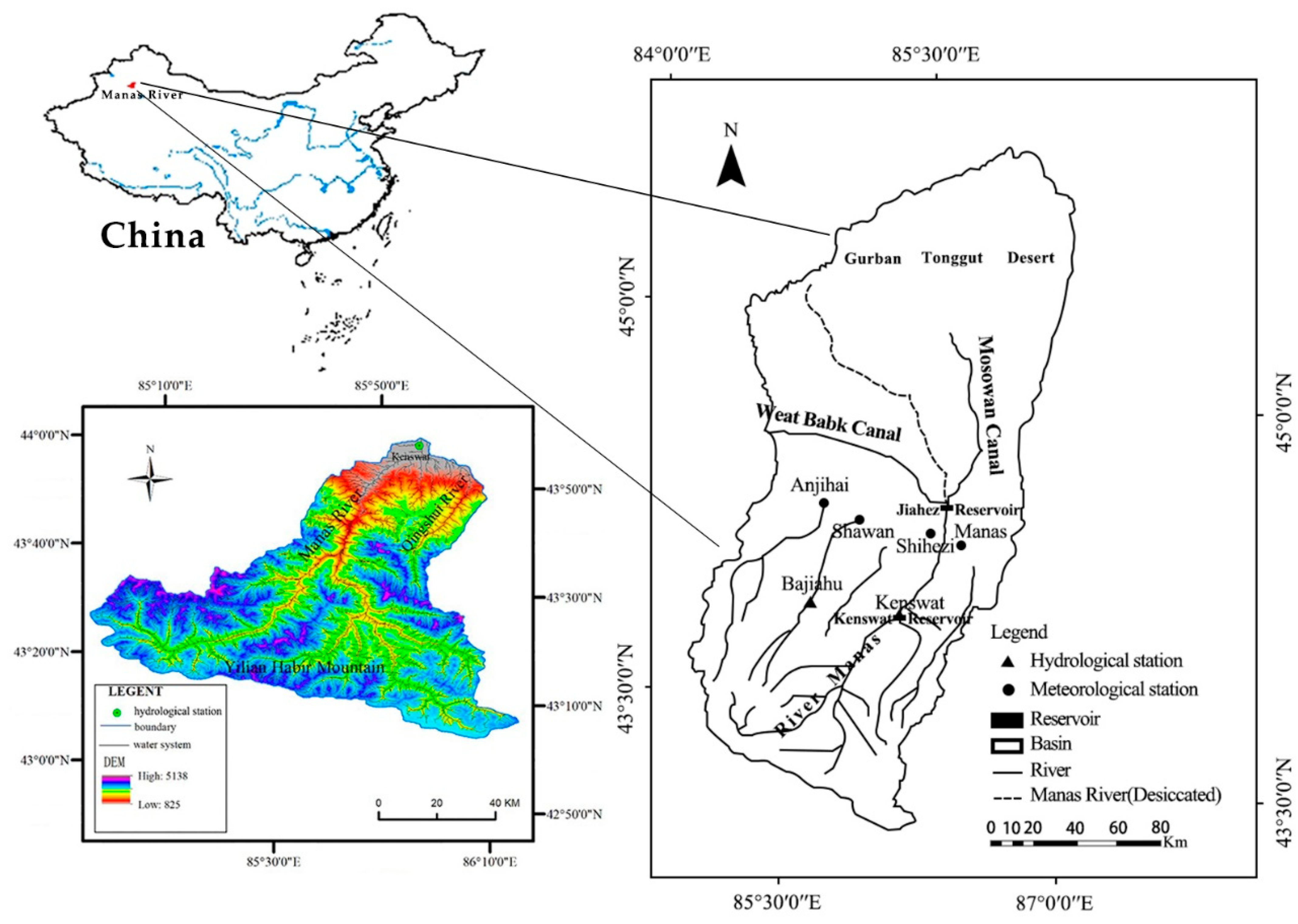
2. Study Area
3. Data and Methods
3.1. Dataset
3.2. Methods
3.2.1. Correlation Analysis
3.2.2. Generalized Additive Models for Location, Scale, and Shape (GAMLSS) Theory
4. Results
4.1. Correlation Analysis of Temperature and Snowmelt Flood
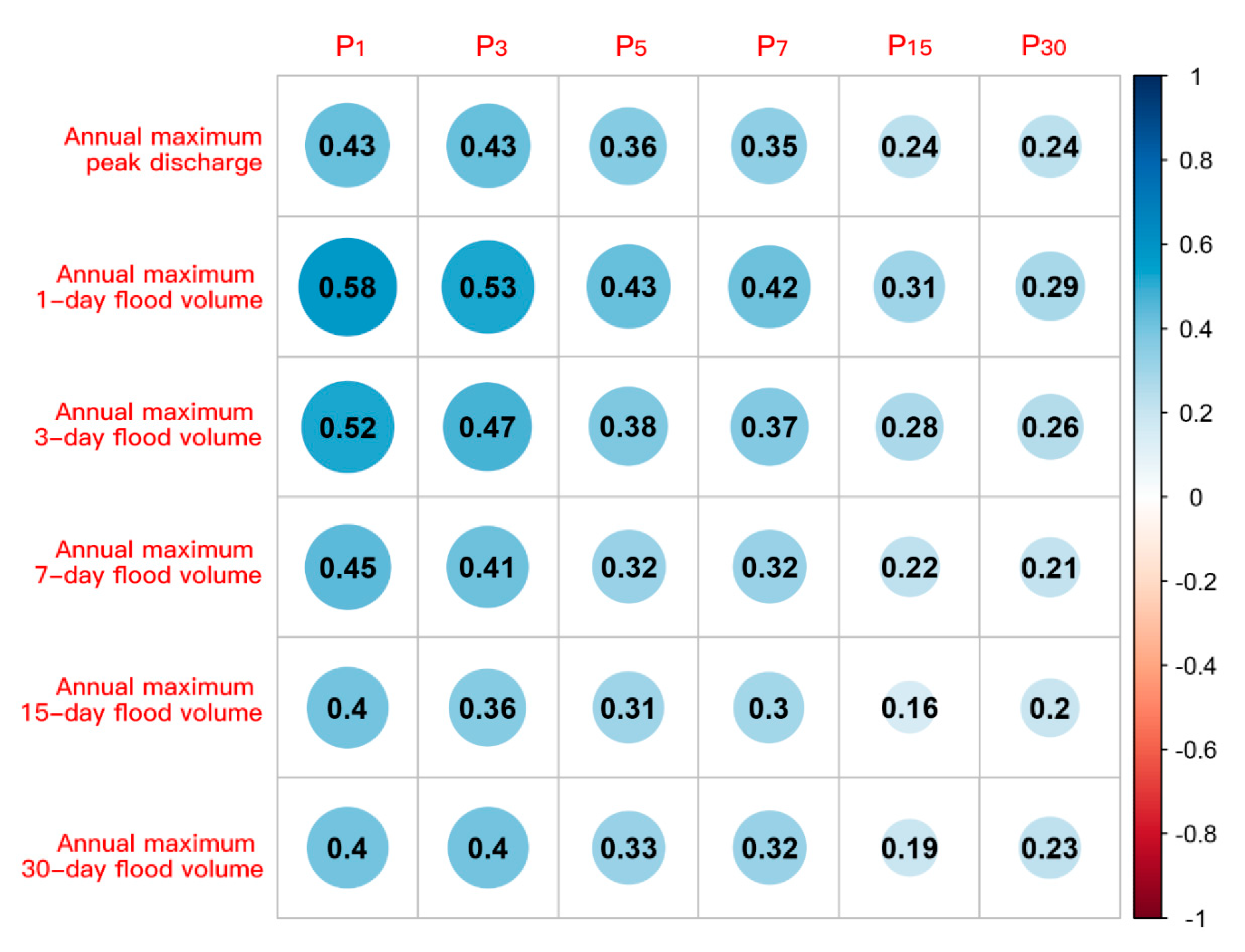
4.2. Correlation Analysis between Precipitation in Early Stage and Snowmelt Flood
4.3. Results with Stationary Approaches: Models 0
4.4. Based on the Results of the Non-Stationary Model with Time Variables: Model 1
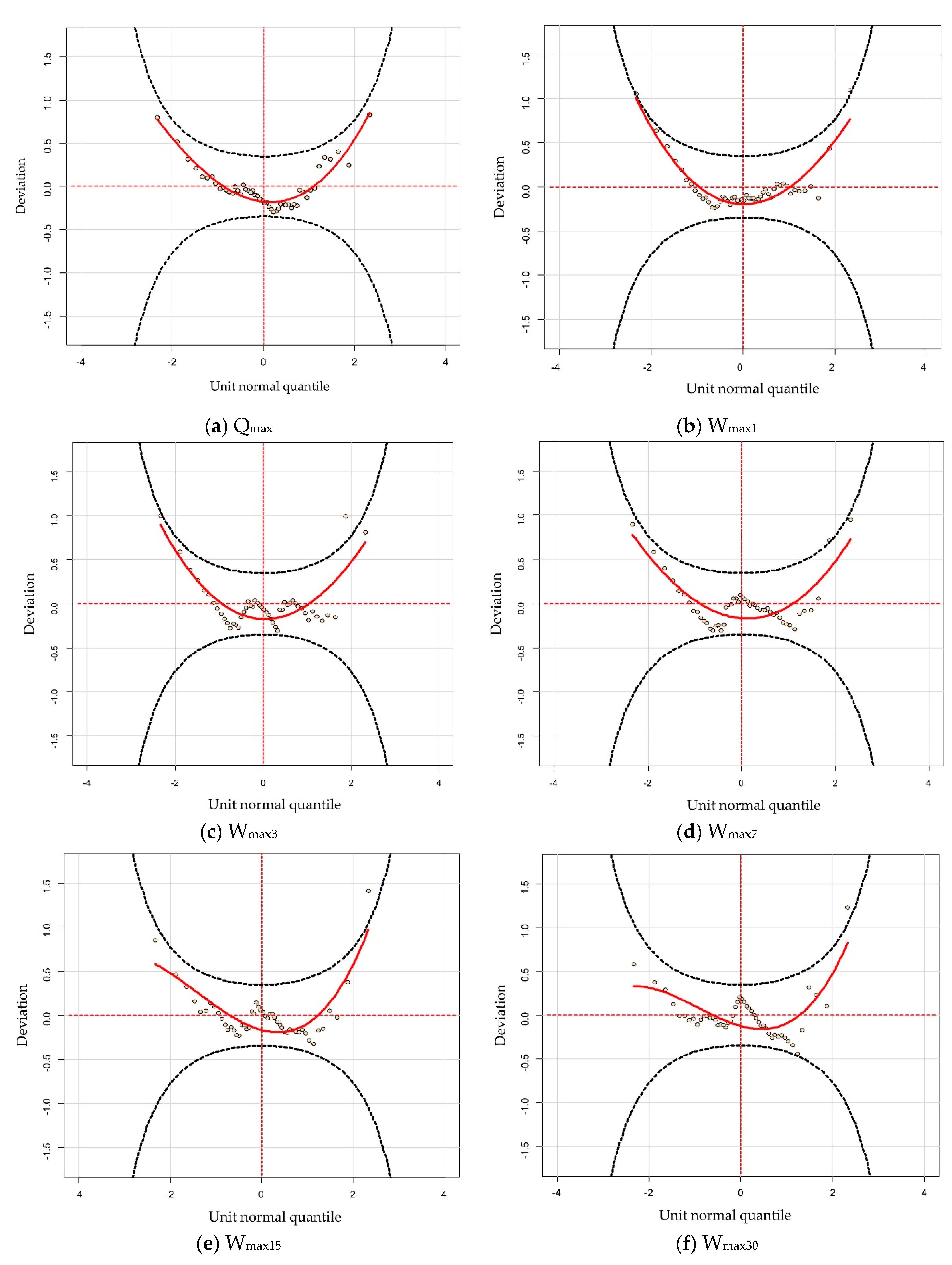
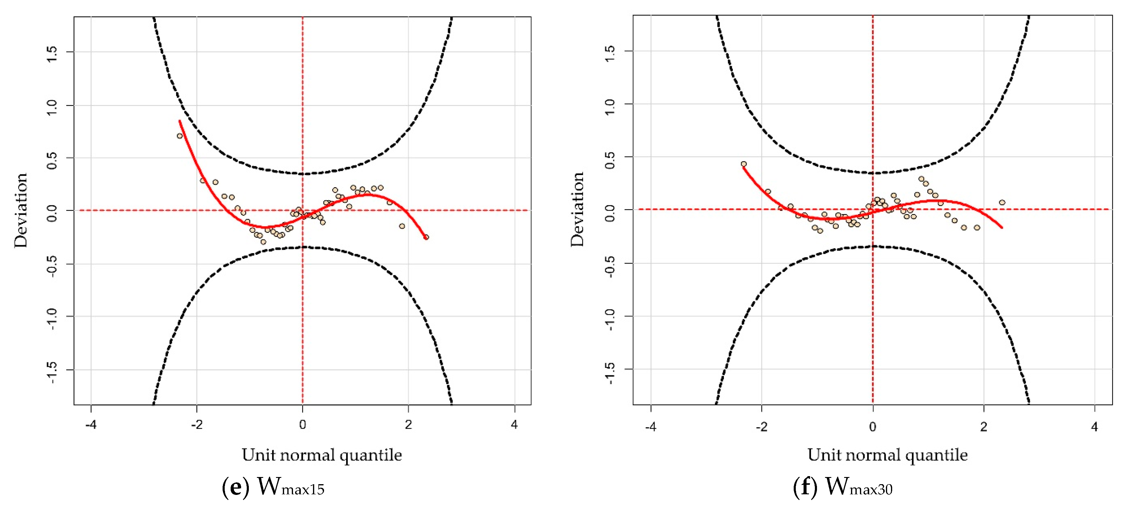
4.4.1. Model Fitting Evaluation
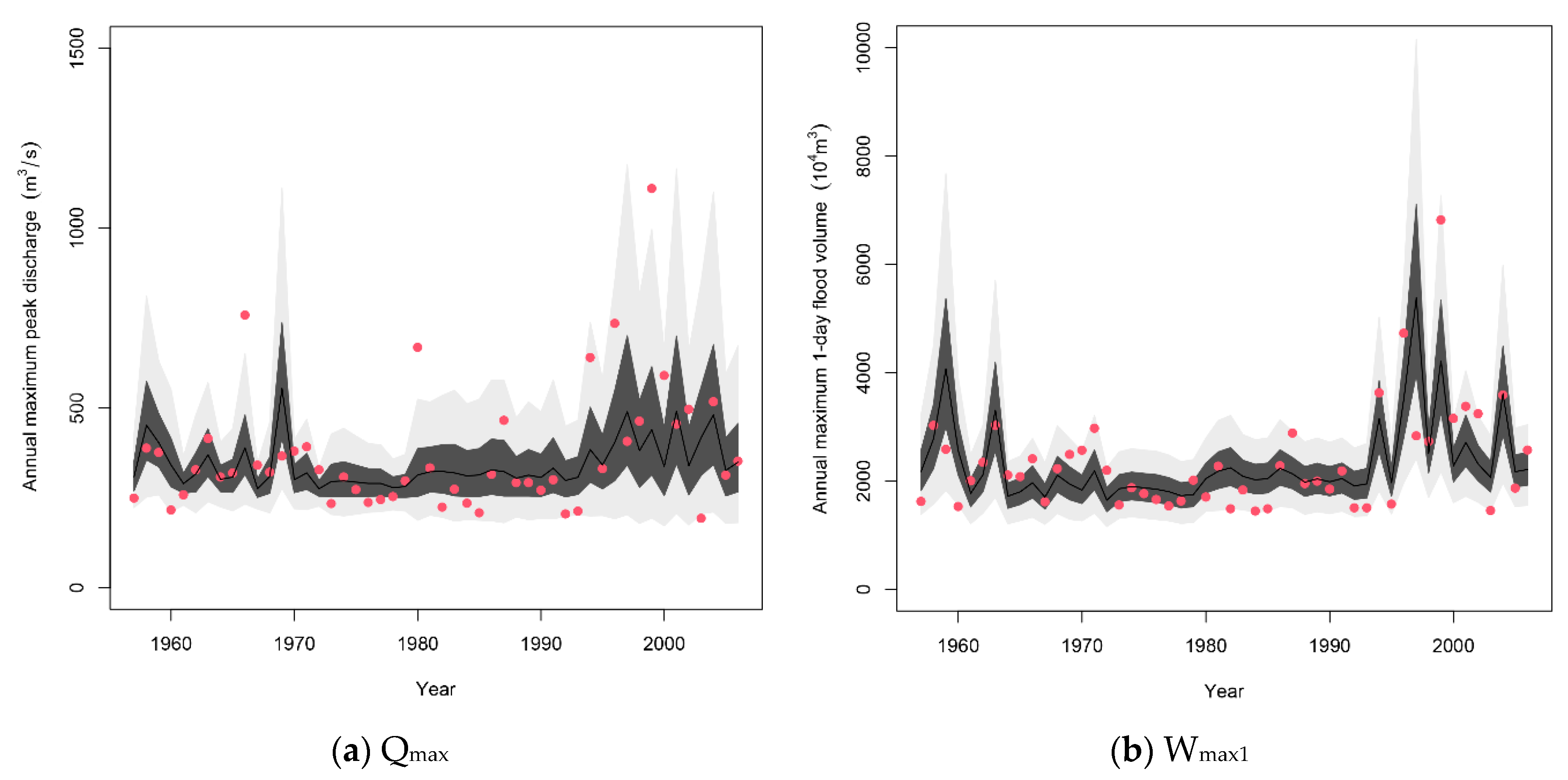
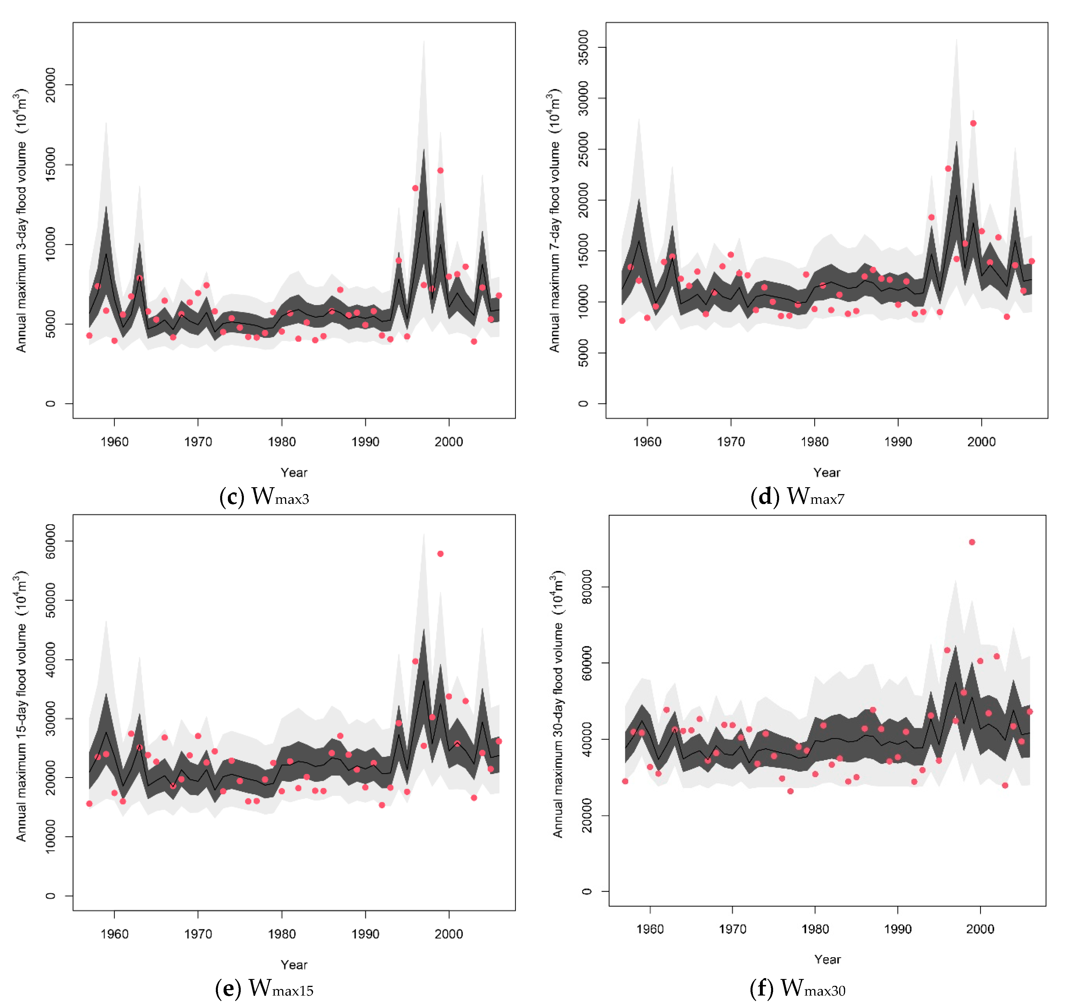
4.4.2. Analysis of Optimal Model Fitting Results
4.5. Based on the Results of the Non-Stationary Model with Climatic Factors: Model 2
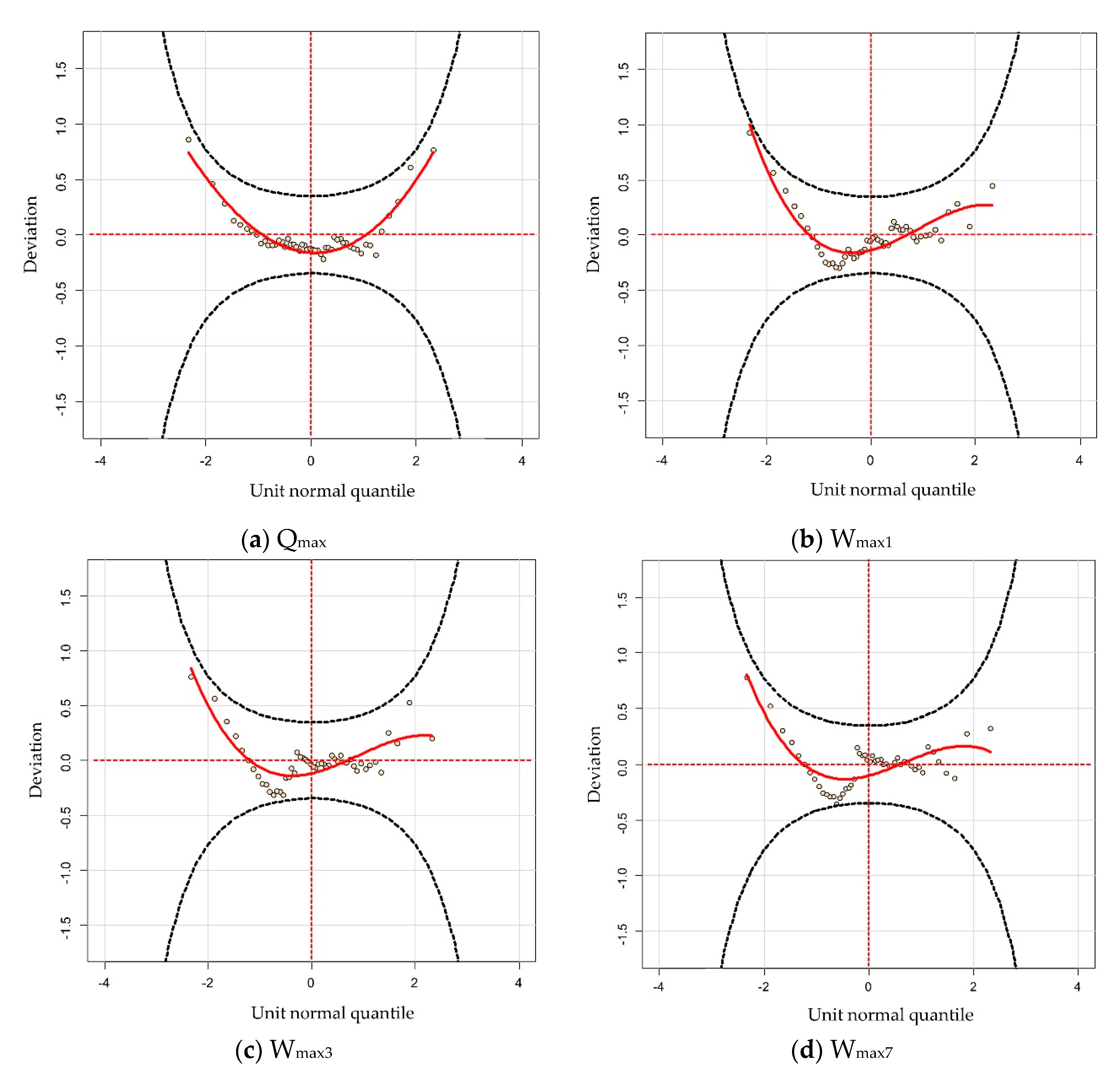
4.5.1. Model Fitting Evaluation
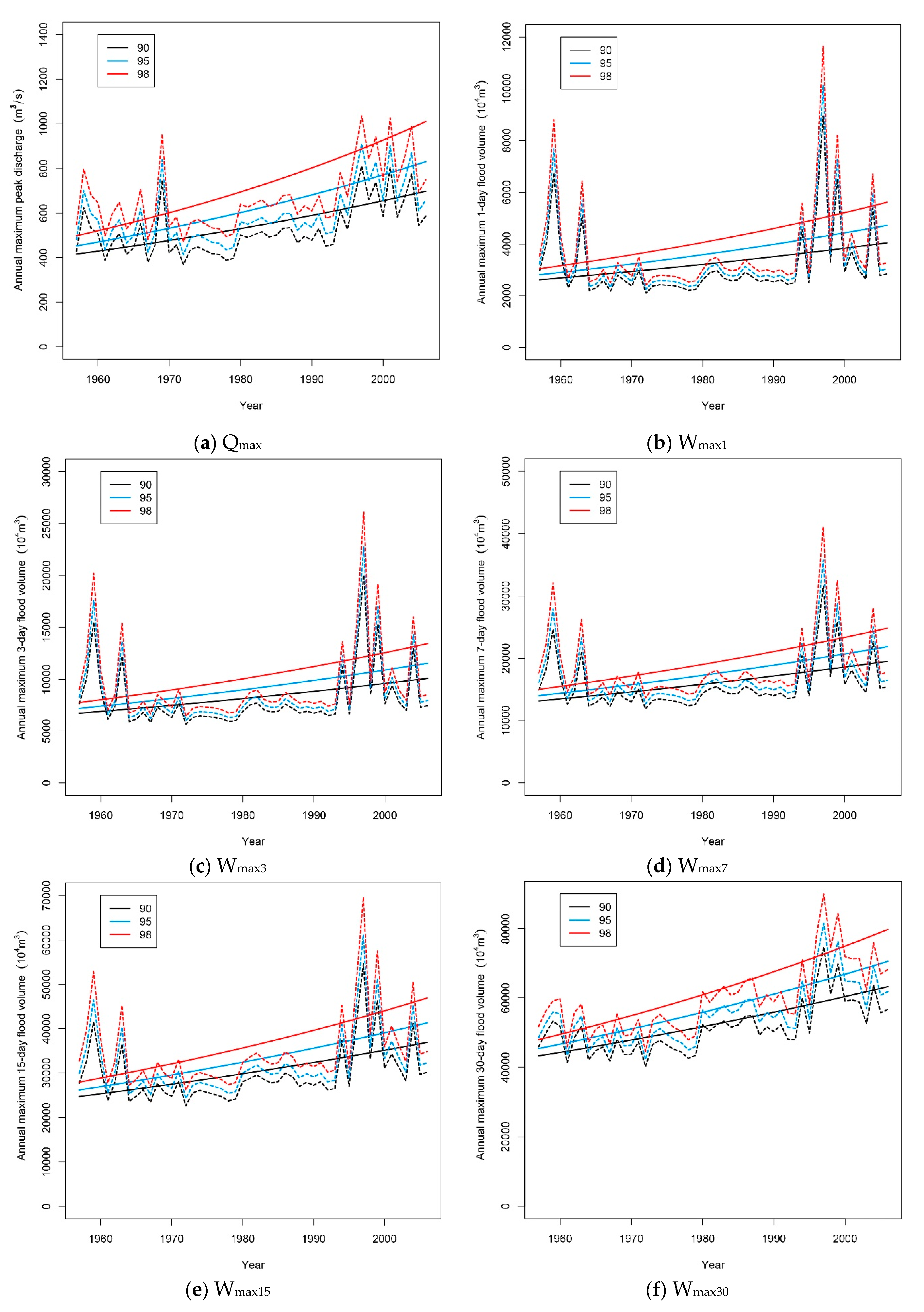
4.5.2. Analysis of Optimal Model Fitting Results
5. Conclusions
Author Contributions
Funding
Institutional Review Board Statement
Informed Consent Statement
Data Availability Statement
Conflicts of Interest
References
- Zveryaev, I.I. Decade-To-Century-Scale Climate Variability and Change: A Science Strategy; National Academy Press: Washington, DC, USA, 2000. [Google Scholar]
- Schmocker-Fackel, P.; Naef, F. More frequent flooding? Changes in flood frequency in Switzerland since 1850. J. Hydrol. 2010, 381, 1–8. [Google Scholar] [CrossRef]
- Todorovic, P.; Rousselle, J. Some Problems of Flood Analysis. Water Resour. Res. 1971, 7, 1144–1150. [Google Scholar] [CrossRef]
- Douglas, E.M.; Vogel, R.M.; Kroll, C.N. Trends in floods and low flows in the United States: Impact of spatial correlation. J. Hydrol. 2000, 240, 90–105. [Google Scholar] [CrossRef]
- Hejazi, M.I.; Markus, M. Impacts of Urbanization and Climate Variability on Floods in Northeastern Illinois. J. Hydrol. Eng. 2009, 14, 606–616. [Google Scholar] [CrossRef] [Green Version]
- Milly, P.C.D.; Dunne, K.A.; Vecchia, A.V. Global pattern of trends in streamflow and water availability in a changing climate. Nature 2005, 438, 347–350. [Google Scholar] [CrossRef] [PubMed]
- Villarini, G.; Smith, J.A.; Serinaldi, F.; Bales, J.; Bates, P.D.; Krajewski, W.F. Flood frequency analysis for nonstationary annual peak records in an urban drainage basin. Adv. Water Resour. 2009, 32, 1255–1266. [Google Scholar] [CrossRef]
- Vogel, R.M.; Yaindl, C.; Walter, M. Nonstationarity: Flood Magnification and Recurrence Reduction Factors in the United States. J. Am. Water Resour. Assoc. 2011, 47, 464–474. [Google Scholar] [CrossRef]
- Wilson, D.; Hisdal, H.; Lawrence, D. Has streamflow changed in the Nordic countries? –Recent trends and comparisons to hydrological projections. J. Hydrol. 2010, 394, 334–346. [Google Scholar] [CrossRef]
- Chen, F.L.; Li, S.F.; Feng, P.; He, X.L.; Long, A.H. Recheck analysis of reservoir extreme flood control risk considering snowmelt flood sequences with jump up components. Adv. Sci. Technol. Water Resour. 2019, 39, 9–16. [Google Scholar]
- He, C.F.; Chen, F.L.; Zhang, Z.Z.; Yang, K.; He, X.L.; Long, A.H. Analysis of variation characteristics of snowmelt flood sequence in the upper Manas River Basin. J. Water Resour. Water Eng. 2020, 31, 109–114. [Google Scholar]
- Chen, F.L.; Wang, Y.X.; Wu, Z.B.; Feng, P. Impacts of Climate Change and Human Activities on Runoff of Continental River in Arid Areas—Taking Kensiwate Hydrological Station in Xinjiang Manas River Basin as an Example. Arid Zone Res. 2015, 32, 692–697. [Google Scholar]
- Ling, H.; Xu, H.; Shi, W.; Zhang, Q. Regional climate change and its effects on the runoff of Manas River, Xinjiang, China. Environ. Earth Sci. 2011, 64, 2203–2213. [Google Scholar] [CrossRef]
- Chen, F.L.; Zhang, X.H.; Feng, P.; He, X.L.; Long, A.H. Fuzzy risk analysis of dam overtopping under inconsistent snowmelt floods. J. Hydroelectr. Eng. 2018, 37, 22–32. [Google Scholar]
- Li, J.; Zheng, Y.; Wang, Y.; Zhang, T.; Feng, P.; Engel, B. Improved Mixed Distribution Model Considering Historical Extraordinary Floods under Changing Environment. Water 2018, 10, 1016. [Google Scholar] [CrossRef] [Green Version]
- Singh, K.P.; Sinclair, R.A. Two-distribution method for flood frequency analysis. J. Hydraul. Div. 1972, 98, 28–44. [Google Scholar]
- Singh, V.P.; Wang, S.X.; Zhang, L. Frequency analysis of nonidentically distributed hydrologic flood data. J. Hydrol. 2005, 307, 175–195. [Google Scholar] [CrossRef]
- Strupczewski, W.G.; Kaczmarek, Z. Non-stationary approach to at-site flood frequency modelling II. Weighted least squares estimation. J. Hydrol. 2001, 248, 143–151. [Google Scholar] [CrossRef]
- Strupczewski, W.G.; Singh, V.P.; Mitosek, H.T. Non-stationary approach to at-site flood frequency modelling. III. Flood analysis of Polish rivers. J. Hydrol. 2001, 248, 152–167. [Google Scholar] [CrossRef]
- Rigby, R.A.; Stasinopoulos, D.M. Generalized additive models for location, scale and shape (with discussion). J. R. Stat. Soc. Ser. C 2005, 54, 507–554. [Google Scholar] [CrossRef] [Green Version]
- Aissaoui-Fqayeh, I.; El-Adlouni, S.; Ouarda, T.B.M.J.; St-Hilaire, A. Développement du modèle log-normal non-stationnaire et comparaison avec le modèle GEV non-stationnaire. Hydrol. Sci. J. 2009, 54, 1141–1156. [Google Scholar] [CrossRef]
- Katz, R.W.; Parlange, M.B.; Naveau, P. Statistics of extremes in hydrology. Adv. Water Resour. 2002, 25, 1287–1304. [Google Scholar] [CrossRef] [Green Version]
- Kwon, H.H.; Brown, C.; Lall, U. Climate informed flood frequency analysis and prediction in Montana using hierarchical Bayesian modeling. Geophys. Res. Lett. 2008, 35, 1–6. [Google Scholar] [CrossRef] [Green Version]
- Ouarda, T.B.M.J.; El-Adlouni, S. Bayesian Nonstationary Frequency Analysis of hydrological variables. J. Am. Water Resour. 2011, 47, 496–505. [Google Scholar] [CrossRef]
- Zhang, F.H.; Hanjra, M.A.; Hua, F.; Shu, Y.Q.; Li, Y.Y. Analysis of climate variability in the Manas River Valley, North-Western China (1956–2006). Mitig. Adapt. Strateg. Glob. Chang. 2014, 19, 1091–1107. [Google Scholar] [CrossRef]
- Ling, H.; Xu, H.; Zhang, Q.; Shi, W. Nonlinear Characteristics of Runoff Processes of the Manas River in Xingjiang. J. Nat. Resour. 2011, 26, 683–693. [Google Scholar]
- Ren, L.; Xue, L.; Liu, Y.; Shi, J.; Han, Q.; Peng, F. Study on Variations in Climatic Variables and Their Influence on Runoff in the Manas River Basin, China. Water 2017, 9, 258. [Google Scholar] [CrossRef] [Green Version]
- Wen, C.; Meng, H.; Ju, L.; Liu, B.; JI, L. Role and impact of Kensiwate hydraulic project in Xinjiang. J. Water Resour. Water Eng. 2015, 26, 156–161. [Google Scholar]
- Jiang, B.; Wang, J. Design and scheme optimization of Kenswat water control project. Water Conserv. Sci. Technol. Econ. 2013, 19, 21–22. [Google Scholar]
- Dutilleul, P.; Stockwell, J.D.; Frigon, D.; Legendre, P. The Mantel test versus Pearson’s correlation analysis: Assessment of the differences for biological and environmental studies. J. Agric. Biol. Environ. Stat. 2000, 5, 131–150. [Google Scholar] [CrossRef]
- Rock, N.M.S. CORANK: A FORTRAN-77 program to calculate and test matrices of Pearson, Spearman, and Kendall correlation coefficients with pairwise treatment of missing values. Comput. Geosci. 1987, 13, 659–662. [Google Scholar] [CrossRef]
- Shih, J.H.; Fay, M.P. Pearson’s chi-square test and rank correlation inferences for clustered data. Biometrics 2017, 73, 822–834. [Google Scholar] [CrossRef] [PubMed]
- Stasinopoulos, D.M.; Rigby, R.A. Generalized additive models for location scale and shape (GAMLSS) in R. J. Stat. Softw. 2007, 23, 1–46. [Google Scholar] [CrossRef] [Green Version]
- Hipel, K. Geophysical model discrimination using the Akaike information criterion. IEEE Trans. Autom. Control 1981, 26, 358–378. [Google Scholar] [CrossRef]
- Filliben, J.J. The Probability Plot Correlation Coefficient Test for Normality. Technometrics 1975, 17, 111. [Google Scholar] [CrossRef]
- Buuren, S.V.; Fredriks, M. Worm plot: A simple diagnostic device for modelling growth reference curves. Stat. Med. 2001, 20, 1259–1277. [Google Scholar] [CrossRef] [PubMed]
- Vinnikov, K.Y. Trends in moments of climatic indices. Geophys. Res. Lett. 2002, 29, 1027. [Google Scholar] [CrossRef] [Green Version]


| Distribution | Probability Density Function | Distribution Moments |
|---|---|---|
| LOGNO | ||
| GA | ||
| GU | ||
| PIG |
| Qmax | Wmax1 | Wmax3 | Wmax7 | Wmax15 | Wmax30 | |
|---|---|---|---|---|---|---|
| r | 0.3673 | 0.3670 | 0.3818 | 0.4030 | 0.4186 | 0.4290 |
| p-value | 0.0087 | 0.0088 | 0.0062 | 0.0037 | 0.0025 | 0.0019 |
| Distribution | Qmax | Wmax1 | Wmax3 | Wmax7 | Wmax15 | Wmax30 |
|---|---|---|---|---|---|---|
| LOGNO | 630.94 | 804.73 | 890.34 | 948.26 | 1010.42 | 1060.20 |
| GA | 638.12 | 811.39 | 895.91 | 952.86 | 1016.10 | 1064.42 |
| GU | 696.45 | 872.56 | 948.20 | 1001.48 | 1075.57 | 1115.66 |
| PIG | 633.01 | 1183.23 | 1307.98 | 1387.78 | 1534.77 | 1582.77 |
| Snowmelt Flood Characteristic Series | Distribution | Mean | Variance | Skewness | Kurtosis | Filliben Coefficient |
|---|---|---|---|---|---|---|
| Qmax | LOGNO | 0 | 1.020 | 0.919 | 3.596 | 0.968 |
| Wmax1 | LOGNO | 0 | 1.020 | 0.958 | 3.976 | 0.961 |
| Wmax3 | LOGNO | 0 | 1.020 | 0.909 | 3.918 | 0.959 |
| Wmax7 | LOGNO | 0 | 1.020 | 0.864 | 3.927 | 0.962 |
| Wmax15 | LOGNO | 0 | 1.020 | 1.072 | 5.089 | 0.959 |
| Wmax30 | LOGNO | 0 | 1.020 | 0.851 | 4.510 | 0.966 |
| Distribution | θ1 | θ2 | GD | AIC | SBC | θ1 | θ2 | GD | AIC | SBC |
| Qmax | Wmax1 | |||||||||
| LOGNO | t | t | 620.22 | 628.22 | 635.86 | t | t | 791.88 | 799.88 | 807.53 |
| GA | t | t | 626.19 | 634.19 | 641.84 | t | t | 795.94 | 803.94 | 811.59 |
| GU | t | t | 677.45 | 685.45 | 693.10 | t | ct | 856.48 | 862.48 | 868.21 |
| PIG | t | ct | 626.37 | 632.37 | 638.10 | t | ct | 1175.83 | 1181.83 | 1187.57 |
| Wmax3 | Wmax7 | |||||||||
| LOGNO | t | t | 878.16 | 886.16 | 893.81 | t | t | 935.70 | 943.70 | 951.35 |
| GA | t | t | 881.42 | 889.42 | 897.07 | t | t | 938.05 | 946.05 | 953.70 |
| GU | t | ct | 931.93 | 937.93 | 943.67 | t | ct | 983.88 | 989.88 | 995.62 |
| PIG | t | ct | 1300.30 | 1306.30 | 1312.04 | t | ct | 1378.81 | 1384.81 | 1390.54 |
| Wmax15 | Wmax30 | |||||||||
| LOGNO | t | t | 996.86 | 1004.86 | 1012.51 | t | t | 1045.25 | 1053.25 | 1060.90 |
| GA | t | t | 999.76 | 1007.76 | 1015.41 | t | t | 1046.86 | 1054.86 | 1062.51 |
| GU | t | ct | 1058.44 | 1064.44 | 1070.18 | t | ct | 1097.66 | 1103.66 | 1109.39 |
| PIG | t | ct | 1525.68 | 1531.68 | 1537.42 | t | ct | 1574.07 | 1580.07 | 1585.81 |
| Snowmelt Flood Characteristic Series | Distribution | Mean | Variance | Skewness | Kurtosis | Filliben Coefficient |
|---|---|---|---|---|---|---|
| Qmax | LOGNO | 0 | 1.020 | 0.830 | 3.562 | 0.977 |
| Wmax1 | LOGNO | 0 | 1.020 | 0.543 | 2.563 | 0.977 |
| Wmax3 | LOGNO | 0 | 1.020 | 0.476 | 2.577 | 0.978 |
| Wmax7 | LOGNO | 0 | 1.020 | 0.379 | 2.420 | 0.979 |
| Wmax15 | LOGNO | 0 | 1.020 | 0.457 | 2.921 | 0.982 |
| Wmax30 | LOGNO | 0 | 1.020 | 0.180 | 2.665 | 0.990 |
| Distribution | θ1 | θ2 | GD | AIC | SBC | θ1 | θ2 | GD | AIC | SBC |
| Qmax | Wmax1 | |||||||||
| LOGNO | T78 + P3 | t | 610.08 | 618.08 | 625.73 | T78 + P1 | P1 | 765.05 | 775.05 | 784.61 |
| GA | T78 + P3 | ct | 612.61 | 620.61 | 628.26 | T78 + P1 | P1 | 764.72 | 774.72 | 784.28 |
| GU | T78 + P3 | ct | 661.83 | 669.83 | 677.48 | T78 + P1 | P1 | 779.19 | 789.19 | 798.75 |
| PIG | P3 | ct | 621.21 | 627.21 | 632.94 | T78 | P1 | 1164.72 | 1172.72 | 1180.37 |
| Wmax3 | Wmax7 | |||||||||
| LOGNO | T78 + P1 | P1 | 856.04 | 866.04 | 875.60 | T78 + P1 | P1 | 919.13 | 929.13 | 938.69 |
| GA | T78 + P1 | P1 | 855.85 | 865.85 | 875.41 | T78 + P1 | P1 | 919.56 | 929.56 | 939.12 |
| GU | T78 + P1 | T78 + P1 | 865.91 | 877.91 | 889.38 | T78 + P1 | P1 | 933.82 | 943.82 | 953.38 |
| PIG | T78 + P1 | ct | 1278.51 | 1286.51 | 1294.15 | P1 | ct | 1371.10 | 1377.10 | 1382.84 |
| Wmax15 | Wmax30 | |||||||||
| LOGNO | T78 + P1 | P1 | 983.80 | 993.80 | 1003.36 | T78 + P1 | T78 | 1035.10 | 1045.10 | 1054.66 |
| GA | T78 + P1 | P1 | 984.95 | 994.95 | 1004.51 | T78 + P1 | T78 | 1035.91 | 1045.91 | 1055.47 |
| GU | T78 + P1 | P1 | 1005.48 | 1015.48 | 1025.04 | T78 + P1 | P1 | 1056.75 | 1066.75 | 1076.31 |
| PIG | T78 | ct | 1521.19 | 1527.19 | 1532.99 | ct | ct | 1578.77 | 1582.77 | 1586.60 |
| Snowmelt Flood Characteristic Series | Distribution | Mean | Variance | Skewness | Kurtosis | Filliben Coefficient |
|---|---|---|---|---|---|---|
| Qmax | LOGNO | 0 | 1.020 | 0.352 | 3.425 | 0.985 |
| Wmax1 | GA | 0 | 1.011 | 0.007 | 1.896 | 0.986 |
| Wmax3 | GA | 0 | 1.019 | 0.015 | 1.863 | 0.987 |
| Wmax7 | LOGNO | 0 | 1.020 | 0.082 | 1.795 | 0.985 |
| Wmax15 | LOGNO | 0 | 1.020 | 0.246 | 1.916 | 0.983 |
| Wmax30 | LOGNO | 0 | 1.020 | 0.108 | 2.194 | 0.992 |
| Snowmelt Flood Characteristic Series | Extremum | Year | Quantile of Snowmelt Flood Time Series | Design Standard Value | ||||
|---|---|---|---|---|---|---|---|---|
| 98% | 95% | 90% | 50-Year | 20-Year | 10-Year | |||
| Annual maximum peak discharge (m3/s) | maximum | 1996 | 1459 | 1172 | 966 | 1249 | 856 | 600 |
| minimum | 1972 | 351 | 341 | 328 | ||||
| Annual maximum 1-day flood volume (105 m3) | maximum | 1996 | 11,636 | 10,141 | 8937 | 7406 | 5206 | 3756 |
| minimum | 1972 | 2013 | 2215 | 2077 | ||||
| Annual maximum 3-day flood volume (105 m3) | maximum | 1996 | 26,029 | 22,623 | 19,998 | 15,920 | 12,090 | 9425 |
| minimum | 1972 | 6424 | 5984 | 5578 | ||||
| Annual maximum 7-day flood volume (105 m3) | maximum | 1996 | 41,058 | 35,625 | 31,400 | 29,430 | 23,120 | 18,620 |
| minimum | 1972 | 13,721 | 12,744 | 11,939 | ||||
| Annual maximum15-day flood volume (105 m3) | maximum | 1996 | 69,712 | 61,205 | 54,513 | 56,830 | 44,230 | 35,340 |
| minimum | 1972 | 26,262 | 24,281 | 22,759 | ||||
| Annual maximum 30-day flood volume (105 m3) | maximum | 1996 | 89,702 | 80,799 | 74,637 | 93,383 | 74,599 | 61,042 |
| minimum | 1972 | 44,883 | 42,446 | 40,431 | ||||
Publisher’s Note: MDPI stays neutral with regard to jurisdictional claims in published maps and institutional affiliations. |
© 2021 by the authors. Licensee MDPI, Basel, Switzerland. This article is an open access article distributed under the terms and conditions of the Creative Commons Attribution (CC BY) license (https://creativecommons.org/licenses/by/4.0/).
Share and Cite
He, C.; Chen, F.; Long, A.; Luo, C.; Qiao, C. Frequency Analysis of Snowmelt Flood Based on GAMLSS Model in Manas River Basin, China. Water 2021, 13, 2007. https://doi.org/10.3390/w13152007
He C, Chen F, Long A, Luo C, Qiao C. Frequency Analysis of Snowmelt Flood Based on GAMLSS Model in Manas River Basin, China. Water. 2021; 13(15):2007. https://doi.org/10.3390/w13152007
Chicago/Turabian StyleHe, Chaofei, Fulong Chen, Aihua Long, Chengyan Luo, and Changlu Qiao. 2021. "Frequency Analysis of Snowmelt Flood Based on GAMLSS Model in Manas River Basin, China" Water 13, no. 15: 2007. https://doi.org/10.3390/w13152007
APA StyleHe, C., Chen, F., Long, A., Luo, C., & Qiao, C. (2021). Frequency Analysis of Snowmelt Flood Based on GAMLSS Model in Manas River Basin, China. Water, 13(15), 2007. https://doi.org/10.3390/w13152007