
Simulation of Water and Salt Dynamics under Different Water-Saving Degrees Using the SAHYSMOD Model


 and
and
Abstract
:1. Introduction
2. Materials and Methods
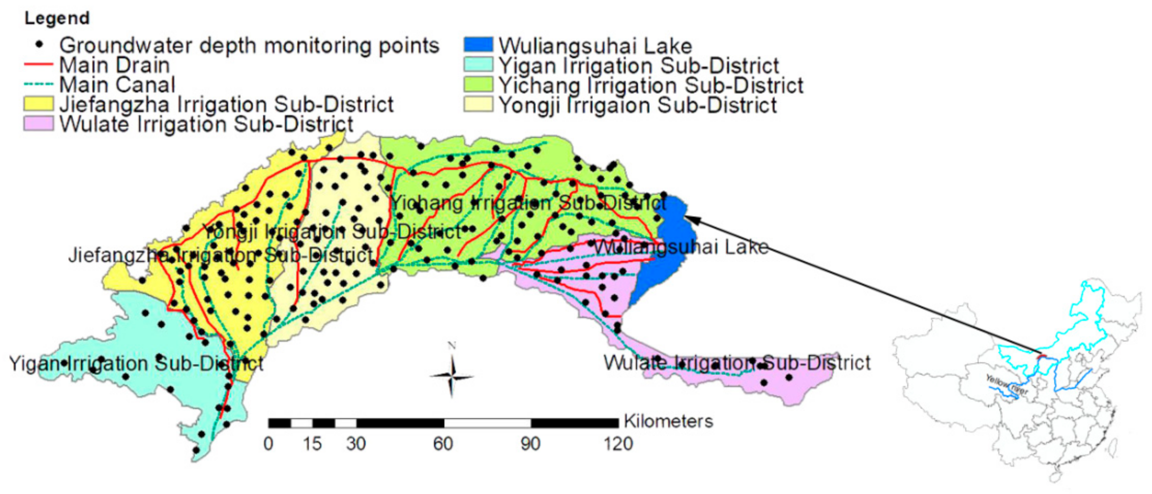
2.1. Study Area
2.2. SAHYSMOD Model Description
2.2.1. Technical Details of SAHYSMOD
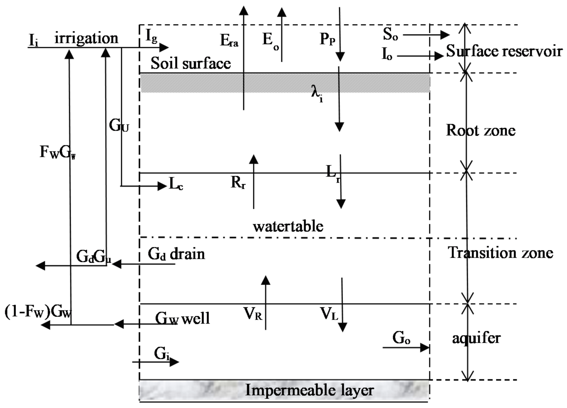
2.2.2. Principles of SAHYSMOD
2.2.3. Data Required
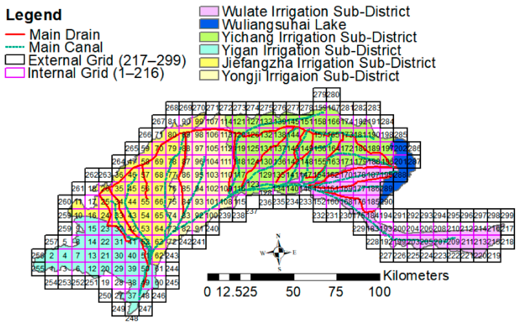
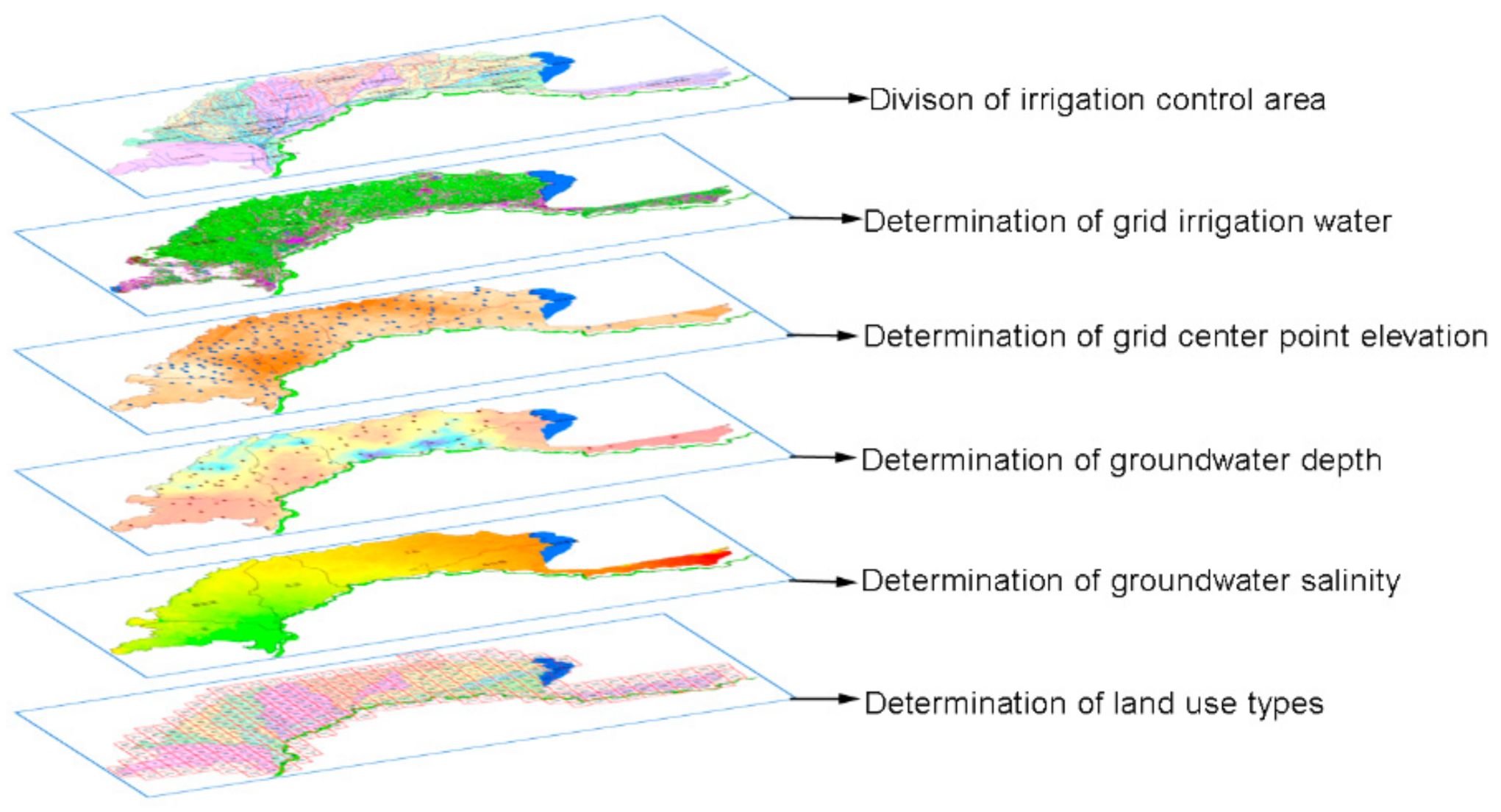
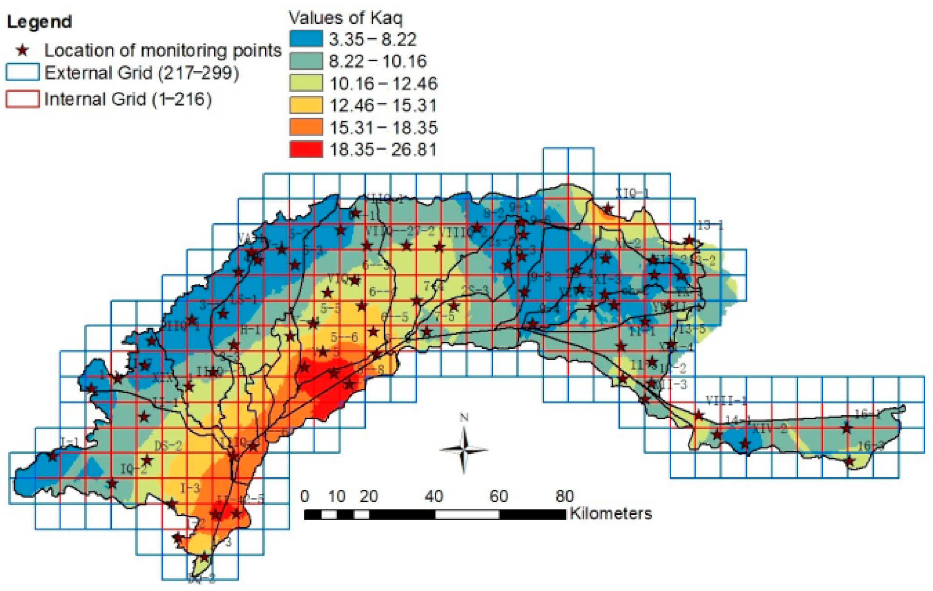
2.2.4. Grid Generation in the Study Area
3. Results and Discussion
3.1. Calibration and Validation of SAHYSMOD
3.1.1. Determining Kaq
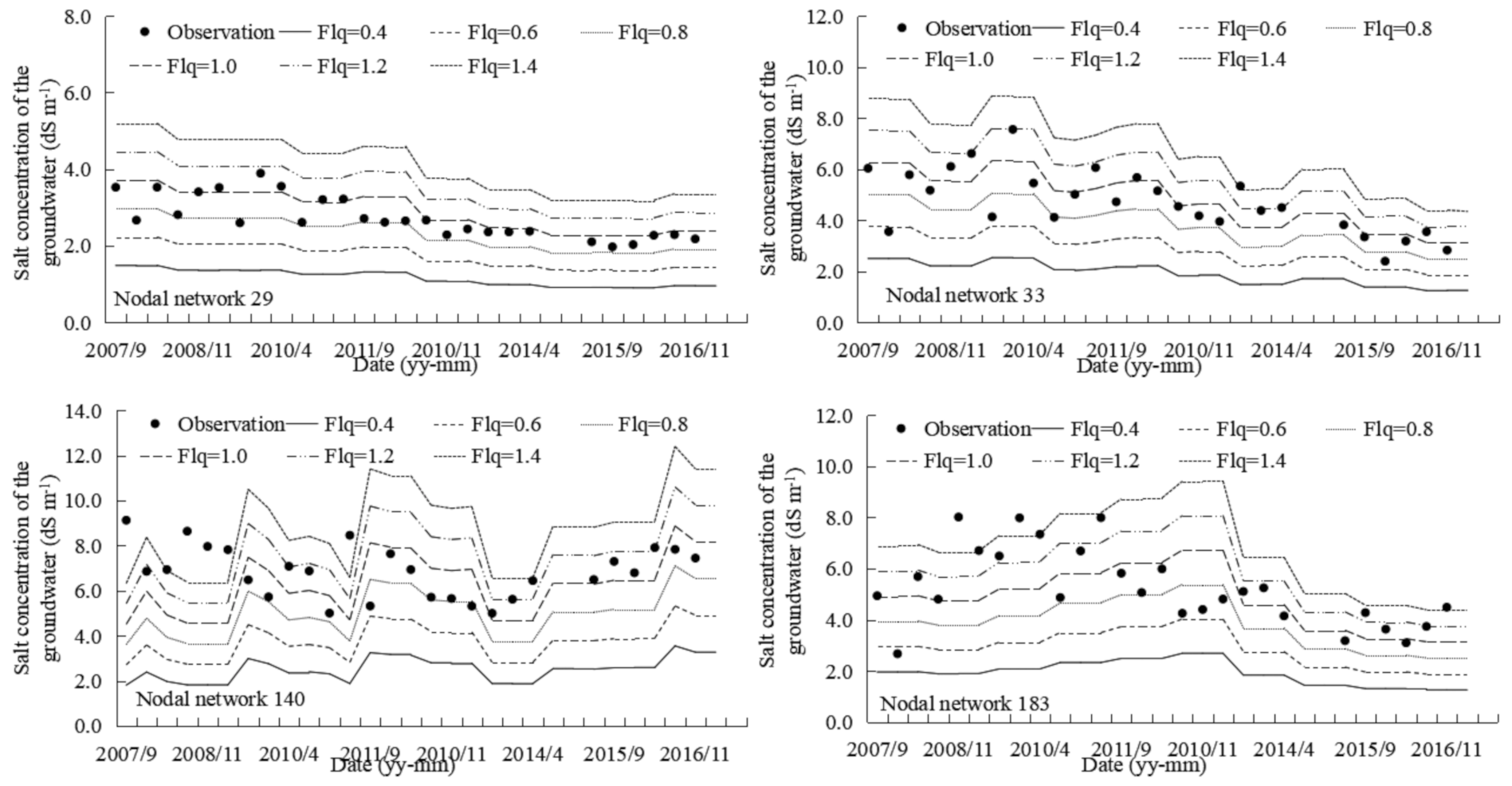
3.1.2. Determining Flq
3.1.3. Error Analysis
3.2. Scenario Setting
3.3. Scenario Simulation
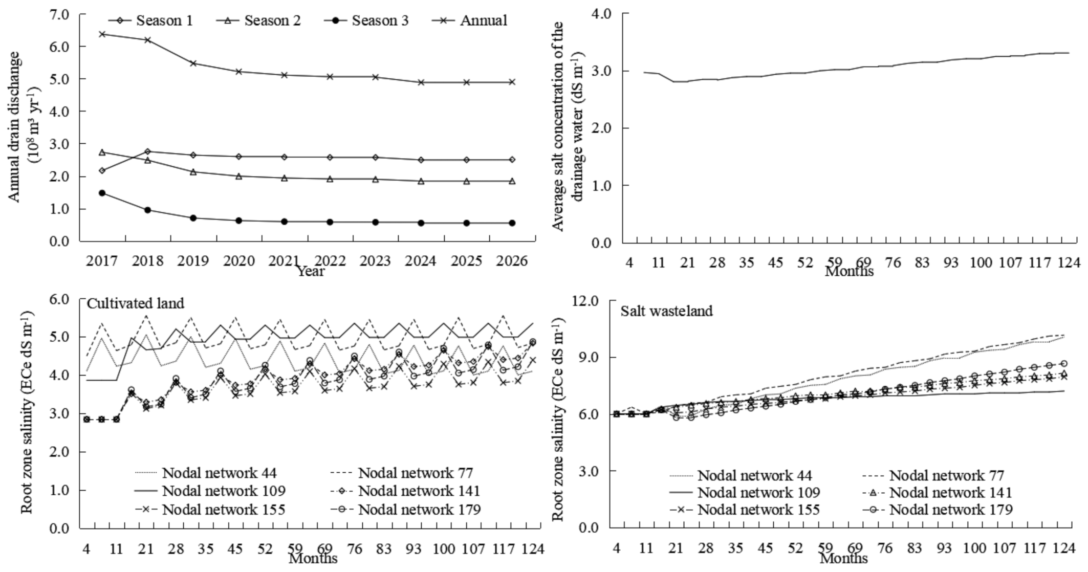
3.3.1. Current Irrigation and Drainage Management Scheme
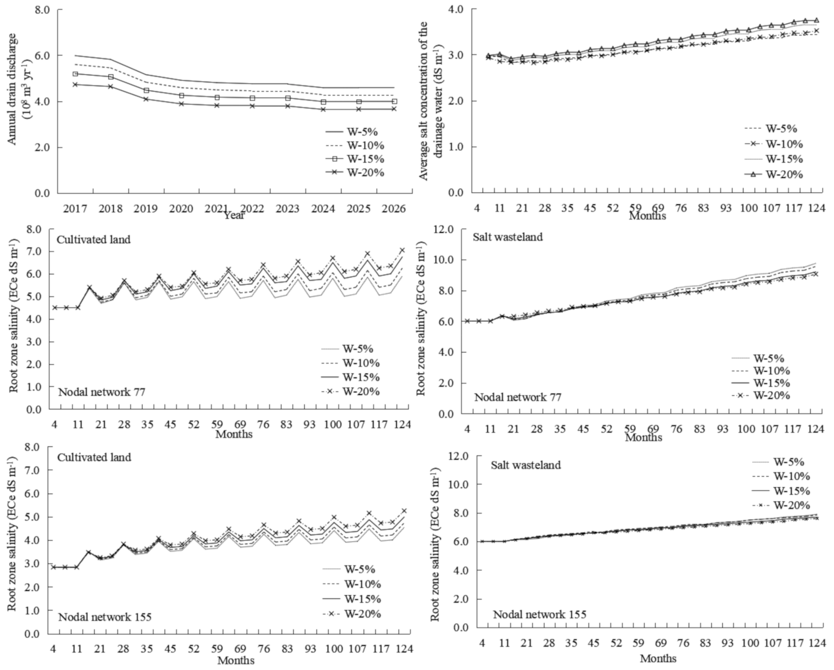
3.3.2. Schemes for Reducing Total Water Diversion from the Canal Head
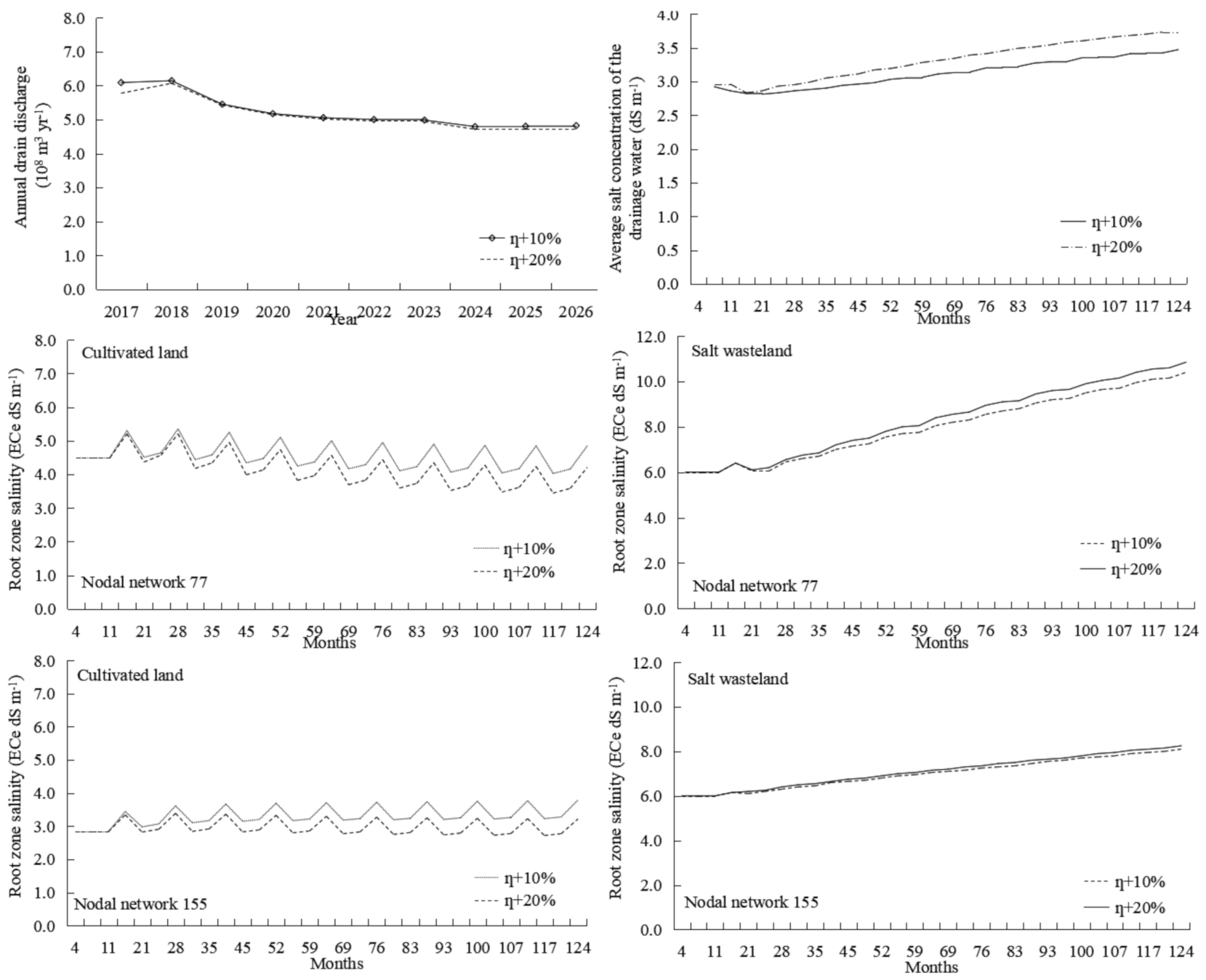
3.3.3. Schemes for Improving the Water Efficiency of the Canal System
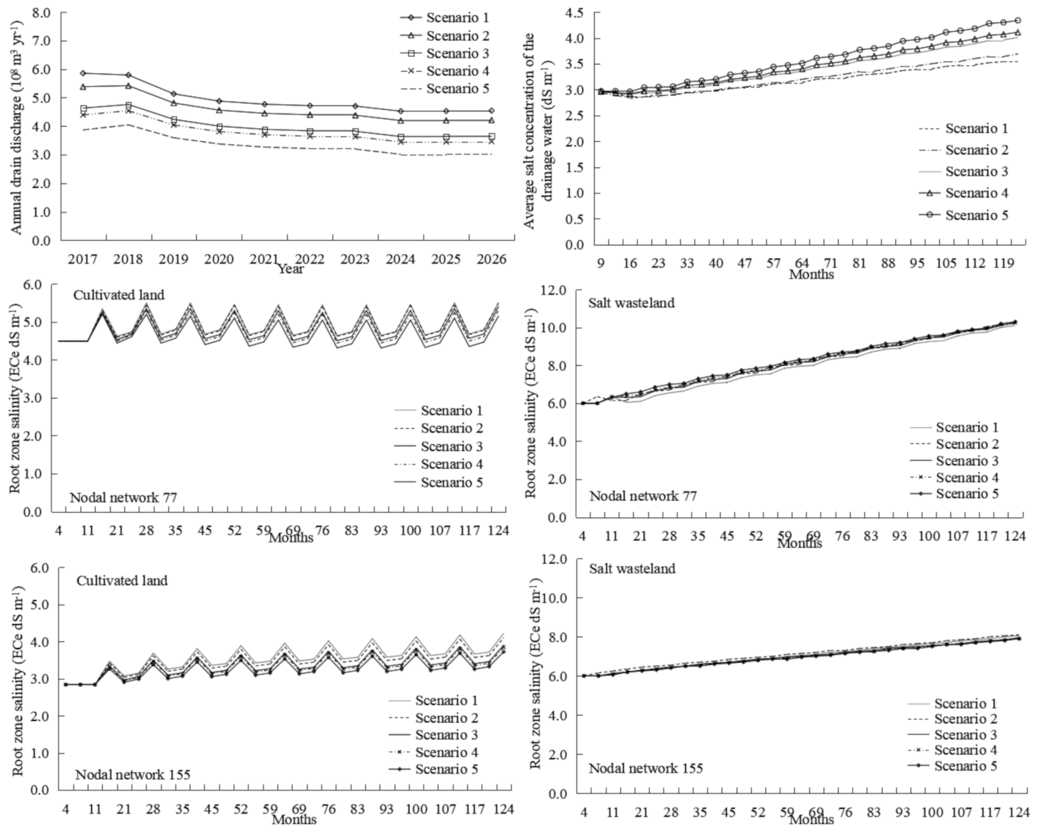
3.3.4. Different Water-Saving Schemes
3.3.5. Comparative Analysis of Different Schemes
4. Conclusions
Author Contributions
Funding
Institutional Review Board Statement
Informed Consent Statement
Data Availability Statement
Conflicts of Interest
References
- Mirlas, V. Assessing soil salinity hazard in cultivated areas using MODFLOW model and GIS tools: A case study from the Jezre’el Valley, Israel. Agric. Water Manag. 2012, 109, 144–154. [Google Scholar] [CrossRef]
- Xu, X.; Huang, G.H.; Qu, Z.Y.; Pereira, L. Assessing the groundwater dynamics and impacts of water saving in the Hetao Irrigation District, Yellow River basin. Agric. Water Manag. 2010, 98, 301–313. [Google Scholar] [CrossRef]
- Yang, Y.T.; Shang, S.H.; Jiang, L. Remote sensing temporal and spatial patterns of evapotranspiration and the responses to water management in a large irrigation district of North China. Agric. For. Meteorol. 2012, 164, 112–122. [Google Scholar] [CrossRef]
- Yue, W.F.; Li, X.Z.; Wang, T.J.; Chen, X.H. Impacts of water saving on groundwater balance in a large-scale arid irrigation district, Northwest China. Irrig. Sci. 2016, 34, 297–312. [Google Scholar] [CrossRef]
- Chen, L.J.; Feng, Q.; Li, F.R.; Li, C.S. Simulation of soil water and salt transfer under mulched furrow irrigation with saline water. Geoderma 2015, 241–242, 87–96. [Google Scholar] [CrossRef]
- Pereira, L.S.; Goncalves, J.M.; Dong, B.; Mao, Z.; Fang, S.X. Assessing basin irrigation and scheduling strategies for saving irrigation water and controlling salinity in the upper Yellow River Basin, China. Agric. Water Manag. 2007, 93, 109–122. [Google Scholar] [CrossRef]
- Miao, Q.F.; Shi, H.B.; Goncalves, J.M.; Pereira, L. Field assessment of basin irrigation performance and water saving in Hetao, Yellow River basin: Issues to support irrigation systems modernisation. Biosyst. Eng. 2015, 136, 102–116. [Google Scholar] [CrossRef] [Green Version]
- Lekakis, E.H.; Antonopoulos, V.Z. Modeling the effects of different irrigation water salinity on soil water movement, uptake and multicomponent solute transport. J. Hydrol. 2015, 530, 431–446. [Google Scholar] [CrossRef]
- Chen, L.J.; Feng, Q.; Li, F.R.; Li, C.S. A bidirectional model for simulating soil water flow and salt transport under mulched drip irrigation with saline water. Agric. Water Manag. 2014, 146, 24–33. [Google Scholar] [CrossRef]
- Qi, Z.J.; Feng, H.; Zhao, Y.; Zhang, T.B.; Yang, A.Z.; Zhang, Z.X. Spatial distribution and simulation of soil moisture and salinity under mulched drip irrigation combined with tillage in an arid saline irrigation district, northwest China. Agric. Water Manag. 2018, 201, 219–231. [Google Scholar] [CrossRef]
- Jiang, J.; Feng, S.Y.; Huo, Z.L.; Zhao, Z.C.; Jia, B. Application of the SWAP model to simulate water–salt transport under deficit irrigation with saline water. Math. Comput. Model 2011, 54, 902–911. [Google Scholar] [CrossRef]
- Yao, R.J.; Yang, J.S.; Zhang, T.J.; Hong, L.Z.; Wang, M.W.; Yu, S.P.; Wang, X.P. Studies on soil water and salt balances and scenarios simulation using SaltMod in a coastal reclaimed farming area of eastern China. Agric. Water Manag. 2014, 131, 115–123. [Google Scholar] [CrossRef]
- Singh and Ajay. Evaluating the effect of different management policies on the long-term sustainability of irrigated agriculture. Land Use Policy 2016, 54, 499–507. [Google Scholar] [CrossRef]
- Mao, W.; Yang, J.S.; Zhu, Y.; Ye, M.; Wu, J.W. Loosely coupled SaltMod for simulating groundwater and salt dynamics under well-canal conjunctive irrigation in semi-arid areas. Agric. Water Manag. 2017, 192, 209–220. [Google Scholar] [CrossRef]
- Chang, X.M.; Gao, Z.Y.; Wang, S.L.; Chen, H.R. Modelling long-term soil salinity dynamics using SaltMod in Hetao Irrigation District, China. Comput. Electron. Agric. 2019, 156, 447–458. [Google Scholar] [CrossRef]
- Fujimaki, H.; Abd, H.M.; Mahdavi, S.M.; Ebrahimian, H. Optimization of Irrigation and Leaching Depths Considering the Cost of Water Using WASH_1D/2D Models. Water 2020, 12, 2549. [Google Scholar] [CrossRef]
- Surendran, U.; Sushanth, C.M.; Mammen, G.; Joseph, E.J. Modelling the Crop Water Requirement Using FAO-CROPWAT and Assessment of Water Resources for Sustainable Water Resource Management: A Case Study in Palakkad District of Humid Tropical Kerala, India. Aquat. Procedia 2015, 4, 1211–1219. [Google Scholar] [CrossRef]
- Xu, X.; Huang, G.H.; Qu, Z.Y.; Pereira, L.S. Using MODFLOW and GIS to Assess Changes in Groundwater Dynamics in Response to Water Saving Measures in Irrigation Districts of the Upper Yellow River Basin. Water Resour. Manag. 2011, 25, 2035–2059. [Google Scholar] [CrossRef]
- Xu, X.; Huang, G.H.; Zhan, H.B.; Qu, Z.Y.; Huang, Q.Z. Integration of SWAP and MODFLOW-2000 for modeling groundwater dynamics in shallow water table areas. J. Hydrol. 2012, 412, 170–181. [Google Scholar] [CrossRef]
- Oosterbaan, R.J. SAHYSMOD (Version 1.7a), Description of Principles, User Manual and Case Studies; International Institute for Land Reclamation and Improvement (ILRI): Wageningen, The Netherlands, 2005. [Google Scholar]
- Akram, S.; Kashkouli, H.A.; Pazira, E. Sensitive variables controlling salinity and water table in a bio-drainage system. Irrig. Drain. Sys. 2008, 22, 271–285. [Google Scholar] [CrossRef]
- Desta, T.F. Spatial Modelling and Timely Prediction of Salinization using SAHYSMOD 972 in GIS Environment (a Case Study of Nakhon Ratchasima, Thailand). Master’s Thesis, International Institute for Geo-information Science and Earth Observation, Enschede, The Netherlands, 2009. [Google Scholar]
- Singh, A.; Panda, S.N. Integrated Salt and Water Balance Modeling for the Management of Waterlogging and Salinization. I: Validation of SAHYSMOD. J. Irrig. Drain. Eng. 2012, 138, 955–963. [Google Scholar] [CrossRef]
- Singh, A.; Panda, S.N. Integrated Salt and Water Balance Modeling for the Management of Waterlogging and Salinization. II: Application of SAHYSMOD. J. Irrig. Drain. Eng. 2012, 138, 964–971. [Google Scholar] [CrossRef]
- Yao, R.J.; Wang, X.J.; Wu, D.H.; Xie, W.P. Calibration and Sensitivity Analysis of Sahysmod for Modeling Field Soil and Groundwater Salinity Dynamics in Coastal Rainfed Farmland. Irrig. Drain. 2017, 66, 411–427. [Google Scholar] [CrossRef]
- Yao, R.L.; Wang, X.J.; Wu, D.H.; Xie, W.P.; Wang, X.P.; Zhang, X. Scenario simulation of field soil water and salt balances using SahysMod for salinity management in a coastal rainfed farmland. Irrig. Drain. 2017, 66, 872–883. [Google Scholar] [CrossRef]
- Inam, A.; Adamowski, J.; Prasher, S.; Halbe, J.; Malard, J.; Albano, R. Coupling of a distributed stakeholder-built system dynamics socio-economic model with SAHYSMOD for sustainable soil salinity management-Part 1: Model development. J. Hydrol. 2017, 551, 278–299. [Google Scholar] [CrossRef]
- Xue, J.; Ren, L. Assessing water productivity in the Hetao Irrigation District in Inner Mongolia by an agro-hydrological model. Irrig. Sci. 2017, 35, 357–382. [Google Scholar] [CrossRef]
- Luo, Y.; Sophocleous, M. Two-way coupling of unsaturated-saturated flow by integrating the SWAT and MODFLOW models with application in an irrigation district in arid region of West China. J. Arid. Land. 2011, 3, 164–173. [Google Scholar] [CrossRef] [Green Version]
- Oosterbaan, R.J. SAHYSMOD, Description of Principles, User Manual and Case Studies; International Institute for Land Reclamation and Improvement: Wageningen, The Netherlands, 1995. [Google Scholar]
- Allen, R.G.; Pereira, L.S.; Raes, D.; Smith, M. Crop Evapotranspiration Guidelines for Computing Crop Water Requirements. FAO Irrigation Drainage Paper 56. 1998. Available online: http://www.avwatermaster.org/filingdocs/195/70653/172618e_5xAGWAx8.pdf. (accessed on 9 July 2021).
- Dai, J.X.; Shi, H.B.; Tian, D.L.; Xai, Y.H.; Hua, L.M. Determined of crops coeffi-cients of mian grain and oil crops in Inner Mongolia Hetao irrigated Area. J. Irrig. Drian. 2011, 30, 23–27. (In Chinese) [Google Scholar]
- Huang, Y.J.; Li, Z.; Zhuo, Z.Q.; Xing, A.; Huang, Y.F. Soil water and salt dynamics under different irrigation and drainage management scenarios based on SahysMod model. Trans. Chin. Soc. Agric. Eng. 2020, 36, 129–140. (In Chinese) [Google Scholar]
- Xu, X.; Huang, G.H.; Sun, C.; Pereira, L.S.; Ramos, T.B.; Huang, Q.Z.; Hao, Y.Y. Assessing the effects of water table depth on water use, soil salinity and wheat yield: Searching for a target depth for irrigated areas in the upper Yellow River basin. Agric. Water Manag. 2013, 125, 46–60. [Google Scholar] [CrossRef]
- Ren, D.Y.; Xu, X.; Hao, Y.Y.; Huang, G.H. Modeling and assessing field irrigation water use in a canal system of Hetao, upper Yellow River basin: Application to maize, sunflower and watermelon. J. Hydrol. 2016, 532, 122–139. [Google Scholar] [CrossRef]


| Seasonal Data | Value | Data Sources |
|---|---|---|
| 1. Duration of seasons (months) | ||
| Season 1 (May–September) | 5 | M |
| Season 2 (October–November) | 2 | M |
| Season 3 (December–April) | 5 | M |
| 2.Water balance components | ||
| Irrigated area fraction in season 1/season 2/season 3 | 0.57/0.57/0 | R |
| Rainfall in season 1/season 2/season 3 (m) | 0.119/0.010/0.011 | M |
| Irrigation in season 1/season 2/season 3 (m) | 0.011–0.506/0.014–0.262/0 | M |
| Seasonal potential evapotranspiration (m) | 0.652–0.694/0.103–0.109/0.062–0.110 | M |
| Salinity of irrigation water season 1/season 2/season 3 (dS m–1) | 1.02 | M |
| Seasonal runoff (m) | 0 | M |
| Rootzone storage efficiency for rainfall and irrigation | 0.8 | M/G |
| Pumped well water from aquifer (m) | 0 | M |
| Polygonal Data | Value | Data Sources |
|---|---|---|
| 1.Overall system parameters | ||
| bottom level of the aquifer | 0 | M |
| Thickness of the surface reservoir (m) | 0 | M |
| Thickness of the root zone (m) | 1 | M |
| Thickness of the transition zone (m) | 4 | M |
| Thickness of the aquifer zone (m) | 90 | M |
| Index for phreatic or semi-confined aquifer (0 = phreatic,1 = semi-confined) | 0 | M |
| 2.Soil and aquifer properties | ||
| Total porosity of the root zone (Ptr) | 0.48 | G |
| Total porosity of the transition zone (Ptx) | 0.48 | G |
| Total porosity of the aquifer zone (Ptq) | 0.4 | G |
| Effective porosity of the root zone (Per) | 0.07 | G |
| Effective porosity of the transition zone (Pex) | 0.07 | G |
| Effective porosity of the aquifer zone (Peq) | 0.1 | G |
| Leaching efficiency of the root zone (Flr) | 0.85 | G/C |
| Leaching efficiency of the transition zone (Flx) | 0.65 | G/C |
| Leaching efficiency of the aquifer zone (Flq) | 0.9 | G/C |
| Horizontal hydraulic conductivity of the aquifer zone (m/day) | 6.08–13.66 | M |
| 3.Initial and boundary conditions | ||
| Initial salt concentration of soil moisture in the root zone (dS m–1) | 5.47-6.99 | M |
| Initial salt concentration of soil moisture in the transition zone (dS m–1) | 4.14–5.70 | M |
| Initial salt concentration of soil moisture in the aquifer zone (dS m–1) | 3.86–6.75 | M/K |
| Initial groundwater level with respect to reference level (Hw) (m) | 1005–1211 | M/K |
| Constant inflow condition into the aquifer (m yr–1) | 0 | M/G |
| Constant outflow condition into the aquifer (m yr–1) | 0.1 | M/G |
| Critical depth of the groundwater table for capillary rise (m) | 2.3–2.5 | M |
| Drain depth (m) | 1.5 | M |
| Drain spacing (m) | 100 | M |
| Polygonal Number | Date | Groundwater Depth | ||||
|---|---|---|---|---|---|---|
| Observation (m) | Simulation (m) | RMSE (m) | MRE (%) | |||
| Nodal network 14 | Calibration period (2007–2012) | Season 1 | 1.90 | 1.63 | 0.39 | 14.54 |
| Season 2 | 1.15 | 0.94 | 0.55 | 18.54 | ||
| Season 3 | 1.72 | 2.17 | 0.71 | −26.30 | ||
| Annual average | 1.59 | 1.61 | 0.17 | −1.35 | ||
| Validation period (2013–2016) | Season 1 | 1.77 | 1.70 | 0.11 | 3.94 | |
| Season 2 | 1.29 | 1.20 | 0.36 | 7.64 | ||
| Season 3 | 1.61 | 2.16 | 0.72 | −34.04 | ||
| Annual average | 1.56 | 1.69 | 0.22 | −8.14 | ||
| Nodal network 29 | Calibration period (2007–2012) | Season 1 | 2.00 | 1.54 | 1.21 | 23.30 |
| Season 2 | 0.96 | 0.93 | 0.27 | 2.58 | ||
| Season 3 | 1.75 | 2.03 | 0.77 | −15.88 | ||
| Annual average | 1.57 | 1.50 | 0.29 | 4.52 | ||
| Validation period (2013–2016) | Season 1 | 2.10 | 1.62 | 1.00 | 22.83 | |
| Season 2 | 1.17 | 1.13 | 0.45 | 4.22 | ||
| Season 3 | 1.72 | 2.03 | 0.86 | −18.08 | ||
| Annual average | 1.67 | 1.59 | 0.28 | 4.36 | ||
| Date | Observation (108 m3 yr–1) | Simulation (108 m3 yr–1) | RE (%) | |
|---|---|---|---|---|
| Calibration period | 2007 | 5.17 | 5.63 | 9.08 |
| 2008 | 6.28 | 6.12 | 2.52 | |
| 2009 | 4.97 | 5.34 | 7.53 | |
| 2010 | 5.52 | 5.68 | 3.02 | |
| 2011 | 5.00 | 4.82 | 3.53 | |
| 2012 | 7.30 | 7.28 | 0.24 | |
| Validation period | 2013 | 5.96 | 6.05 | 1.56 |
| 2014 | 7.45 | 7.47 | 0.30 | |
| 2015 | 6.13 | 6.17 | 0.70 | |
| 2016 | 6.25 | 6.20 | 0.76 | |
| Date | Observation (dS m–1) | Simulation (dS m–1) | RE (%) | |
|---|---|---|---|---|
| Calibration period | 2007 | 4.45 | 4.36 | 2.11 |
| 2008 | 4.47 | 3.91 | 12.48 | |
| 2009 | 4.47 | 4.47 | 0.05 | |
| 2010 | 4.34 | 3.94 | 9.22 | |
| 2011 | 3.94 | 4.08 | 3.54 | |
| 2012 | 3.92 | 3.71 | 5.40 | |
| Validation period | 2013 | 3.86 | 3.79 | 1.70 |
| 2014 | 2.67 | 3.03 | 13.37 | |
| 2015 | 3.28 | 3.46 | 5.62 | |
| 2016 | 2.55 | 2.93 | 14.83 | |
| Scenario | Water Efficiency of the Canal System (η) | Total Water Diversion from the Canal Head (W) |
|---|---|---|
| Scenario 1 | 0.566 (+ 5.3%) | −5.0% |
| Scenario 2 | 0.592 (+ 10.0%) | −9.0% |
| Scenario 3 | 0.632 (+ 17.6%) | −15.0% |
| Scenario 4 | 0.646 (+ 20.0%) | −16.7% |
| Scenario 5 | 0.673 (+ 25.0%) | −20.0% |
| Scenarios | Total Water Diversion from the Canal Head (108 m3·yr–1) | Leakages from Irrigation Canal (108 m3·yr–1) | Irrigation Quantity (108 m3·yr–1) | Drain Discharge (108 m3·yr–1) | Salt Concentration of the Drainage Water (ds·m–1) | Water Replenishment Required by Wuliangsuhai (108 m3·yr–1) | Amount of Salt Introduced (104 t·yr–1) | Amount of Salt Discharge (104 t·yr–1) | Amount of Salt Accumulated (104 t·yr–1) | |
|---|---|---|---|---|---|---|---|---|---|---|
| Current conditions | 43.10 | 19.91 | 23.19 | 5.31 | 3.31 | 0.61 | 258.59 | 94.88 | 163.71 | |
| Schemes for reducing total water diversion from the canal head | W–5% | 40.94 | 18.92 | 22.03 | 4.99 | 3.42 | 0.93 | 245.66 | 89.22 | 156.44 |
| W–10% | 38.79 | 17.92 | 20.87 | 4.67 | 3.42 | 1.26 | 232.73 | 85.11 | 147.62 | |
| W–15% | 36.63 | 16.92 | 19.71 | 4.34 | 3.61 | 1.58 | 219.80 | 82.13 | 137.67 | |
| W–20% | 34.48 | 15.93 | 18.55 | 3.97 | 3.70 | 1.96 | 206.87 | 76.37 | 130.50 | |
| Schemes for improving the water efficiency of the canal system | η + 10% | 43.10 | 17.59 | 25.51 | 5.23 | 3.42 | 0.70 | 258.59 | 95.15 | 163.44 |
| η + 20% | 43.10 | 15.27 | 27.82 | 5.15 | 3.70 | 0.77 | 258.59 | 99.49 | 159.10 | |
| Different water-saving combination schemes | Scenario 1 | 40.94 | 17.75 | 23.19 | 4.94 | 3.51 | 0.98 | 245.66 | 91.99 | 153.67 |
| Scenario 2 | 39.22 | 16.01 | 23.21 | 4.60 | 3.63 | 1.32 | 235.32 | 86.62 | 148.70 | |
| Scenario 3 | 36.63 | 13.46 | 23.18 | 4.01 | 3.93 | 1.91 | 219.80 | 79.46 | 140.34 | |
| Scenario 4 | 35.90 | 12.72 | 23.18 | 3.81 | 4.03 | 2.11 | 215.40 | 76.70 | 138.71 | |
| Scenario 5 | 34.48 | 11.29 | 23.19 | 3.36 | 4.25 | 2.56 | 206.87 | 69.97 | 136.90 | |
Publisher’s Note: MDPI stays neutral with regard to jurisdictional claims in published maps and institutional affiliations. |
© 2021 by the authors. Licensee MDPI, Basel, Switzerland. This article is an open access article distributed under the terms and conditions of the Creative Commons Attribution (CC BY) license (https://creativecommons.org/licenses/by/4.0/).
Share and Cite
Chang, X.; Wang, S.; Gao, Z.; Chen, H.; Guan, X. Simulation of Water and Salt Dynamics under Different Water-Saving Degrees Using the SAHYSMOD Model. Water 2021, 13, 1939. https://doi.org/10.3390/w13141939
Chang X, Wang S, Gao Z, Chen H, Guan X. Simulation of Water and Salt Dynamics under Different Water-Saving Degrees Using the SAHYSMOD Model. Water. 2021; 13(14):1939. https://doi.org/10.3390/w13141939
Chicago/Turabian StyleChang, Xiaomin, Shaoli Wang, Zhanyi Gao, Haorui Chen, and Xiaoyan Guan. 2021. "Simulation of Water and Salt Dynamics under Different Water-Saving Degrees Using the SAHYSMOD Model" Water 13, no. 14: 1939. https://doi.org/10.3390/w13141939
APA StyleChang, X., Wang, S., Gao, Z., Chen, H., & Guan, X. (2021). Simulation of Water and Salt Dynamics under Different Water-Saving Degrees Using the SAHYSMOD Model. Water, 13(14), 1939. https://doi.org/10.3390/w13141939