Article

Halocline Induced by Rainfall in Saline Water Ponds in the Tropics and Its Impact on Physical Water Quality

1
Institute of Tropical Agriculture, Kyushu University, 744 Motooka Nishi-ku, Fukuoka 819-0395, Japan
2
Klongwan Fisheries Research Station, Kasetsart University, 447 Moo.1, Tumbol Klongwan Amphur Muang, Prachuap Khiri Khan 77000, Thailand
3
Department of Environmental Changes, Faculty of Social and Cultural Studies, Kyushu University, 744 Motooka Nishi-ku, Fukuoka 819-0395, Japan
*
Author to whom correspondence should be addressed.
Water 2021, 13(14), 1889; https://doi.org/10.3390/w13141889
Submission received: 6 May 2021 / Revised: 27 June 2021 / Accepted: 5 July 2021 / Published: 8 July 2021
(This article belongs to the Section Water Quality and Contamination)

Abstract

:
In saline water ponds in the tropics, a halocline may occur due to rainfall, especially in the rainy season. The critical impacts of haloclines in saline water ponds are heat insulation and the obstruction of vertical mixing. Considering the water quality in saline water ponds, the appearance of a halocline could have an impact on its variation, as the pond water quality may be impacted by both heat insulation and the obstruction of vertical mixing. Especially in saline water ponds with the purpose of aquaculture production, the appearance of a halocline may lead to dangerous risks, such as physiological stress on aquaculture products, increases in pathogenic micro-organisms, and deterioration of water quality. In the present study, the impact of the appearance of a halocline on physical water qualities was investigated by analyzing continuous on-site observation data obtained in Thailand. It was found that, after the appearance of the halocline, the heat was stored in the lower high-salinity layer, due to the heat insulation effect of the halocline. Furthermore, the halocline was also suggested to have an impact on the transportation of turbidity and to change the DO (dissolved oxygen) distribution in the vertical direction. These results are expected to provide information for assessment of the risk in saline water ponds and to contribute to a new approach for understanding deterioration problems in saline water aquaculture ponds.

1. Introduction

In saline or brackish water ponds, a halocline can form due to the inflow of freshwater. When a halocline is formed in a water body, vertical mixing across the halocline is obstructed [1]. Two main critical effects of haloclines on water bodies have been reported in previous studies.
One effect is the heat insulation effect, used as a technique for heat storage in a solar pond. A solar pond is a large body of saline water with solar thermal energy collectors, which can simultaneously store heat for long periods [2,3]. The solar pond maintains the salinity of the water body in three layers—a lower high-salinity layer, a middle halocline layer, and an upper low-salinity layer—thereby inducing heat storage in the lower high-salinity layer [4,5]. The critical function of the solar pond is the heat insulation effect in the middle halocline layer, which increases the salinity along with depth [6,7]. The heat insulation mechanism is due to the prevention of convection in the halocline layer, explained as follows: water in the halocline layer cannot rise as the water above it has less salt content and, therefore, is lighter. Similarly, water cannot fall because the water below it has a higher salt content and is heavier. Therefore, convective motions are obstructed, and heat transfer from the lower layer to the upper layer can only occur through conduction [8]. This non-convection system in the halocline layer suppresses heat loss from the lower high-salinity layer, as well as cooling by heat exchange between the air–water boundary and, as a result, heat storage in the lower high-salinity layer is achieved [4].
The other effect is substance transfer obstruction, impacting the water quality and ecosystem in water bodies. In brackish water and estuaries, with the development of stratification caused by a halocline some nutrients may be eluted from the bottom sediment, due to lesser oxygen being present in the lower layer [1,9]. Regarding the effect on the ecosystem, the population density and kinds of zooplankton species may be altered with the development of a halocline [1,10]. In addition, a recent study in the Baltic Sea reported that haloclines have the potential to accumulate microplastics [11].
Therefore, the development of haloclines in water bodies is a critical issue for water environmental management. However, previous studies have treated the halocline phenomenon in large-scale water bodies such as brackish lakes, estuaries, and oceans, and there is little information on haloclines at a small scale, such as ponds and reservoirs.
One of the representative types of small-scale saline water ponds is that of aquaculture ponds. Saline water ponds are used mainly for aquaculture production globally. According to the FAO [12], the quantity-basis global aquaculture production of saline or brackish water products in 2019 was 9,936,747 tons, where 64.4% of this quantity was produced in the tropics. However, some of these tropical aquaculture ponds, which contribute highly to global aquaculture production, may be suffering from water quality degradation due to halocline effects. As a result, their production may decline without further awareness of this halocline effect.
In saline water ponds located in the tropics, the rainfall occurring during the rainy season can form a halocline. If the halocline is not eliminated, halocline effects may occur in the ponds. As most commercial saline water aquaculture ponds have a treatment function to ensure water quality, there is a lower probability that a halocline may occur. However, extensive aquaculture ponds without treatment functions, mainly managed by local aquaculture farmers [13], are more likely to experience halocline effects.
Suppose that halocline-induced heat storage occurs in a saline water aquaculture pond. In this case, the high water temperatures can lead to dangerous risks, due to physiological stress on the aquaculture products, increment of pathogenic micro-organisms, and deterioration of water quality [14]. Physiological stress can be induced by abrupt changes in water temperature and salinity [15]. In most fish and shrimp cultures, disease spread results from viral amplification after exposure to physiological stress [14,16,17]. In particular, high water temperatures increase the risk of Vibrio parahaemolyticus infection in aquaculture products [18]. The water temperature also affects the water quality by affecting chemical reactions, nutrient uptake by plankton, and micro-organism growth [19]. Moreover, high water temperatures and water quality deterioration can change the growth performance and feeding efficiency in shrimp and fish cultures [20,21].
As described above, the development of a halocline in saline water aquaculture ponds, which may be triggered by rainfall in the tropics, can be considered as a high risk for aquaculture production; however, the relational phenomenon of haloclines in saline water ponds has been treated only in our own previous studies [22,23], and many factors which are impacted by this phenomenon remain unclarified. In the present study, the impact of haloclines on physical water qualities was investigated by analyzing continuous on-site observation data from Thailand.

2. Materials and Methods

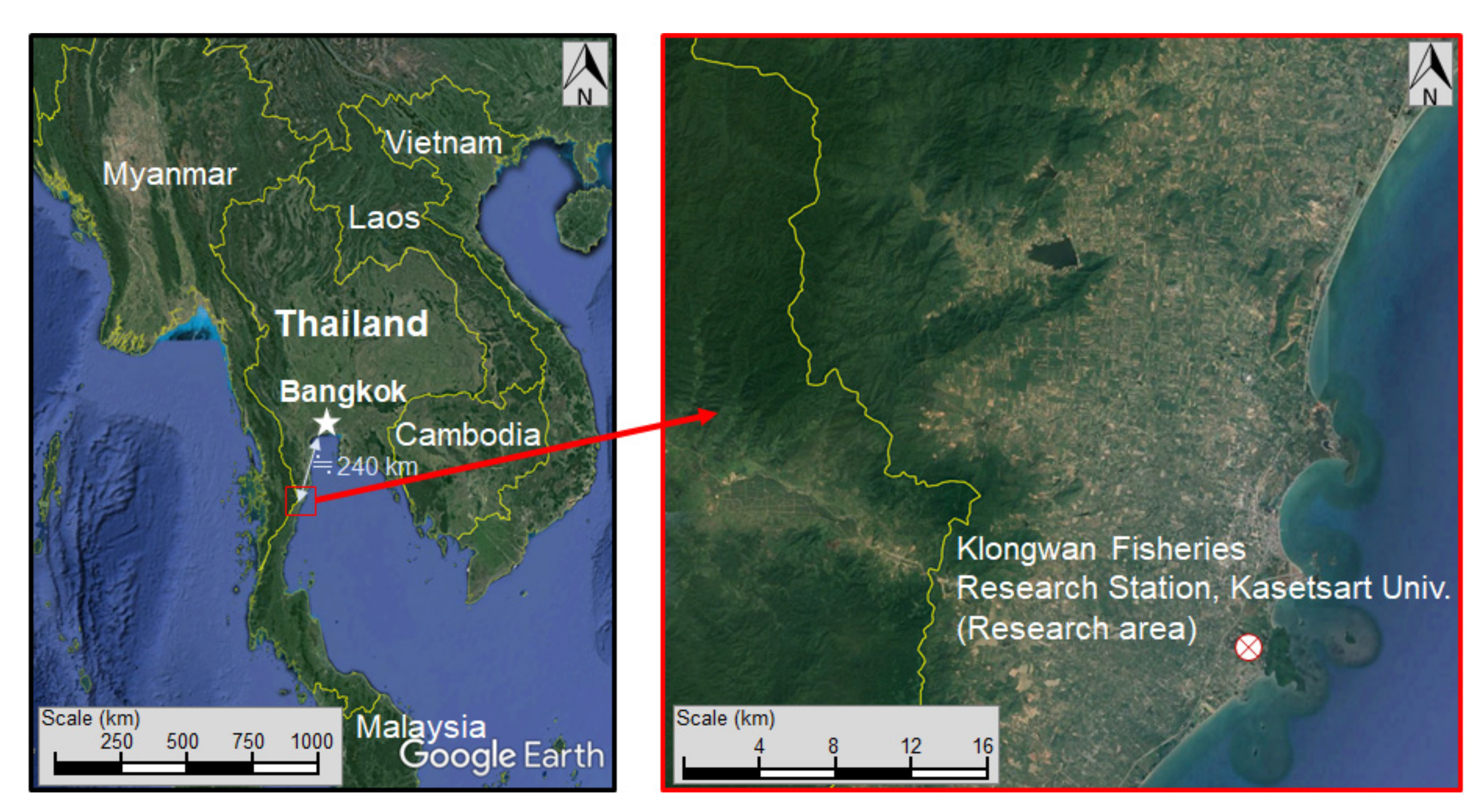
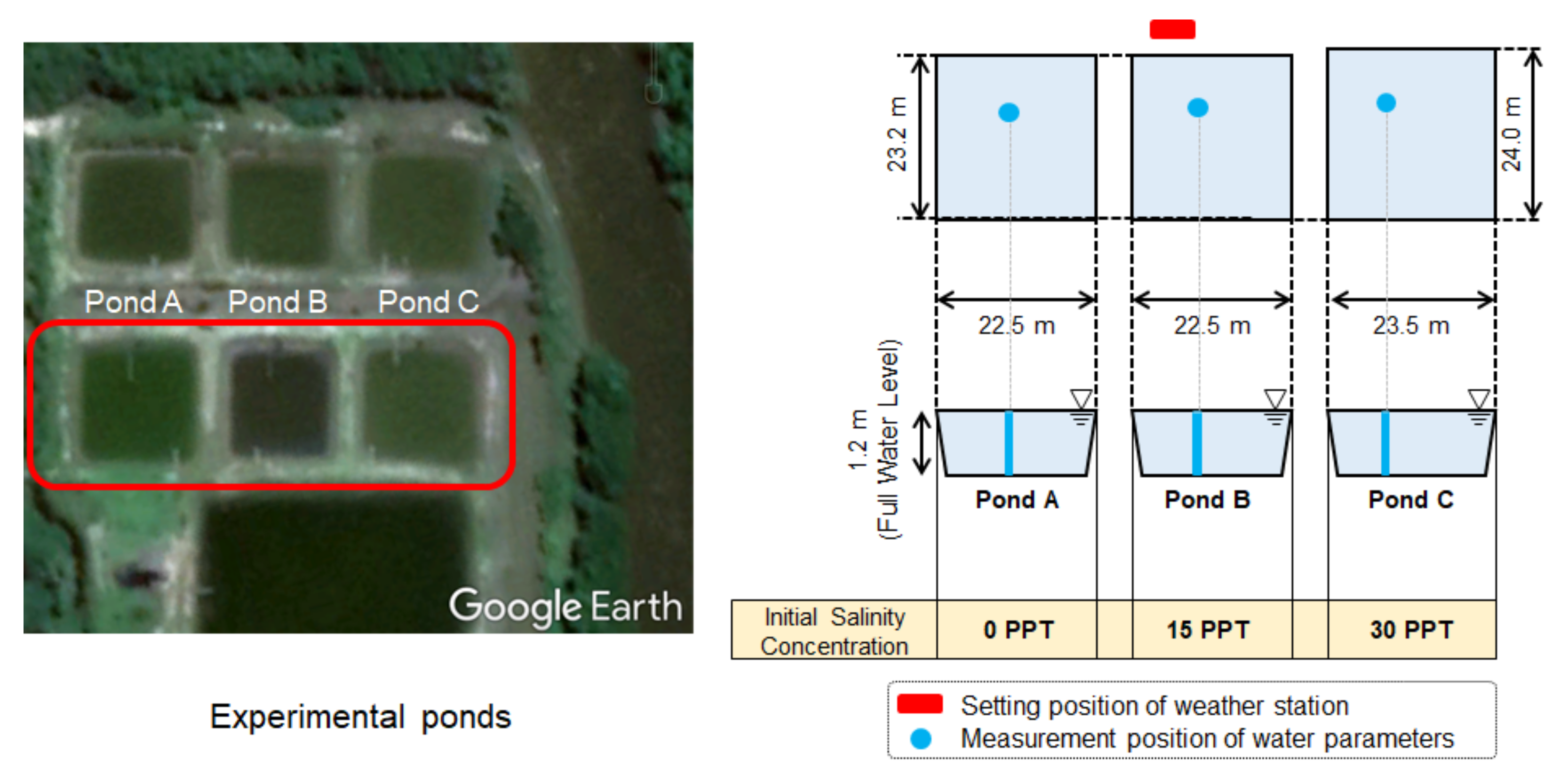
2.1. Study Site and Pond Conditions

Continuous on-site observation was conducted at the experimental aquaculture ponds of the Kasetsart University Khlongwan fishery research station in Thailand (N 11°45′18′′, E 99°47′33′′; Figure 1). Three ponds of similar scale were prepared, in order to investigate the possible differences of halocline formation in different salinity conditions. Salinity conditions were set using seawater and tap water before starting the continuous observation. During the observation period, the salinity and water level were adjusted only once before starting the observation. Therefore, the variation of the salinity and water level depended on the weather conditions. Moreover, the monitoring was conducted without aquaculture products or an aeration system. Therefore, the outcomes of the present study should demonstrate the basic physical phenomena in saline ponds induced by halocline triggered by rainfall in the tropics.

2.2. Monitoring of Pond Environment

In the observations, the time-series variation of the weather and water quality parameters were measured from 1 June to 31 October 2018. This period was the rainy season at the observation location. Figure 2 shows the schematic of the ponds and setting position of sensors for observation, and Table 1 shows the conditions of the measurement parameters. The weather parameters were measured at the edge of Pond B using HOBO weather station (Onset Computer Corporation, Bourne, MA, USA). The setting point of weather station was indicated by the red rectangle in Figure 2. The sensors for ambient temperature, humidity, solar radiation, and rainfall amount were set at 1 m above ground level. The sensors for wind velocity and wind direction were set at 2 m above ground level.
The physical water quality parameters were measured automatically or manually, depending on the parameters. Water temperature, electric conductivity, and pressure at the bottom were automatically measured at 10 min intervals by using Onset HOBO water monitoring data logger series (Onset Computer Corporation, Bourne, MA, USA), which were embedded in a chlorinated polyvinyl chloride pipe. This polyvinyl chloride pipe was mounted in each pond, indicated by the blue circle in Figure 2. The vertical embedding positions for the water temperature sensors were 0.0 m, 0.2 m, 0.3 m, 0.5 m, 0.6 m, and 0.8 m from the bottom, while those for the electric conductivity sensors were 0.1 m, 0.4 m, and 0.7 m from the bottom (i.e., at 0.3 m intervals). As the electric conductivity sensor had the function of water temperature measurement, the water temperature measurement intervals in the vertical direction were 0.1 m, from the bottom to 0.8 m. In addition to these embedding positions, water temperature and salinity sensors were set with a floating body, which could fix the measurement depth at 0.05 m below the water surface, such that the surface water temperature was also measured along with changes in the water level. The mounting position of the pressure sensor was the bottom of the pond. This sensor measured the absolute pressure at the bottom and this pressure data was used for the calculation of water level fluctuations, using the following equation:
H = P w P a / ρ w × g ,
where H is the water level (m), P w is the absolute pressure at the bottom (kPa), P a is the atmospheric pressure (kPa), ρ w is the density of water (kg/m3), and g is the gravitational acceleration (m/s).
On the other hand, Dissolved Oxygen (DO), pH, Turbidity, and Oxidation–Reduction Potential (ORP) were measured using multiple water quality probes (Horiba U50 Water Quality Checker (Horiba Ltd., Kyoto, Japan)), almost five times per week. The measurement positions of these parameters were near the embedding positions of the water temperature and electric conductivity sensors, and the vertical distribution of each parameter was measured at a 0.1 m interval from the bottom to the water surface. As this multiple water quality probe could measure water temperature and salinity, the automatically measured water temperature data were calibrated with the water temperature data of the multiple water quality probe, and the automatically measured electric conductivity (μS/cm) data were converted into salinity (PPT: parts per thousand) using the salinity data of the multiple water quality probe.
In the present study, data observed from 11 July to 31 August were used to assess the impact of haloclines on physical water quality.

2.3. Data Analysis

The observation data were analyzed and plotted using the MATLAB 2020b software, with the Signal Processing Toolbox and Statistics and Machine Learning Toolbox. To detect the start/end day and time of heat storage due to halocline insulation, the “findchangepts” function in the Signal Processing Toolbox was applied to the water temperature time-series data. To clarify the correlation of the parameters, the “pca” function in the Statistics and Machine Learning Toolbox was used, and principal component analysis was conducted using weather and physical water quality parameters.

3. Results and Discussions

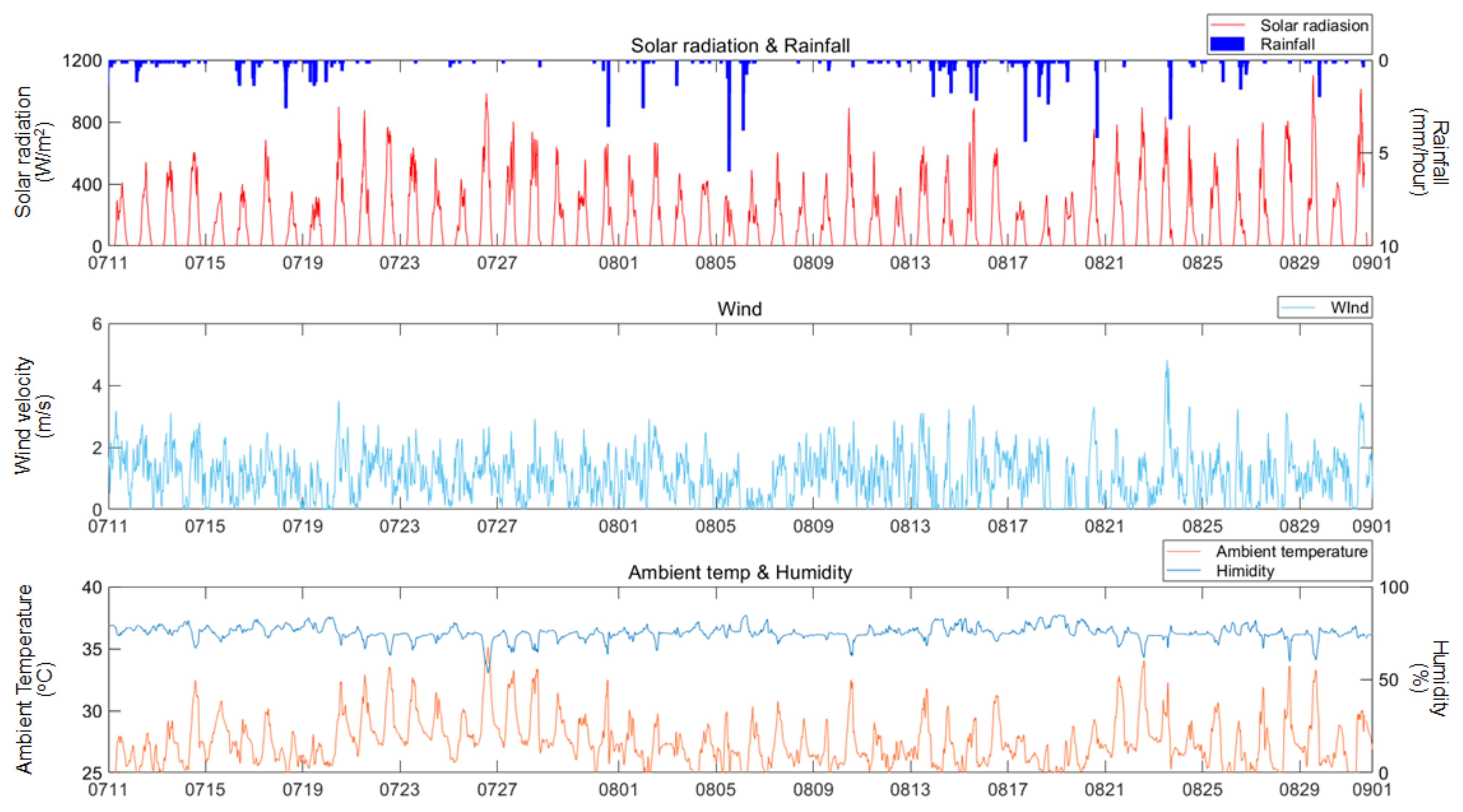
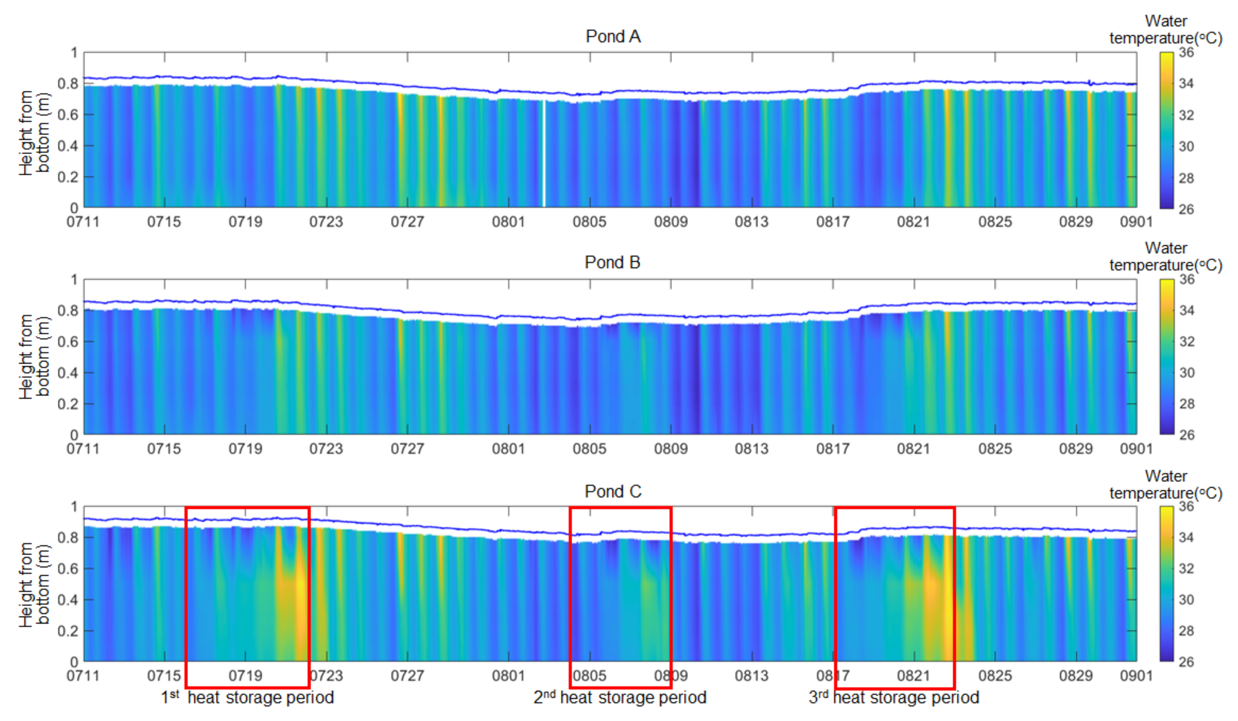
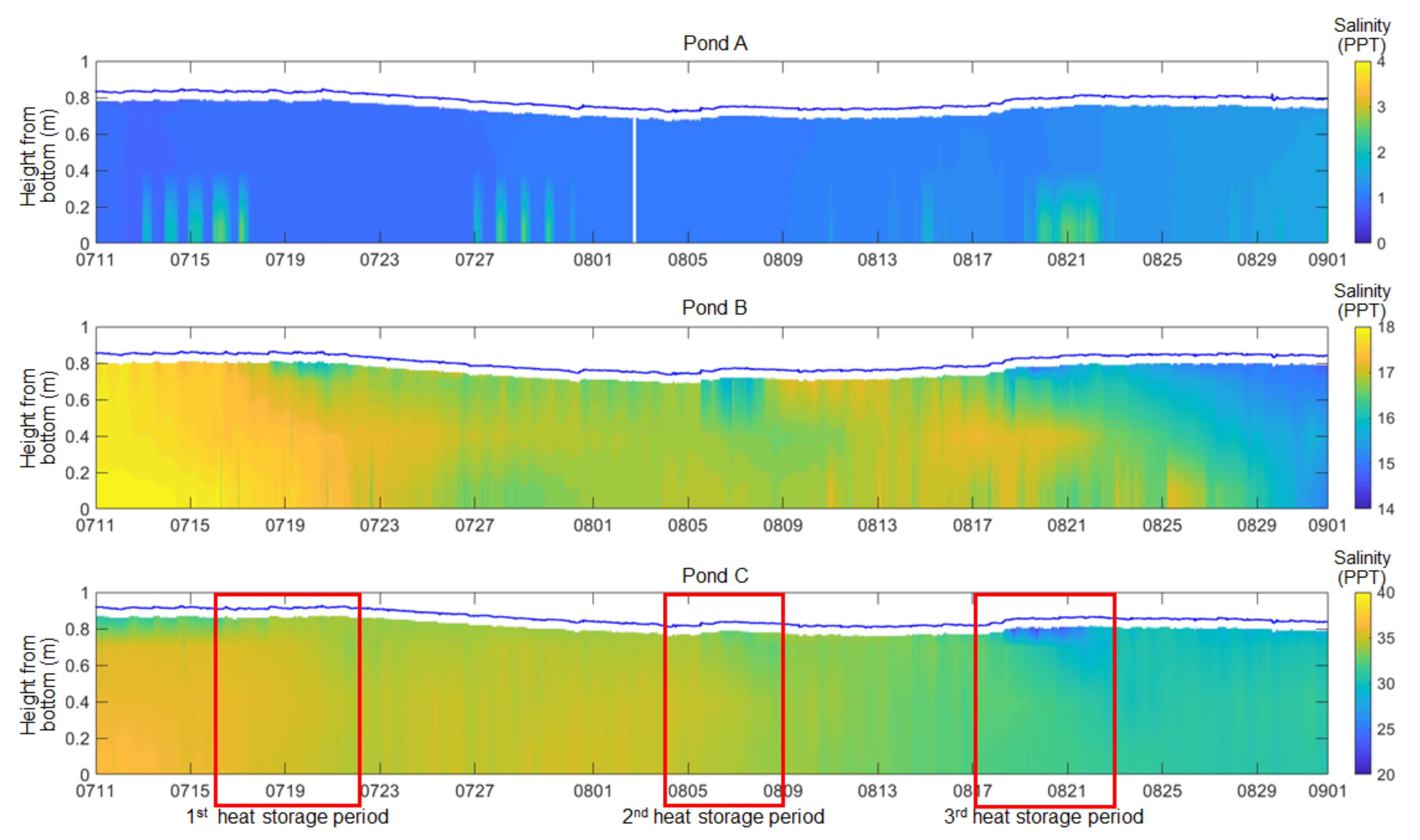
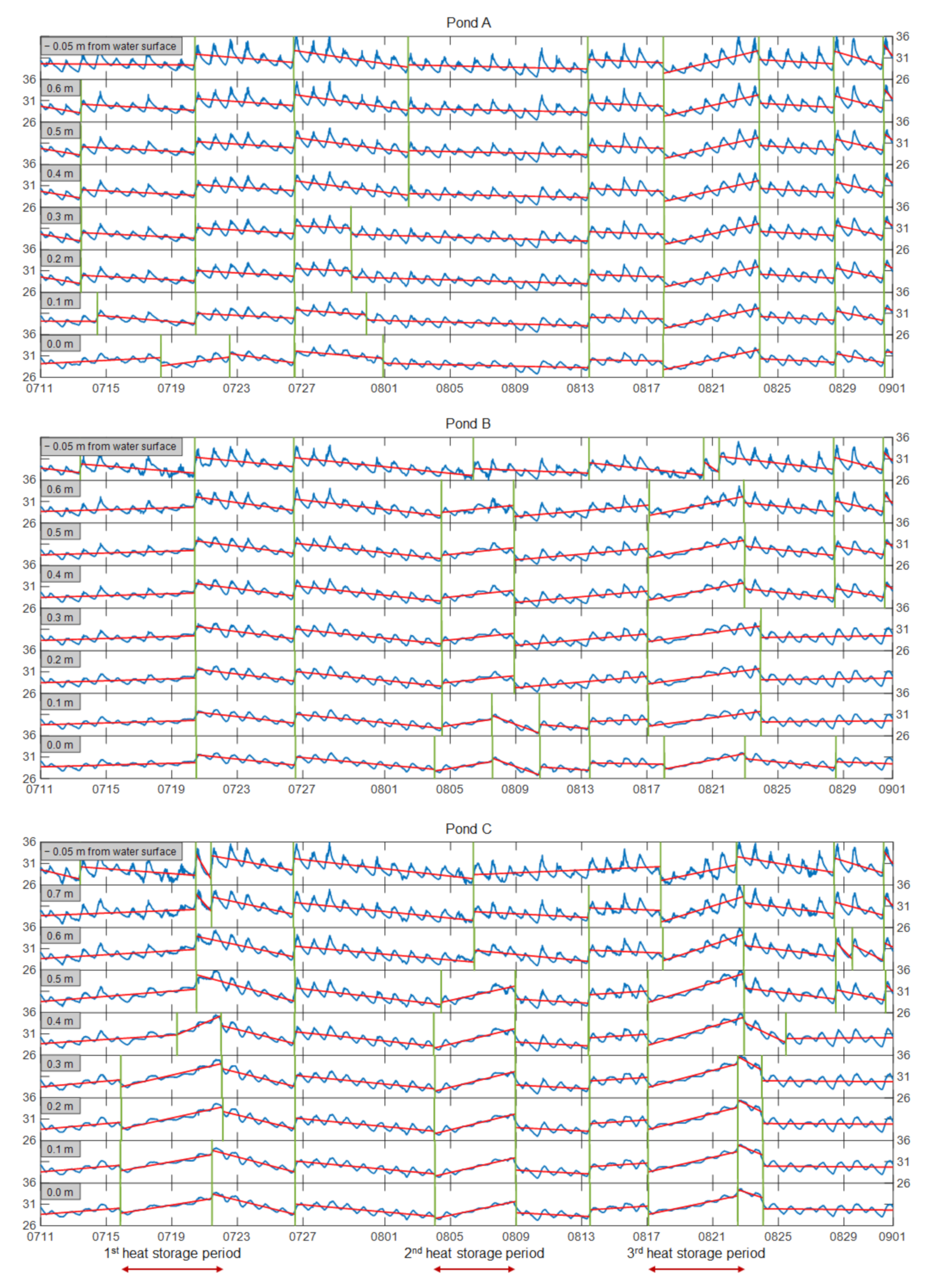
3.1. Variation of Weather, Water Temperature, and Salinity

Figure 3, Figure 4 and Figure 5 illustrate the time-series variation of weather conditions, water temperature, and water salinity in each pond, respectively. In Figure 4 and Figure 5, the contour diagram shows the water temperature and salinity in color. The vertical axis of the contour diagram indicates the distance from the bottom of the pond. In the present observation, as the water temperature and salinity sensors were mounted inside the water body, the distance from the bottom was used as the basic metric for the height. In addition, as the surface water temperature and salinity were also measured with the floating body, the surface water temperature and salinity are also displayed with water level fluctuation.
From Figure 4, it can be clearly seen that high water temperature, from the bottom to middle height, continued for several days in Pond C. This unique variation pattern of water temperature is defined in the present study as “heat storage” in a saline water pond. The heat storage phenomenon in Pond C occurred three times (1st period, 2nd period, and 3rd period, respectively), indicated by the red rectangle in Figure 4 and Figure 5. The definitions of these three periods are given in the following section. From Figure 3, continuous rainfall was observed before the appearance of heat storage in Pond C. This rainfall seemed to cool down and make the water temperature distribution uniform in Pond A. On the other hand, only the water temperature in the surface layer was impacted by the rainfall, while the water temperature in the middle and bottom layers was not impacted by rainfall in Ponds B and C. A similar tendency can be seen in Figure 5. Rainfall impacted the salinity distribution in the vertical direction in Ponds B and C, indicating that low-temperature, lightweight water due to rainfall was floating on the water surface, as salinity differences were formed in Ponds B and C. Incidentally, the salinity concentration in the middle to bottom layers of Pond A increased during several days and periods. This was considered to be due to seawater intrusion from the surrounding canals.
Regarding the tendency of water temperature variation in Pond C, in the 1st and 3rd periods, when the solar radiation was powerful after the continuous rainfall, high water temperatures were continuously observed in Pond C. In contrast, in the 2nd period, when the solar radiation was not intense after the continuous rainfall, the water temperature was not high compared to the other periods. In these three periods, a general daily water temperature cycle induced by solar heating in the day-time and radiative cooling at night-time was observed in Ponds A and B. On the other hand, in Pond C, the water temperature, except for in the surface layer, dramatically increased and seemed not to be affected by radiative cooling at night-time. The maximum water temperature recorded in each heat storage period in Pond C was 36.0 °C at 16:10 on 21 July in the 1st period, 32.8 °C at 18:30 on 7 August in the 2nd period, and 35.9 °C at 16:00 on 22 August in the 3rd period. All of the maximum values were observed at 0.5 m from the bottom. The water temperatures observed in Ponds A and B at the same time and height were as follows: 33.1 °C, 30.0 °C, and 34.3 °C in Pond A, and 32.9 °C, 30.7 °C, and 33.0 °C in Pond B, respectively.

3.2. Classification of Heat Storage Period and Non-Heat Storage Period by Change Point Analysis

As described in the previous section, three different periods were found to be heat storage periods, due to the water temperature variation in Pond C. In order to elucidate the differences in physical water quality parameters between the non-heat storage period and heat storage period, a clear definition of the start and end times of the heat storage period is necessary. In the present study, change point analysis, which can detect distributional changes in time-series data [24,25], was used to define the start and end times of the heat storage period. This analysis was performed in MATLAB, using the function “findchangepts”. For the “findchangepts” function, ‘Statistic’ was specified as ‘linear’, which could enable detection of the changes in the mean and slope, and the ‘maximum number of changes’ was set to nine [26].
Figure 6 shows the results of the change point analysis for the water temperature of each pond. As continuous time-series data are required for change point analysis, the measurement points at 0.7 m in Ponds A and B, which were temporarily exposed in the air due to water level fluctuations, were excluded from the change point analysis. From the results of the change point analysis for Pond C, the start and end dates and times for each heat storage period could be estimated by focusing on the tendency of differences in the slopes associated with Ponds A and B. When the heat storage started in Pond C, the water temperature in the lower layers increased without the impact of radiative cooling. The start time of this water temperature increase can be defined as the beginning of the heat storage phase. On the contrary, as the heat storage phase began to end, the slope of the temporal temperature variation (red line in Figure 6) changed from positive to negative, indicating elimination of the stored heat. This timing can be used to define the end of the heat storage phase. By considering the characteristics of the water temperature variation from the bottom to the middle layer in Pond C, the start and end times of the heat storage phases were defined using the earliest time of water temperature increase and the latest time of water temperature decrease, respectively. In the present study, the period from the start to end of heat storage (in terms of day and time) in Pond C was defined as a “heat storage period”, while the other period was defined as a “non-heat storage period”. Therefore, the whole observation term was divided into three heat storage periods and four non-heat storage periods. The classification information is summarized in Table 2. The following discussions follow this classification.

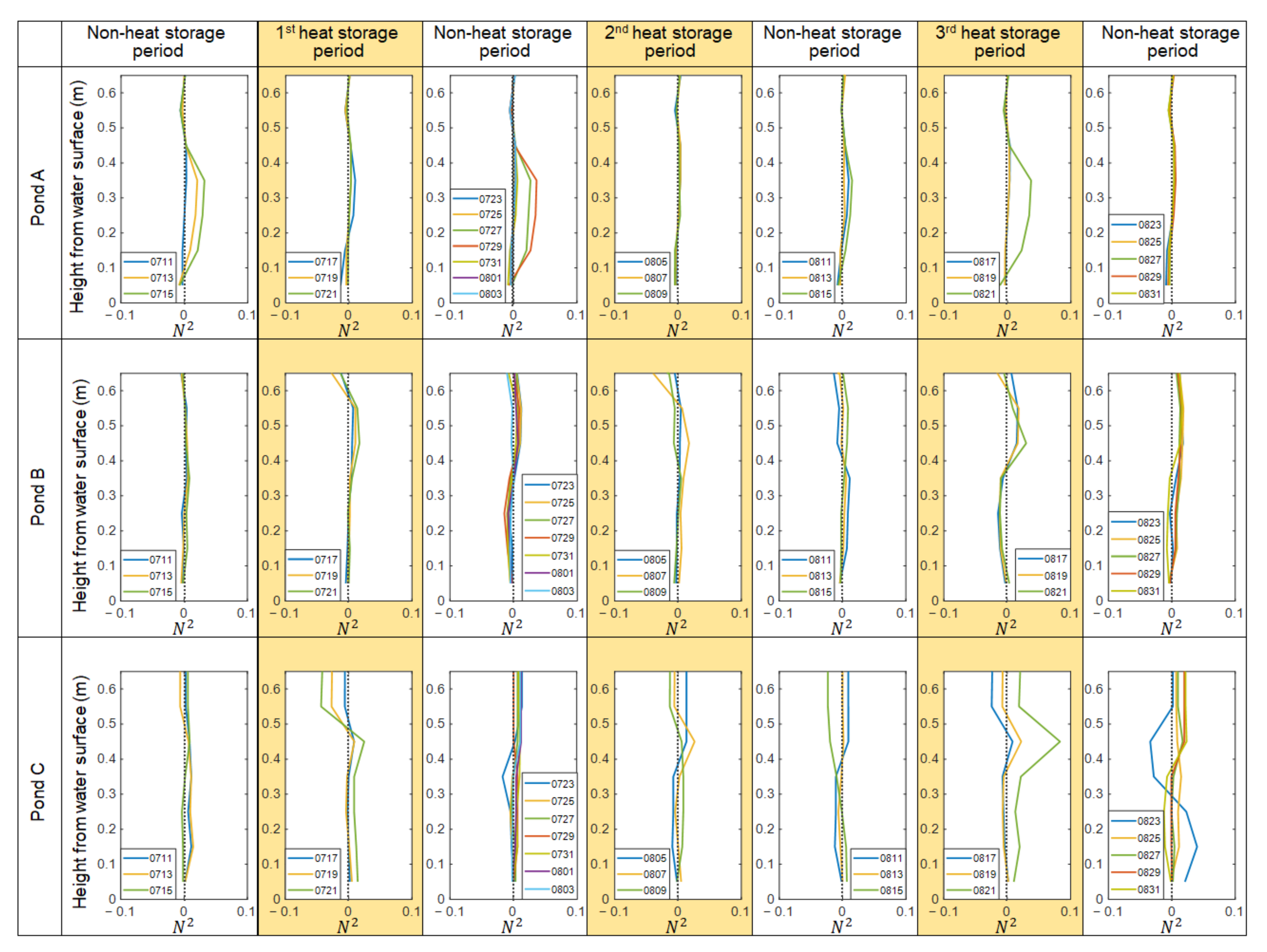
3.3. Structure of Density Stratification

In order to verify the structure of density stratification formed by water temperature and salinity, the Brunt–Väisälä frequency, N 2 N 2 , which is expressed as in Equation (2), was introduced:
N 2 = g ρ r d ρ d z ,
where g is the gravitational acceleration (m/s), ρ r is the reference density (kg/m3), and d ρ / d z is the vertical gradient of water density. The equation proposed by El-Dessouky and Ettouny [27] was applied for calculation of the water density. N 2 is a parameter that can express the stability of density stratification—that is, the conditions of density stratification can be judged through use of the following conditions: N 2 > 0 , stable stratification; N 2 < 0 , unstable stratification; and N 2 = 0 , neutral condition. Moreover, as N 2 is expressed by a density gradient, the vertical distribution of N 2 can explain the structural characteristics of density stratification.
Figure 7 shows the vertical distribution of N 2 at midnight (AM 0:00), divided by each period. In Figure 7, the N 2 values near the water surface, which displayed a sensitive variation to weather conditions, were excluded. In pond A, positive N 2 values in the bottom to middle layers were observed on several days. This was due to seawater intrusion from the surrounding canals, as explained in the previous section. Except for these seawater intrusion days, the N 2 was almost zero from the bottom to the water surface in each period, indicating that the structure of density stratification was neutral, without vertical density differences. On the other hand, in Ponds B and C, the vertical distribution of N 2 had different characteristics between non-heat storage periods and heat storage periods. In non-heat storage periods, N 2 differences for vertical direction were slight and stable in both Ponds B and C, except for the immediate day at the end of heat storage. Therefore, the density stratification was neutral in both Ponds B and C. However, in heat storage periods, the stable value of N 2 was only from the bottom to 0.35 m, while the layer upward of 0.35 m had different variations in Ponds B and C. In Pond B, the N 2 value upward of 0.35 m had positive values without significant differences in the vertical direction, and shifted to a negative value or zero near the water surface. This indicated that the density structure during heat storage periods in Pond B consisted of two layers: a stable density layer with constant salinity concentration from bottom to 0.35 m and a density gradient layer from 0.35 m to the surface. In pond C, the N 2 value upward of 0.35 m had a positive peak value at 0.45 m and a constant value from 0.55 m to the surface. These indicated that the density structure during heat storage periods in Pond C was comprised of three layers: a stable density layer with constant salinity from the bottom to 0.35 m, a halocline with high gradient from 0.4 m to 0.5 m, and a density gradient layer with low salinity from 0.5 m to the water surface.
Regarding the function of the solar pond, as mentioned in the previous section, when the salinity stratification is stratified into three layers with a lower high-salinity layer, a middle halocline, and an upper low-salinity layer, the halocline layer has an insulation effect on both the lower and upper layers [4,5,6,7,8]. From the N 2 distribution in the vertical direction, the heat storage in Pond C showed a similar phenomenon as that with solar ponds (i.e., with the formation of salinity stratification due to rainfall, the salinity conditions led to stratification into three layers). As a result, the heat was stored in the lower high-salinity layer, due to the halocline insulation effect. This effect suppressed both heat loss from the lower high-salinity layer and radiative cooling at night-time. Therefore, the heat storage layer could be considered from the bottom to 0.4 m in each heat storage period in the observed data. In the following section, the lower high-salinity layer and the upper layer are distinguished, in order to explain the physical water quality characteristics.

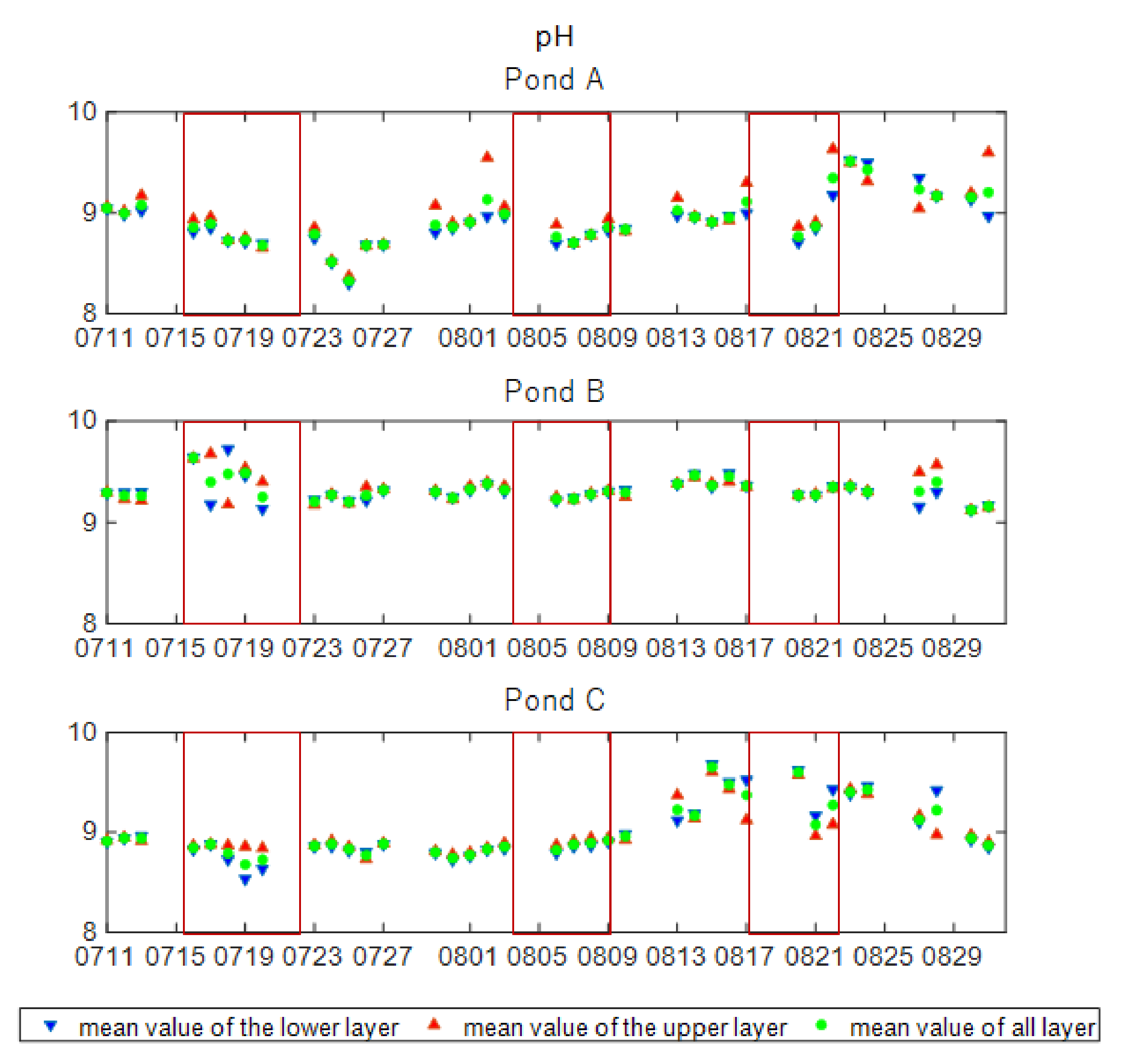
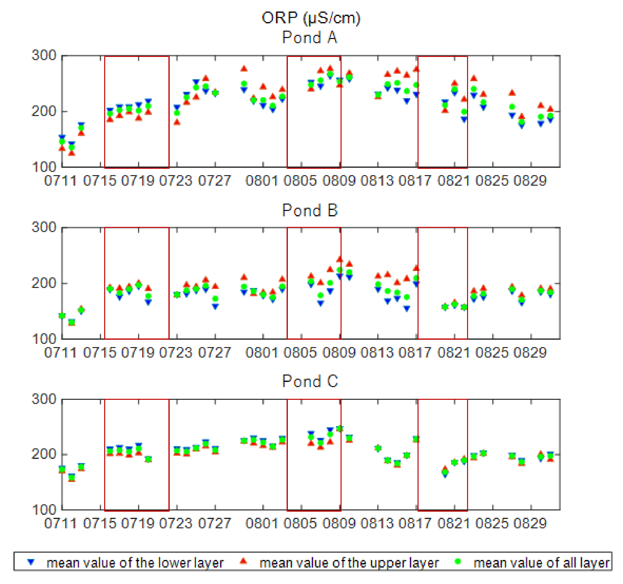
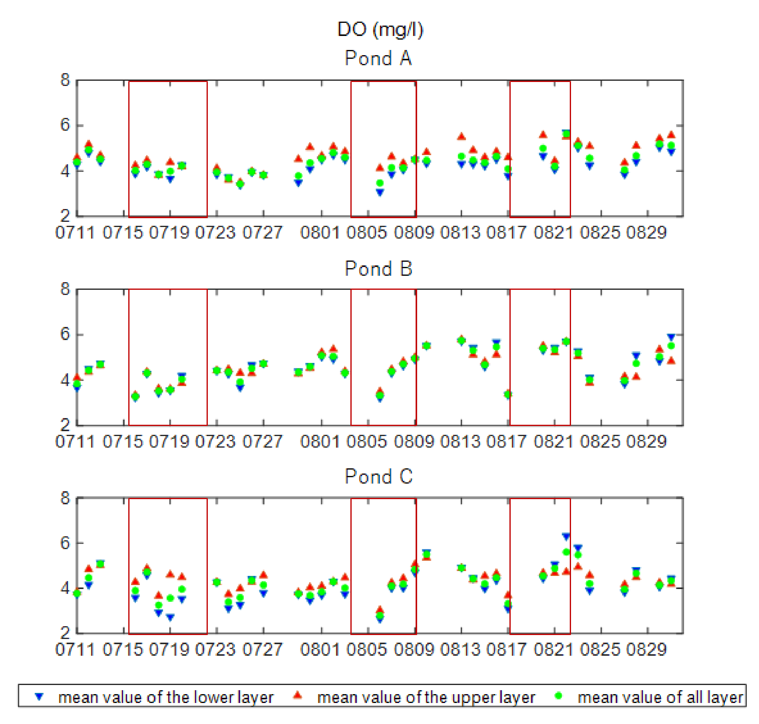
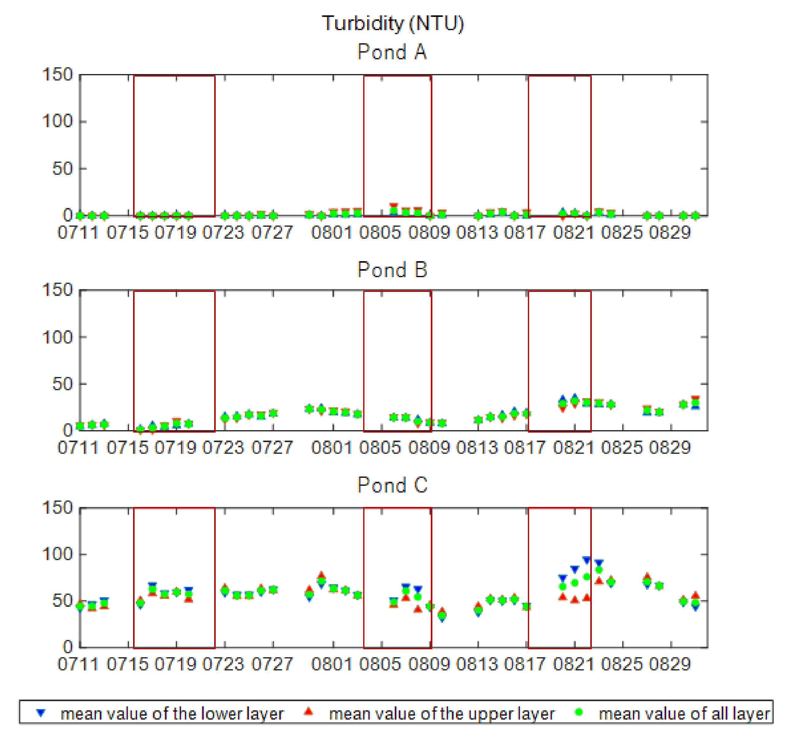
3.4. Characteristic Physical Water Quality Variation Divided into the Periods and Layers

In the above section, the observation period was divided into two periods: the heat storage period and the non-heat storage period. Moreover, the layer from the bottom to 0.4 m was characterized as having the function of heat storage. Therefore, to consider the impact of the halocline on the physical water quality parameters, it would be reasonable to divide the parameters into periods and layers.
Figure 8, Figure 9, Figure 10 and Figure 11 show the mean of DO, pH, Turbidity, and ORP variation in the lower layer (blue inverted triangle), the upper layer (red triangle), and all layers (green circle), respectively. The red rectangles indicate the heat storage period in Pond C. In the observation ponds, DO variation was affected by O2 consumption due to the respiration of micro-organisms, and O2 production by photosynthetic phytoplankton or supplemented by reaeration at the water surface. pH variation was mainly impacted by the biological and chemical reactions that release or consume CO2. The main component of turbidity could be micro-organisms inside the ponds and suspended solids inflowed by rainfall. ORP was affected by the aerobic or anaerobic state of the water.
From Figure 8, the variation tendency of the mean value of DO for all layers was almost similar among the ponds. In Ponds A and C, DO differences in the layers were observed for almost all days. On the other hand, in Pond B, the DO differences in layers were slight. The mean value of DO in the lower layer was lower than that of the upper layer on most observation days. However, for a few days, the mean value of the lower layer was higher than that of the upper layer in Ponds B and C. In heat storage periods, the mean value of DO was increased in all ponds. Especially in the 3rd heat storage period, the increase ratio of mean value of DO in the lower layer was higher than that of the upper layer in Pond C.
From Figure 9, the mean pH differences in layers were slight in all ponds, except for a few days. In pond A, the pH fluctuation range was high, compared with Ponds B and C. Although, in some periods, the pH fluctuation range was high in Ponds B and C, there were no common fluctuation patterns among the ponds. Moreover, the variation of the mean pH value during heat storage periods could not be characterized.
From Figure 10, the mean turbidity value was different in each pond. In Pond A, the mean turbidity value retained a low value, even near the bottom, except for several days after the rainfall event. The reason that the mean turbidity value maintained a low value in Pond A could be attributed to the tap water used for Pond A. As the pond’s location was near the coastal area and the surrounding water environments were of seawater origin, it could be considered that the micro-organisms from the surrounding water bodies could not invade Pond A. In Pond B, the mean turbidity value increased gradually, with several-day increase and decrease periods. The mean value was low on 11 July. However, on 31 August the value was 30. The increase or decrease ratio of turbidity was almost constant during each increase or decrease period, respectively. In Pond C, the mean turbidity value kept an almost constant range until 7 August, then decreased until 9 August. After 9 August, the value increased until 23 August and again converged around 50. In heat storage periods in Pond C, the mean value of the lower layer was higher than that of the upper layer in Pond C. Especially in the third period of heat storage in Pond C, the increase ratio for the mean value of the lower layer was high.
From Figure 11, the variation tendency of the mean ORP value in all layers was almost similar among the ponds. However, there were differences in the layers of Ponds A and B, while there was little difference in the layers of Pond C. The mean ORP value of the lower layer was lower than that of the upper layer in Pond B, while the mean value of the lower layer of ORP was higher than that of the upper layer for several days in Ponds A and C. However, the variation of the mean ORP value during heat storage periods could not be characterized. As significant fluctuation was not observed through the observation period, it could be considered that there was no rapid deterioration of water quality accompanied by anaerobiosis.

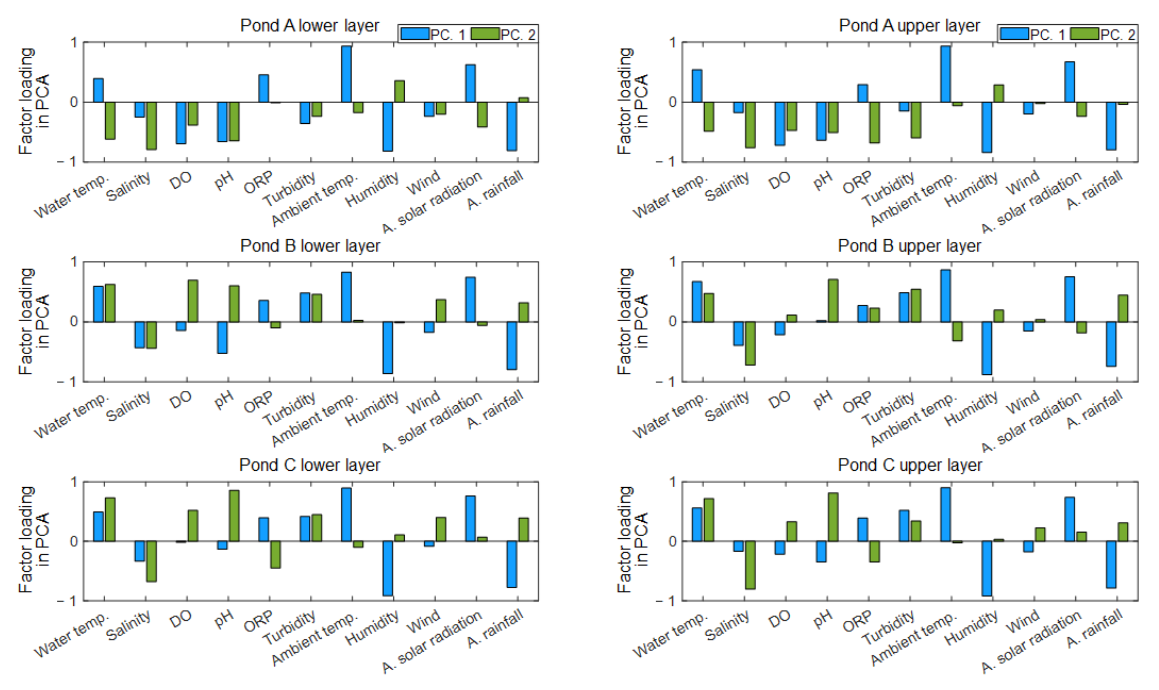
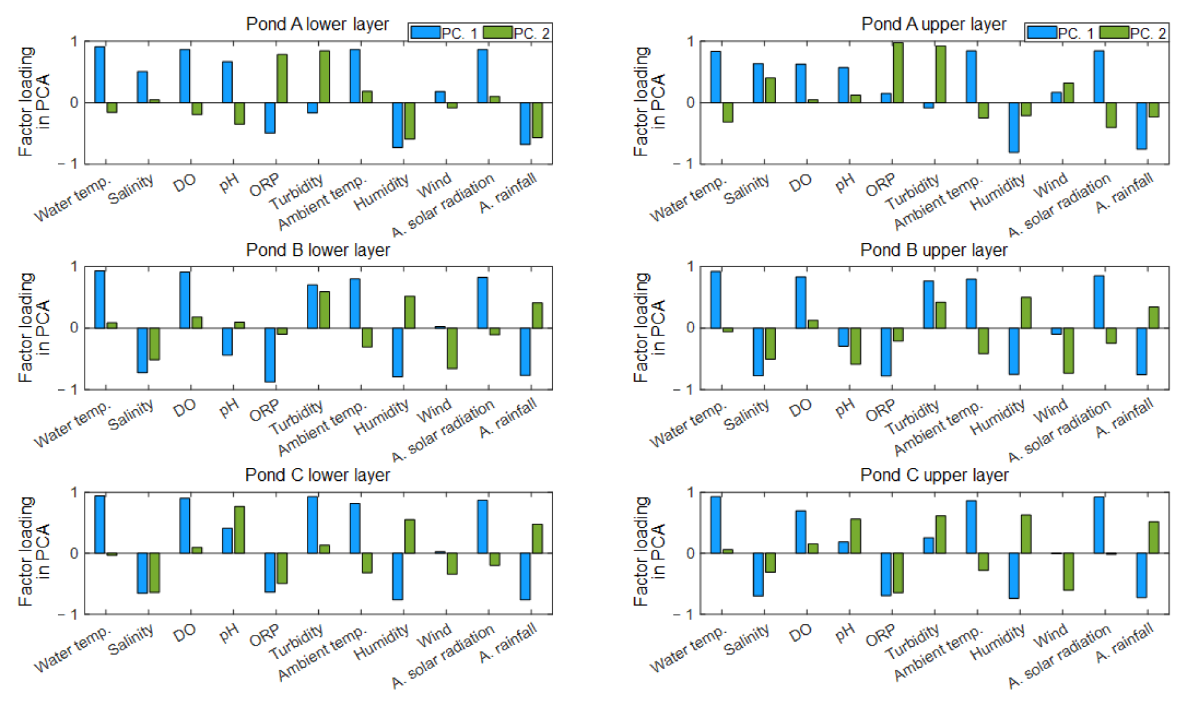
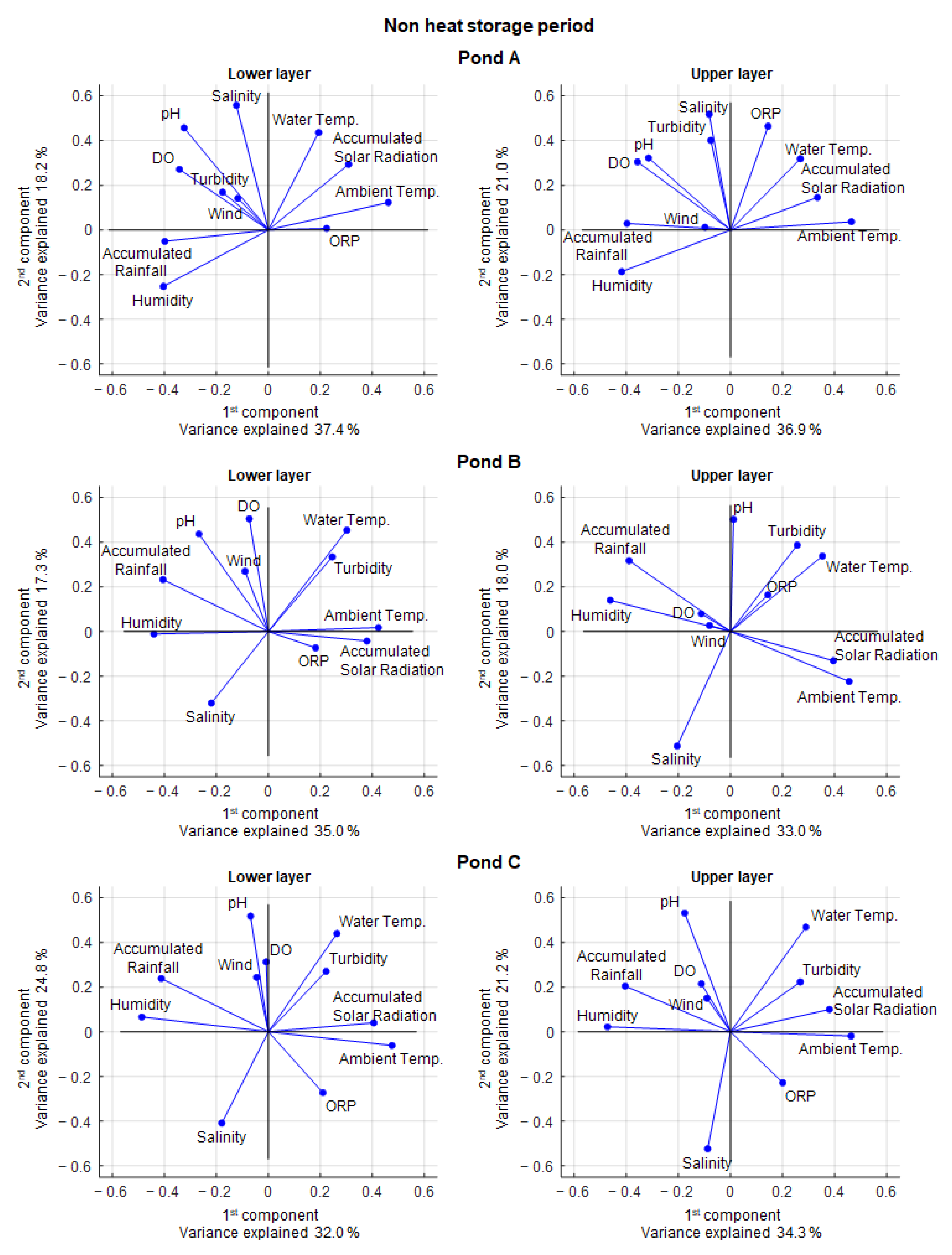
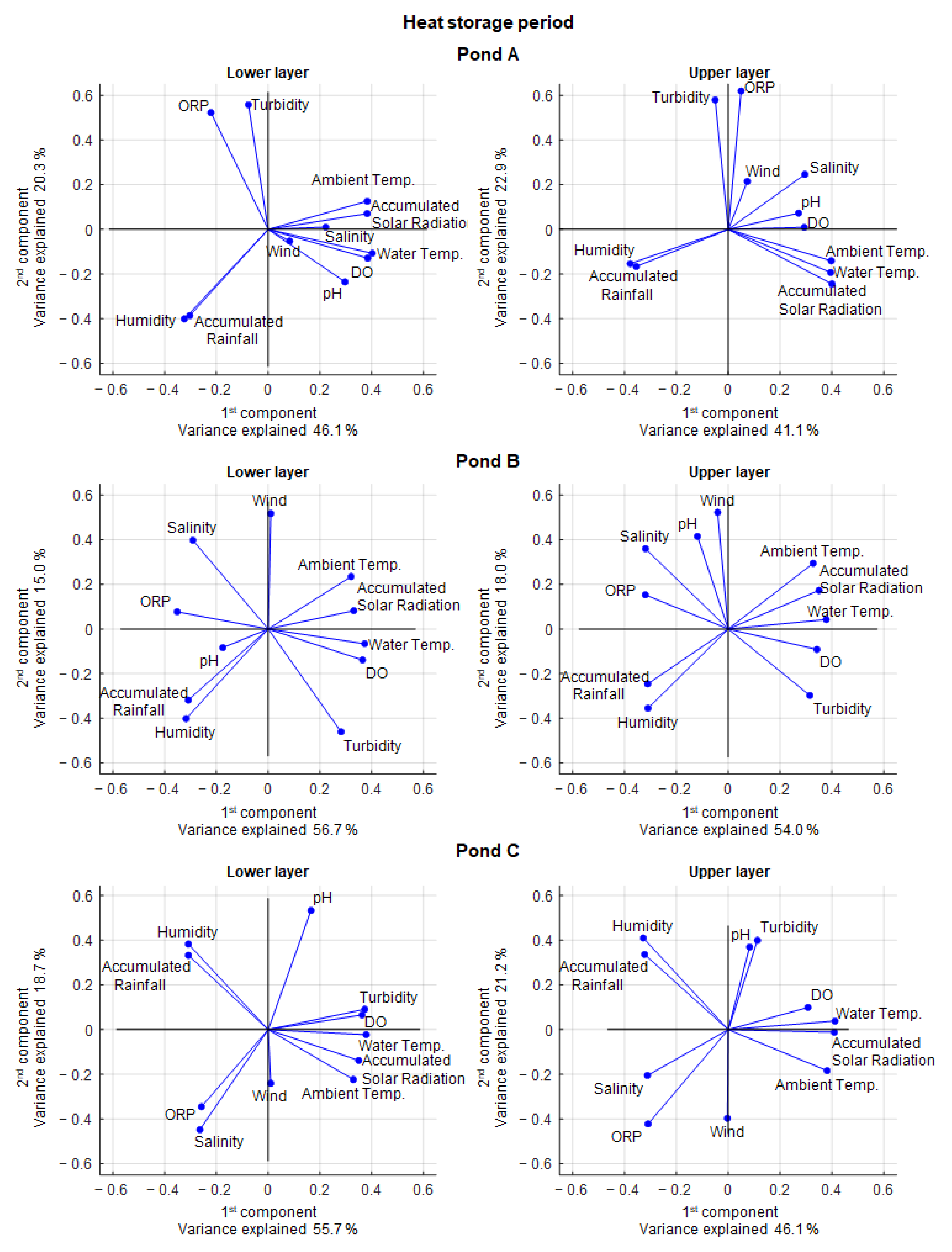
3.5. Princpal Component Analysis for Observed Parameters

In order to verify the correlation of the observed parameters between specific periods and layer differences, principal component analysis (PCA) was applied. PCA is a technique for reducing the dimensionality of data sets, increasing interpretability, and minimizing information loss [28]. Its goal is to extract critical information from the data, represent it as a set of new orthogonal variables called principal components, and display the correlations between the observations [29].
For the application of PCA, weather variation parameters and physical water quality parameters obtained by the multiple water quality probe were used, and the following data processing steps were applied: (1) all of the measurement parameters were divided into the two-period classification (heat storage period and non-heat storage period) by following the results of change point analysis; (2) as the manual measurements of physical water quality parameters were conducted five times per week, the weather parameters—corresponding to the timing of the manual measurements—were averaged (ambient temperature, humidity, and wind) and accumulated (solar radiation and rainfall), ranging from the previous to the latest measurement period (e.g., the previous observation: 23 July, 12:40; and the latest observation: 24 July, 12:30 for physical water quality measurements; the mean/accumulation value for 24 July was obtained from 23 July, 12:40 to 24 July, 12:30); (3) the water quality parameters were divided into two layers: bottom to 0.4 m (lower layer) and 0.5 m to 0.05 m below from the water surface (upper layer) in each pond; (4) the normality of data was tested using the Anderson–Darling test [30] and, in the case that the obtained data set did not follow the normal distribution (p-value < 0.05), log-transformation was applied to the data set [31]. The descriptive statistics of weather and water quality parameters in each pond, calculated through the above data processing steps, are summarized in Table 3 and Table 4, respectively.
From Table 3, it can be seen that there were no significant differences in ambient temperature, humidity, and wind; however, there were differences in accumulated solar radiation and rainfall between the non-heat storage period and the heat storage period. This suggests that the heat storage period included more cloudy or rainy periods than non-heat storage periods. Moreover, it was also found that the rainfall in heat storage periods did not fall in the manner of a strong storm. In Table 4, brief tendency differences between the non-heat period and heat storage period or upper and lower layers can be observed. For instance, the mean value of water temperature for the non-heat storage period was lower than that for the heat storage period (except for Pond A), while the mean DO value for the upper layer was higher than that of the lower layer for each period. However, the correlations among water quality and weather parameters were not clearly revealed.
Table 5 shows variance explained and cumulative variance explained for first to fifth principal components (PCs). The variance explained indicates how much of the data (in percentage) can be explained by the PCs. According to previous studies on PCA, the appropriate range of cumulative variance explained by the PCs depends on the researcher. For instance, Hair et al. [32] suggested 60%, while Jolliffe and Cadima. [28] suggested 70% for the cumulative variance explained. Therefore, if we verified the correlations between all parameters observed in the present study by PCA, it must be reasonable to consider the first to third or fourth principal components for the scope of verification; however, as one of the essential impacts of the halocline on physical water quality is heat storage, the first and second PCs, which had high factor loading for water temperature, are discussed in the PCA summary.
Figure 12 and Figure 13 indicate the factor loadings by first and second PCs for the non-heat storage period and heat storage period, respectively. The factor loading indicates the contribution of obtained parameters to each PC. If the value of factor loading is close to −1 or 1, the parameter has an intense contribution to the PCs.
Figure 12, for the non-heat storage period, shows that the dominant parameters in PC 1 were weather variation, ambient temperature, accumulated solar radiation, humidity, and accumulated rainfall in each pond and both layers. On the other hand, the dominant parameters in PC 2 were water quality variation; however, the factor loading rank differed among the ponds and layers. The factor loading of water temperature in the lower layer of three ponds in the non-heat storage period was comparatively low, indicating a low correlation with the ambient temperature and solar radiation. In addition, the value of variance explained (shown in Table 5) was comparatively low, ranging from 32.0% (Pond C, Lower layer) to 37.4% (Pond A, Lower Layer) in PC 1, and from 17.3% (Pond B, Lower Layer) to 24.9% (Pond C, Lower Layer) in PC 2. This indicates that the variation of the obtained parameters in the non-heat storage period was dominated by multiple factors with incoherent variation patterns. On the other hand, from Table 5, for the heat storage period, the value of variance explained in PC 1 was higher than that for the non-heat storage period in each pond and layers, ranging from 41.1% (Pond A, Upper Layer) to 56.7% (Pond B, Lower Layer). Therefore, it could be considered that the variation of the obtained parameters in the heat storage period had a comparatively higher correlation with parameters than those of the non-heat storage period.
From Figure 13, for the heat storage period, the dominant parameters in PC 1 were not only weather parameters, but also water quality parameters. Moreover, the factor loading for water temperature in PC 1 was high in each pond and period, such that the variation of water temperature contributed to the variation of water quality parameters. The other high values of factor loadings associated with water quality in PC 1 differed among the ponds. In Ponds A and B, the high factor loading values were DO and pH in Pond A, as well as DO and turbidity in Pond B, while differences in layers could not be found in both ponds. On the other hand, in Pond C, a difference between layers was observed. The high factor loading values associated with water quality in Pond C were DO and turbidity in the lower layer, but only DO in the upper layer. This indicated that DO and turbidity in the lower layer of Pond C, which had heat storage, could increase with the water temperature.
To obtain a more evident correlation among the parameters analyzed by PCA, biplots for non-heat storage period and heat storage period are shown in Figure 14 and Figure 15, respectively. As detailed explanations of Figure 14 and Figure 15 would overlap with the explanations of Figure 12 and Figure 13, the explanation and discussion of Figure 14 and Figure 15 focus on the relationships between water temperature, DO, and turbidity.
From Figure 14, for the non-heat storage period, the PCA scores of water temperature, DO, and turbidity in Pond A had similar distribution between the lower and upper layers. However, each distribution had differences, and their correlation was low. On the other hand, water temperature and turbidity in Ponds B and C were in the same quadrant for both layers, and only DO was distributed in a different quadrant. Therefore, it could be considered that the variation of water temperature and turbidity had high correlation.
On the other hand, as can be seen from Figure 15, for the heat storage period, the PCA scores of water temperature and DO had similar distributions, and these parameters were correlated in each pond and layer. In Pond A, for which the turbidity was low, the PCA score of turbidity was different from those of water temperature and DO in each layer. In Pond B, the PCA scores of water temperature, DO, and turbidity were distributed closely in each layer, which indicated that an increase in water temperature contributed to an increase in turbidity, with the same mechanism as explained above. In addition, as the positions of turbidity and DO were comparatively close, one of the significant components of turbidity could be conjectured as phytoplankton. In Pond C, the PCA scores of water temperature, DO, and turbidity were distributed relatively closely in the lower layer when heat storage occurred, while turbidity was distributed farther away from water temperature and DO in the upper layer. Therefore, the water quality conditions were different between the lower and upper layers during heat storage periods in Pond C.

3.6. Mechanism of Different Water Quality Conditions during Heat Storage Period in Pond C

From the discussion of PCA results, the water quality condition differences between the lower heat storage layer and the upper layer could be characterized by the difference in turbidity conditions. In this section, the considerable mechanism of turbidity differences in layers and their impact is discussed.
The controlling factors of turbidity in the considered observation ponds were the inflow of suspended matter by rainfall and increases or decreases in micro-organism populations. When suspended matter inflow by rainfall is the dominant factor of turbidity, the time-series mean value of turbidity in Figure 10 would be expected to increase during or after the rainfall event, and the correlation between turbidity and accumulated rainfall would also be expected to be confirmed in the PCA results in Figure 14 and Figure 15. However, these findings were not obtained. Therefore, the dominant factor of turbidity, especially in the saline ponds (B and C), can be attributed to population changes in micro-organisms during heat storage periods.
The mechanism that changed the turbidity tendency between the lower and upper layers in Pond C could be considered as being due to a halocline associated with the formation of three density-stratified layers induced by rainfall. As mentioned in the previous section, if the three-layer salinity stratification was composed of a lower high-salinity layer, a halocline layer, and an upper low-salinity layer, then the halocline layer would be non-convective and heat storage would progress in the lower high-salinity layer. The mechanism of heat storage in the lower high-salinity layer conveys an insulating effect of heat transfer, due to non-convection in the halocline. As with the mechanism of heat transfer, turbidity movements between the lower high-salinity layer and the upper layer may also be interrupted by the halocline. This interruption of turbidity can be also conjectured through observation of Figure 15. In Pond B, as the three-layer stratification was not formed during heat storage periods and the turbidity movements were not interrupted, the PCA scores of turbidity, temperature, and DO were distributed almost similarly between the lower and upper layers. On the other hand, in Pond C, as the turbidity movements including micro-organisms between the lower and upper layers were interrupted, due to the existence of the halocline, the PCA score of turbidity had a different distribution between the lower and upper layers. These different characteristics of turbidity in Ponds B and C can also be confirmed by the mean values of turbidity shown in Figure 8. These results, which indicate physical water quality differences across the halocline, are similar to those of previous studies by Ueda et al. [1], Jeong and Kwak [9], and Lougee et al. [10], which clarified the characteristic differences, in terms of both water quality and the ecosystem, between the upper and lower layers in brackish water and estuaries. Although these previous studies dealt with haloclines in large-scale water bodies, the present study indicated that the difference in water quality between the upper and lower layers due to the appearance of a halocline can be observed in water bodies as small as aquaculture ponds.

4. Conclusions

In the present study, haloclines triggered by rainfall in saline water ponds were investigated through continuous on-site observation data. Using these data, we successfully observed the halocline and explained the causal mechanism of the phenomenon. In addition, the halocline was suggested not only to cause heat storage, but also to impact turbidity and DO. Our significant findings can be summarized as follows:
  • The important trigger which could induce halocline formation in saline water ponds is rainfall. When rainfall can generate salinity stratification, halocline phenomena may occur in the pond.
  • The condition of salinity stratification was confirmed by the vertical distribution of the Brunt–Väisälä frequency, N 2 , which expresses the stability of density stratification. When a halocline can occur in a water body, the vertical distribution of N 2 has a peak value at the middle height of the pond.
  • The start/end timing of the heat storage could be estimated by change point analysis for the time-series data of the water temperature obtained in the lower layer.
  • When a halocline forms in a saline water pond, heat can be stored in the lower high-salinity layer, due to the halocline insulation effect.
  • With the appearance of a halocline, movements of turbidity, including micro-organisms between the lower and upper layers, are interrupted. As a result, the turbidity and DO distributions can change during the heat storage period.
The results of the present study indicate that the halocline in a saline water pond, triggered by rainfall, may possibly increase the water temperature into a risky range for aquaculture production. Moreover, water quality parameters, such as turbidity and DO, also have the possibility to change with the appearance of the halocline; however, as the present observations only observed the physical water quality parameters that could be measured on-site, detailed water quality parameters, especially those associated with chemicals, could not be assessed. Furthermore, as the objective of the present study was to clarify the basis of the phenomenon associated with a halocline induced by rainfall, the observations were conducted in a situation without aquaculture production. In an actual aquaculture environment, the biological reactions due to aquaculture production and the chemical reactions due to water quality substances could be impacted by a halocline. Therefore, further investigation and consideration, which could clarify the impact of haloclines on whole aquaculture pond components, would be necessary for more critical clarification of the relationships between haloclines and aquaculture production.

Author Contributions

Conceptualization, A.O.; methodology, A.O. and P.K.; validation, A.O., P.K., T.N.V. and M.M.; formal analysis, A.O. and T.N.V.; investigation, A.O. and P.K.; resources, A.O., P.K., T.N.V. and M.M.; data curation, A.O., P.K. and T.N.V.; writing—original draft preparation, A.O.; writing—review and editing, A.O., P.K., T.N.V. and M.M.; visualization, A.O.; supervision, A.O.; project administration, A.O.; funding acquisition, A.O. All authors have read and agreed to the published version of the manuscript.

Funding

This research was funded by CASIO Science Promotion Foundation.

Institutional Review Board Statement

Not applicable.

Informed Consent Statement

Not applicable.

Data Availability Statement

The data that support the findings of this study are available from the corresponding author, upon request.

Conflicts of Interest

The authors declare no conflict of interest. The funders had no role in the design of the study; in the collection, analyses, or interpretation of data; in the writing of the manuscript; or in the decision to publish the results.

References

  1. Ueda, S.; Kondo, K.; Chikuchi, Y. Effects of the halocline on water quality and phytoplankton composition in a shallow brackish lake (Lake Obuchi, Japan). Limnology 2005, 6, 149–160. [Google Scholar] [CrossRef]
  2. Velmurugan, V.; Srithar, K. Prospects and scopes of solar pond: A detailed review. Renew. Sustain. Energy Rev. 2008, 12, 2253–2263. [Google Scholar] [CrossRef]
  3. Date, A.; Yaakob, Y.; Date, A.; Krishnapillai, S.; Akbarzadeh, A. Heat extraction from Non-Convective and Lower Convective Zones of the solar pond: A transient study. Sol. Energy 2013, 97, 517–528. [Google Scholar] [CrossRef]
  4. Hull, J.R.; Nielsen, J.; Golding, P. Salinity Gradient Solar Ponds; CRC press: Boca Raton, FL, USA, 1988. [Google Scholar]
  5. Abdullah, A.A.; Fallatah, H.M.; Lindsay, K.A.; Oreijah, M.M. Measurements of the performance of the experimental salt-gradient solar pond at Makkah one year after commissioning. Sol. Energy 2017, 150, 212–219. [Google Scholar] [CrossRef]
  6. Sukhatme, S.P. Solar Energy: Principles of Thermal Collection and Storage, 4th ed.; McGraw-Hill Inc.: New York, NY, USA, 2017. [Google Scholar]
  7. Verma, S.; Das, R. Wall profile optimisation of a salt gradient solar pond using a generalized model. Sol. Energy 2019, 184, 356–371. [Google Scholar] [CrossRef]
  8. Angeli, C.; Leonardi, E. A one-dimensional numerical study of the salt diffusion in a salinity-gradient solar pond. Int. J. Heat Mass Transf. 2004, 47, 1–10. [Google Scholar] [CrossRef]
  9. Jeong, Y.-H.; Kwak, D.-H. Influence of external loading and halocline on phosphorus release from sediment in an artificial tidal lake. Int. J. Sediment Res. 2020, 35, 146–156. [Google Scholar] [CrossRef]
  10. Lougee, L.A.; Bollens, S.M.; Avent, S.R. The effects of haloclines on the vertical distribution and migration of zooplankton. J. Exp. Mar. Biol. Ecol. 2020, 278, 111–134. [Google Scholar] [CrossRef]
  11. Uurasjärvi, E.; Pääkkönen, M.; Setälä, O.; Koistinen, A.; Lehtiniemi, M. Microplastics accumulate to thin layers in the stratified Baltic Sea. Environ. Pollut. 2021, 268, 115700. [Google Scholar] [CrossRef] [PubMed]
  12. FAO. Fishery and Aquaculture Statistics. 2021 Global Aquaculture Production 1950–2019 (FishstatJ). In FAO Fisheries Division [online]; Rome. Updated 2021. Available online: www.fao.org/fishery/statistics/software/fishstatj/en (accessed on 25 April 2021).
  13. Oddsson, G.V. A Definition of Aquaculture Intensity Based on Production Functions—The Aquaculture Production Intensity Scale (APIS). Water 2020, 12, 765. [Google Scholar] [CrossRef] [Green Version]
  14. Boyd, C.E.; Tucker, C.S. Water Quality Requirements in Pond Aquaculture Water Quality Management; Springer Science & Business Media: Berlin/Heidelberg, Germany, 2012. [Google Scholar]
  15. Walker, P.J.; Winton, J.R. Emerging viral diseases of fish and shrimp. Vet. Res. 2010, 41, 51. [Google Scholar] [CrossRef] [PubMed] [Green Version]
  16. Lotz, J.M.; Anton, L.S.; Soto, M.A. Effect of chronic Taura syndrome virus infection on salinity tolerance of Litopenaeus vannamei. Dis Aquat Organ. 2005, 65, 75–78. [Google Scholar] [CrossRef]
  17. Peng, S.-E.; Lo, C.-F.; Liu, K.-F.; Kou, G.-H. The Transition from Pre-patent to Patent Infection of White Spot Syndrome Virus (WSSV) in Penaeus monodon Triggered by Pereiopod Excision. Fish Pathol. 1998, 33, 395–400. [Google Scholar] [CrossRef]
  18. Alonzo, K.H.F.; Cadiz, R.E.; Traifalgar, R.F.M.; Corre, V.L., Jr. Immune responses and susceptibility to Vibrio parahaemolyticus colonization of juvenile Penaeus vannamei at increased water temperature. AACL Bioflux 2017, 10, 1238–1247. [Google Scholar]
  19. Hargrea, J.A.; Tucker, S.C. Defining loading limits of static ponds for catfish aquaculture. Aquac. Eng. 2003, 28, 47–63. [Google Scholar] [CrossRef]
  20. Wyban, J.; Walsh, W.A.; Godin, D.M. Temperature effects on growth, feeding rate and feed conversion of the Pacific white shrimp (Penaeus vannamei). Aquaculture 1995, 138, 267–279. [Google Scholar] [CrossRef]
  21. Wang, N.; Xu, X.; Kestemont, P. Effect of temperature and feeding frequency on growth performances, feed efficiency and body composition of pikeperch juveniles (Sander lucioperca). Aquaculture 2009, 289, 70–73. [Google Scholar] [CrossRef]
  22. Ozaki, A.; Kaewjantawee, P.; Anongponyoskul, M.; Thinh, N.V.; Matsumoto, M.; Harada, M.; Hamagami, K.; Okayasu, T. Heat storage induced by salinity stratification in tropical saline aquaculture ponds. In Proceedings of the 2019 ASABE Annual International Meeting 2019, Boston, MA, USA, 7–10 July 2019; Volume 2019, p. 01005. [Google Scholar]
  23. Ozaki, A.; Kaewjantawee, P.; Anongponyoskul, M.; Thinh, N.V.; Matsumoto, M.; Harada, M.; Hamagami, K.; Okayasu, T. Field observation on heat storage phenomenon observed in tropical saline aquaculture ponds. J. Jap. Soc. Civ. Eng. B1 (Hydraul. Eng.) 2019, 75, 679–684. [Google Scholar] [CrossRef]
  24. Killick, R.; Fearnhead, P.; Eckley, I.A. Optimal Detection of Changepoints With a Linear Computational Cost. J. Am. Stat. Assoc. 2012, 107, 1590–1598. [Google Scholar] [CrossRef]
  25. Matteson, D.S.; James, N.A. A Nonparametric Approach for Multiple Change Point Analysis of Multivariate Data. J. Am. Stat. Assoc. 2014, 109, 334–345. [Google Scholar] [CrossRef] [Green Version]
  26. Matlab Documentation “Findchangepts”. The Math Work Inc. Available online: https://mathworks.com/help/signal/ref/findchangepts.html (accessed on 15 April 2021).
  27. El-Dessouky, H.T.; Ettouney, H.M. Appendix A: Themodynamic Properties. In Fundamentals of Salt Water Desalination; Elsevier Science: Amsterdam, The Netherland, 2002. [Google Scholar]
  28. Jolliffe, I.T.; Cadima, J. Principal component analysis: A review and recent developments. Philos. Trans. R. Soc. Math. Phys. Eng. Sci. 2016, 374, 20150202. [Google Scholar] [CrossRef]
  29. Abdi, H.; Williams, L.J. Principal component analysis. WIREs Comput. Stat. 2010, 2, 433–459. [Google Scholar] [CrossRef]
  30. Dodge, Y. Anderson–Darling Test. In The Concise Encyclopedia of Statistics; Springer: Berlin/Heidelberg, Germany, 2008. [Google Scholar] [CrossRef]
  31. Zeinalzadeh, K.; Rezaei, E. Determining spatial and temporal changes of surface water quality using principal component analysis. J. Hydrol. Reg. Stud. 2017, 13, 1–10. [Google Scholar] [CrossRef]
  32. Hair, J.; Black, W.; Anderson, R.; Babin, B. Multivariate Data Analysis, 8th ed.; Cengage Learning EMEA: London, UK, 2018. [Google Scholar]
Figure 1. Observation location.
Water 13 01889 g001
Figure 2. Schematic of the experimental ponds.
Water 13 01889 g002
Figure 3. Weather variation time-series. Solar radiation, wind velocity, and air temperature are mean values over 1 h. Rainfall is an accumulated value over 1 h.
Water 13 01889 g003
Figure 4. Water temperature variation time-series. The blue line indicates the water level fluctuation. Red rectangles indicate the heat storage period in Pond C.
Water 13 01889 g004
Figure 5. Salinity concentration variation time-series. The blue line indicates the fluctuation of water level. Red rectangles indicate the heat storage period in Pond C.
Water 13 01889 g005
Figure 6. Results of change point analysis for water temperature data. Blue lines indicate water temperature variation, measured by fixed water temperature sensors inside ponds. Red lines indicate the slope of the detected segment. Green lines indicate the change points of water temperature variations.
Water 13 01889 g006
Figure 7. Vertical distribution of N 2 at midnight (AM 0:00), divided into periods. Colored parts indicate heat storage periods in Pond C.
Water 13 01889 g007
Figure 8. Mean DO value for the lower layer, upper layer, and all layers.
Water 13 01889 g008
Figure 9. Mean pH value for the lower layer, upper layer, and all layers.
Water 13 01889 g009
Figure 10. Mean turbidity value for the lower layer, upper layer, and all layers.
Water 13 01889 g010
Figure 11. Mean ORP value for the lower layer, upper layer, and all layers.
Water 13 01889 g011
Figure 12. Factor loading by 1st and 2nd PCs for the non-heat storage period.
Water 13 01889 g012
Figure 13. Factor loading by 1st and 2nd PCs for the heat storage period.
Water 13 01889 g013
Figure 14. Biplot of PCA scores for the non-heat storage period.
Water 13 01889 g014
Figure 15. Biplot of PCA scores for the heat storage period.
Water 13 01889 g015
Table 1. Measurement parameters and conditions of weather and water quality variations.
Measurement ParametersUnitEquipmentAccuraciesHeightMeasurement Interval
Weather
variation
Ambient
temperature
°COnset
S-THB-M008
±0.21 from 0 °C
to 50 °C
1 m above
ground level
10 min
with 4-channel
data logger
(Onset U12-008) × 2
Humidity%±2.5% from 10%
to 90%
Wind velocitym/sOnset
S-WSB-M003
±1.1 m/s2 m above
ground level
Wind directionDeg *Onset
S-WDA-M003
±5 degrees
Solar radiationW/m2Onset
S-LIB-M003
±10 W/m21 m above
ground level
Rainfall amountmmOnset
S-RGB-M002
±1.0% at up
to 20 mm
Ambient pressurehPaOnset
S-BPB-CM050
±3.0 hPa
Water parameter
(auto)
Water temperature°COnset
UA-002-64
±0.53 °C from 0 °C to 50 °C0.0 m, 0.2 m, 0.3 m, 0.5 m, 0.6 m, 0.8 m from the bottom
and
0.05 m below
from water surface
10 min
with built-in memory
Electric conductivityμS/cmOnset
HOBO U24
±20 μS/cm0.1 m, 0.4 m, 0.7 m from the bottom
and
0.05 m below
from water surface
Pressure at bottomkPaOnset
HOBO U20
±0.3% full scalebottom
Water
parameter
(manual)
Water
temperature
°CHORIBA U-50±0.1 °C0.1 m interval
from bottom to the water surface
5 times per week
(12:00–14:00),
manual measurement
SalinityPPT **±3 PPT
Dissolved
Oxygen
mg/L±0.2 mg/L
pH-±0.1
TurbidityNTU±1.0 NTU
ORPmv±1% full scale
* deg: degree, ** PPT: parts per thousand.
Table 2. Start and end day and time for each heat storage period defined by slopes of change point analysis.
Height from
Bottom (m)
1st Heat Storage Period2nd Heat Storage Period3rd Heat Storage Period
StartEndStartEndStartEnd
0.5------0804 10:300808 22:200817 00:500822 21:30
0.40719 07:100721 23:200803 23:500808 22:400817 01:000822 21:30
0.30715 21:000722 01:300804 00:500808 22:400817 01:000822 12:10
0.20715 21:200722 02:300804 00:100808 22:500817 01:000822 12:10
0.10715 20:500721 10:500804 01:200808 23:230817 01:200822 12:00
00715 21:000721 11:000804 01:300809 00:100817 01:400822 11:40
Defined0715 20:500722 01:300803 23:500809 00:100817 00:500822 21:30
Table 3. Descriptive statistics for weather variation divided into non-heat storage period and heat storage period.
Non-Heat Storage PeriodHeat Storage Period
n = 24Amb. Temp.HumidityAccum.
S.R
Accum.
Rainfall
Windn = 12Amb. Temp.HumidityAccum.
S.R
Accum.
Rainfall
Wind
(°C)(%)(W/m2)(mm)(m/s)(°C)(%)(W/m2)(mm)(m/s)
Mean27.4974.7121,042.793.021.16Mean27.3876.0817,822.216.180.93
Std. Dev1.072.034511.112.900.25Std. Dev1.082.666459.557.720.26
Min26.0569.2612,922.700.000.78Min26.2471.877229.700.000.54
Max30.2278.2832,735.9010.801.75Max29.1879.5432,032.5026.601.31
p-value0.0340.7090.7180.0060.396p-value0.0140.2930.6240.0060.265
Abm. temp.: Ambient temperature; Accum. S. R.: Accumulated solar radiation; Accum. Rainfall: Accumulated rainfall. Gray boxes: p-value < 0.05.
Table 4. Descriptive statistics for physical water quality parameter, divided into non-heat storage period and heat storage period, and into lower and upper heat storage layers.
Pond A
Non-Heat Storage PeriodHeat Storage Period
n = 24W.T.Sal.DOTurb.ORPpHn = 12W.T.Sal.DOTurb.ORPpH
(°C)(PPT)(mg/L)(NTU)(mv)-(°C)(PPT)(mg/L)(NTU)(mv)-
UpMean31.161.174.671.62225.328.99UpMean30.751.134.532.41224.958.93
Std. Dev0.870.200.542.0841.530.27Std. Dev1.080.150.523.4536.020.28
Min29.430.903.500.00124.678.37Min29.441.003.830.00185.338.66
Max32.461.605.495.45276.009.55Max32.941.405.5710.27276.509.63
p-value0.4350.0680.2263 × 10−50.0150.771p-value0.2040.0110.0320.0030.0410.009
LowMean31.081.174.270.64215.138.94LowMean30.631.224.091.11223.478.81
Std. Dev0.840.190.431.0231.390.28Std. Dev0.860.210.631.4322.520.15
Min29.340.903.390.00142.208.30Min29.601.003.090.00186.408.69
Max32.651.605.053.38258.409.52Max32.501.625.703.60264.009.18
p-value0.9550.0830.6987 × 10−60.1270.297p-value0.2700.1390.0550.0030.9080.006
Pond B
Non heat storage periodHeat storage period
n= 24W.T.Sal.DOTurb.ORPpHn= 12W.T.Sal.DOTurb.ORPpH
(°C)(PPT)(mg/L)(NTU)(mv)-(°C)(PPT)(mg/L)(NTU)(mv)-
UpMean30.9016.954.7116.92192.229.32UpMean31.0316.514.2813.04192.749.37
Std. Dev0.950.780.517.1425.570.10Std. Dev1.220.740.859.8023.150.16
Min29.2815.483.886.00128.259.12Min29.6115.233.340.75157.009.18
Max32.3818.105.7931.33242.339.57Max33.2717.535.6932.47226.339.68
p-value0.3580.0130.3470.6890.2110.973p-value0.1810.1230.1280.6330.3060.081
LowMean30.7017.004.7116.85176.429.30LowMean31.0616.924.2315.15178.339.34
Std. Dev0.800.800.576.7519.150.08Std. Dev1.000.730.8911.7016.090.18
Min29.3815.443.684.62131.809.12Min29.9815.583.231.34157.609.13
Max32.3618.125.7128.38213.409.48Max32.5217.665.7035.42199.609.72
p-value0.7040.0050.7510.4400.3950.201p-value0.0340.0500.1320.1290.1360.077
Pond C
Non-heat storage periodHeat storage period
n= 24W.T.Sal.DOTurb.ORPpHn= 12W.T.Sal.DOTurb.ORPpH
(°C)(PPT)(mg/L)(NTU)(mv)-(°C)(PPT)(mg/L)(NTU)(mv)-
UpMean31.7530.634.4457.34202.259.02UpMean32.1330.314.2851.53202.328.98
Std. Dev1.191.660.4210.7720.320.24Std. Dev1.441.740.555.7115.840.21
Min29.8226.073.7438.67154.758.73Min30.3827.333.0240.73173.258.84
Max33.8133.085.3576.97246.339.60Max34.3831.734.8860.05226.009.58
p-value0.3190.0020.8210.6370.9600.001p-value0.2020.0020.0500.7630.8470.004
LowMean31.3130.834.2256.41206.739.02LowMean32.4931.333.9264.49210.038.99
Std. Dev1.001.480.6812.3220.430.27Std. Dev1.640.931.0714.8423.690.36
Min29.8228.203.1232.32161.608.72Min30.2929.862.6645.08164.608.53
Max34.2733.125.8091.50247.209.68Max35.7432.206.3194.72245.209.62
p-value0.1250.0340.3430.4560.9850.002p-value0.730.000.400.510.900.10
W.T.: Water temperature; Sal: Salinity; Turb.: Turbidity; Gray boxes: p-value < 0.05.
Table 5. Variance explained by the 1st to 5th principal components.
Pond A
PeriodNon Heat Storage PeriodHeat Storage Period
LayerLower LayerUpper layerLower layerUpper layer
PC12345123451234512345
VE (%)37.418.212.910.47.236.920.611.69.47.946.120.313.410.93.941.122.816.49.45.2
CVE (%)37.455.668.578.986.136.957.569.178.586.446.166.479.890.794.641.163.980.389.794.9
Pond B
PeriodNon heat storage periodHeat storage period
LayerLower layerUpper layerLower layerUpper layer
PC12345123451234512345
VE (%)35.017.314.010.48.733.018.013.010.97.956.715.010.87.14.254.018.012.07.43.8
CVE (%)35.052.366.376.685.433.051.064.074.982.856.771.782.589.693.854.072.084.091.495.2
Pond C
PeriodNon heat storage periodHeat storage period
LayerLower layerUpper layerLower layerUpper layer
PC12345123451234512345
VE (%)32.024.912.19.17.834.321.213.69.08.855.718.712.55.23.446.121.213.310.33.5
CVE (%)32.056.968.978.185.834.355.569.178.186.855.774.487.092.295.546.167.380.690.994.4
PC: Principal Component; VE: Variance Explained; CVE: Cumulated Variance Explained.
Publisher’s Note: MDPI stays neutral with regard to jurisdictional claims in published maps and institutional affiliations.

