Improved Streamflow Calibration of a Land Surface Model by the Choice of Objective Functions—A Case Study of the Nakdong River Watershed in the Korean Peninsula

Abstract

Long-term streamflow simulations of the Land Surface Models (LSMs) are necessary for the comprehensive evaluation of hydrological responses to climate change. The high complexity and uncertainty in the LSM modelling require the model calibration to improve the simulation performance and stability. Objective functions are commonly used in the calibration process, and the choice of objective functions plays a crucial role in model performance identification. The Kling and Gupta Efficiency (KGE) has been widely used in the hydrological model calibration by the measure of the three components (variability, bias, and correlation) decomposed from the Nash and Sutcliffe Efficiency (NSE). However, there is a clear tendency of systematic errors in the peak flow and/or water balance of streamflow time series optimized by the KGE calibration when the correlation between simulations and observations is relatively low. For a more balanced optimal solution of the KGE, this study has proposed the adjusted KGE (aKGE) by substituting the normalized correlation score in the KGE. The proposed aKGE was assessed by long-term daily streamflow simulation results from the Common Land Model (CoLM) for the calibration (2000–2009) and validation (2010–2019) periods in the Nakdong River Watershed, Korea. The case study demonstrated that the aKGE calibration can improve the simulation performance of high flow and annual average flow with a slightly inferior correlation of flows compared with the KGE and NSE criteria.

1. Introduction

Runoff is one of the key components in the dynamic responses of land surface processes related to the terrestrial water and energy fluxes at large-scale river basins. Streamflow, the surface and subsurface runoff confined in the stream channels from upstream of a river basin, is influenced mainly by both meteorological and topographical features. For scientific and societal studies of water-related extremes and hazards, it is important to understand the changes and anomalies in streamflow time series among the land surface hydrologic components. Methods for monitoring and modelling streamflow have long been important topics in terms of sustainable and resilient responses to extreme events and water resource management [1], as shown in some example literature [2,3,4]. Streamflow can be monitored directly at hydrological stream gauge stations, and one of the global streamflow data sets can be archived at the Global Runoff Data Centre (GRDC) [5]. However, the available streamflow records are often limited in spatial and temporal resolutions for many regions of interest [6,7], notwithstanding that higher spatial and temporal resolutions play a significant role in hydrological modelling leading to the improved streamflow simulation [8,9]. Hence, the proper methodology for long-term streamflow simulations is an essential part of mitigation and adaptation strategies to an increasing number of water-related hazards, such as more severe floods and droughts caused by climate change.

For analysis of climate-induced streamflow extremes and water balance changes, it is necessary to simulate the spatial and temporal variability in the surface and subsurface runoff using the distributed hydrological modelling that can reflect topographic features as well as respond to meteorological forcings from the coupled or uncoupled climate application system. As for the context of the perspectives and advances in the Land Surface Models (LSMs) [10,11], the LSMs can be a useful tool to simulate the partitioning of precipitation into evapotranspiration and runoff by integrating meteorological factors and the physical geology of the land [12,13,14,15]. As the LSMs coupled to global or regional climate models simulate the water and energy exchanges between the land surface and the atmosphere, robust LSMs are required to provide a comprehensive assessment of hydrological responses to climate change at both regional and global scales [16,17]. In the continuous improvements to the terrestrial hydrologic representation for the LSMs, some current LSMs have recently incorporated the streamflow processes to simulate the lateral water movement induced by topographic characteristics [18,19,20,21,22,23]. The Common Land Model (CoLM), one of the state-of-the-art LSMs [24] has been developed and updated for the terrestrial hydrologic schemes focusing on runoff predictions [21,22,25,26,27,28]. The applicability and performance of the CoLM incorporating a set of topographically controlled runoff schemes were examined for the streamflow simulation of one year in a standalone mode at the 30-km resolution targeted for mesoscale climate applications [22].

Most current LSMs underpinning the sophisticated mathematical processes are bound to include high complexity and uncertainty that originate in complex parameterizations, underlying assumptions, input data, initial and boundary conditions, and so on. The model calibration is therefore one of the essential processes for the LSM simulations to improve the model performance and stability. The model parameter estimation or calibration often uses performance metrics to identify the optimal parameter set that can produce the best goodness of fit between simulated and observed data. The performance metrics to be optimized are usually defined as a mathematical multi-objective function for the measure of overall model performance. One of the most popular objective functions is the Nash and Sutcliffe Efficiency (NSE) [29] based on the mean square error, which can be decomposed into three components consisting of variability error, mean error, and correlation between observations and simulations [30,31,32]. Gupta et al. (2009) demonstrated that the variability and/or bias terms tend to be underestimated in the model outcomes optimized by the NSE where the three constituent components are mathematically interrelated, and then proposed the Kling and Gupta Efficiency (KGE) reformulated by the Euclidian distance of the three components decomposed from the NSE [32]. Although the use of the KGE on log-transformed flows may lead to some numerical issues related to the biased model performance [33], the KGE has been frequently used for the model calibration in recent studies of hydrologic simulations that showed an improved measure of the variability performance in the model streamflow compared with the NSE calibration outcomes [32,33,34,35,36].

The KGE is implicitly based on an equally-weighted three-component (variability ratio, bias ratio, and correlation coefficient between simulations and observations) formula for selecting a point from the three-dimensional Pareto front. In most hydrological modelling studies, it is unachievable to obtain the ideal value of unity for the correlation measure while the other two components can be close to their ideal values at unity. As a result, the KGE is equivalent to a weighted objective function with a higher weight applied to the correlation measure rather than the other two components. Accordingly, the model streamflow optimized by the KGE still has a strong tendency to underestimate high flows, albeit less severe than in the optimal results by the NSE [32,34]. For a more balanced optimal solution for the multiple-criteria framework of the KGE, this study has therefore proposed the adjusted KGE (aKGE) through the use of an adjusted correlation term normalized by the maximum correlation score (to be capable to reach its ideal value), instead of the correlation coefficient used in the KGE. To evaluate a new objective function, the aKGE proposed in this study, long-term daily streamflow simulations from the CoLM incorporating the lateral flow scheme [22] have been calibrated from 2000 to 2009, and then validated from 2010 to 2019 for the three basins of the Nakdong River Watershed in the Republic of Korea under study. The realistic surface boundary conditions (SBCs) and long-term meteorological forcing data have been also constructed for long-term offline simulations from the CoLM over the study watershed domain. The model performance evaluation is targeted for the surface and subsurface runoff from the CoLM at a regional mesoscale to be compared to the daily streamflow discharges observed at the three-stream gauge stations in the Nakdong River Watershed. The aKGE proposed for the balanced trade-offs among the correlation, bias, and variability measures in streamflow time series was assessed by comparison with the performance results of other popular objective functions, KGE and NSE. This paper is organized as follows. Section 2 describes the model, data, and calibration strategy adopted in this study. Section 3 evaluates the performance of model streamflow optimized by the choice of objective functions. Section 4 addresses the advantages of the proposed method and the limitations of this study.

2. Materials and Methods

2.1. Brief Description of the CoLM

The baseline CoLM [24] can simulate terrestrial water and energy circulations, which has been already coupled to the mesoscale Climate Weather Research and Forecasting model [37]. The CoLM has been modified and updated to improve land surface processes for a land surface albedo parameterization [25], a volume-averaged soil moisture transport parameterization [26], a surface-subsurface interaction parameterization [27], a topographically controlled baseflow scheme [28], and a conjunctive surface-subsurface flow scheme [21]. Also, another version of the CoLM has recently incorporated a set of topographically controlled surface and subsurface flow schemes into the baseline soil moisture transport formulation for the streamflow simulation [22]. Hence, the CoLM can generate the model grid-based streamflow by combining a routed surface flow scheme based on the 1-D diffusion wave equation with an unrouted baseflow scheme based on the Topography-based hydrological model (TOPMODEL) [38]. Lee and Choi (2017) elaborated on the streamflow generation scheme at a model grid-based mesoscale, and examined the sensitivity of the CoLM for the two calibration parameters, the hydraulic conductivity decay factor ƒ and the hydraulic conductivity anisotropic ratio ζ, against one-year daily streamflow time series [22]. This study implemented the CoLM incorporating the lateral flow scheme for long-term daily streamflow simulations during the past two decades from 2000 to 2019 to investigate the model performance by the use of different objective functions.

2.2. Model Implementation

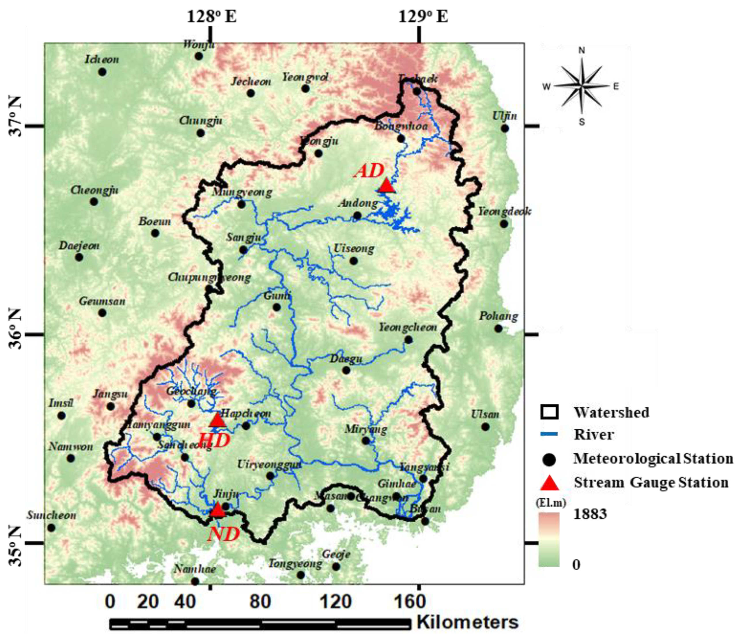
2.2.1. Study Area

As shown in Figure 1, this study selected the Nakdong River Watershed with distinct variations in spatial terrain and seasonal precipitation features as a study site. The Nakdong River Watershed is located in the south-eastern part of the Korean Peninsula, covering longitudes from 127°29′ E to 129°18′ E and latitudes from 35°03′ N to 37°13′ N. The study watershed is the second largest one (23,384 km²) in the Republic of Korea, and the main channel is the nation’s longest river (506 km) that flows from the north (Taebaek Mountains) to the south (Korean Strait). In the Nakdong River Watershed affected by the East Asian monsoon climate, the summer monsoon rainfall is concentrated from June to September. According to the past meteorological data from 2000 to 2019, the study watershed has an average annual rainfall of 1300.1 mm and an average summer rainfall of 833.9 mm [39]. For the calibration and validation of long-term daily streamflow simulations against observations, this study selected the three hydrologic stream gauge stations located at each dam reservoir inflow site, such as Andong Dam (AD), Hapcheon Dam (HD), and Nam River Dam (ND), as denoted in Figure 1 and

Table 1. Information on the three-stream gauge stations at each dam reservoir inflow site selected in the Nakdong River Watershed under study.

Station Symbol	Station Name	Latitude (°N)	Longitude (°E)	Upstream Area 1 (km2)
AD	Andong Dam	36.72	128.84	2474
HD	Hapcheon Dam	35.53	128.03	1254
ND	Nam River Dam	35.16	128.03	3151

¹ measured on the computational map projection.

. They can provide persistent long-term observations that are not affected by either flow regulations of river facilities or estuarine environments of tidal fluctuations. The dam reservoir inflow data are openly available at the Water Resources Management Information System (WAMIS) [40] managed by the Ministry of Environment.

2.2.2. Surface Boundary Conditions

The CoLM incorporating the lateral surface and subsurface flow schemes requires the SBCs in the two categories representing the vegetation and terrain features. The realistic SBCs based on the raw data of the high quality and finer resolution were constructed for the 30-km resolution grids of the CoLM computational domain under study, as provided in Lee and Choi (2017) [22]. The vegetative SBCs consist of land cover category, albedo, fractional vegetation cover, and leaf area index. The terrain SBCs include surface elevation, soil sand/clay fraction profiles, bedrock depth, and flow direction/accumulation information.

Table 2. Information on several SBCs constructed at the 30-km grids for the three study basins, AD, HD, and ND in the Nakdong River Watershed under study.

SBCs	AD	HD	ND
Land Cover Category	Savanna, Mixed Forest	Savanna, Mixed Forest	Savanna, Mixed Forest
Albedo	0.13–0.20	0.13–0.20	0.13–0.20
Fractional Vegetation Cover (%)	100	99	100
Leaf Area Index (m2/m2)	0.5–4.6	0.7–4.1	0.6–4.3
Surface Elevation (EL.m)	284.7–887.1	379.0–573.3	130.5–726.2
Sand/Clay Fraction Profile (%)	62.3/20.6	65.0/20.0	61.3/21.0
Bedrock Depth (m)	80.0–95.8	80.0	80.0–98.2

summarizes characteristics of some SBCs at 30 km grids for the three study basins, AD, HD, and ND. More detailed information on the SBCs for the Nakdong River Watershed is available in Lee and Choi (2017) [22].

2.2.3. Meteorological Forcing Data

The long-term meteorological forcing data set from 1990–2019 is based on meteorological observations from the Automated Synoptic Observing System (ASOS) in the 43 meteorological stations (see Figure 1) managed by the Korea Meteorological Administration (KMA) [39]. The meteorological forcing data to drive the CoLM standalone simulations comprises precipitation (mm), snow (cm), air pressure (hPa), temperature (°C), specific humidity (%), zonal/meridional wind speeds (m/s), and downward long/short wave radiation (MJ/m²). The meteorological point data were spatially interpolated by the Inverse Distance Weight (IDW) method and then constructed onto the 30 km computational grids for the study domain covering the Nakdong River Watershed. These construction processes are automated by the scripts in the Python programming language code developed in this study.

2.2.4. Initialization

The CoLM simulations were designed for the past 30 years from 1990–2019 in the computational study domain including the Nakdong River Watershed. The simulations from 1990–1999 were excluded to prevent any effect of the initial conditions for the state variables on simulation outcomes, and then the former ten-year simulation results from 2000–2009 and the latter ten-year simulation results from 2010–2019 were used respectively for the calibration and validation of the daily streamflow times series in the three study basins, AD, HD, and ND of the Nakdong River Watershed.

2.3. Model Calibration Approach

The calibration scheme of hydrologic models usually selects the optimal parameter set that can produce the best goodness of fit between observed data and simulated results by the model calibration criteria of the performance objective function. As for the objective function used in the hydrologic model calibration, it is desirable to include multiple metrics that can measure different aspects of model performance [41,42,43,44] and to use an appropriate objective function that can fit the performance of the model outcomes to be calibrated. Therefore, this study conducted a comparative analysis on the calibration outcomes of daily streamflow simulations from the CoLM to evaluate the model performance with respect to the strategies and characteristics of different objective functions.

One of the most popular objective functions for the performance evaluation of hydrological modelling is the NSE, as presented by Nash and Sutcliffe (1970) [29]:

$$\mathrm{NSE}=1-\frac{\sum {\left(O_i-S_i\right)}^2}{\sum {\left(O_i-\overline{O}\right)}^2}$$

(1)

where $O_i$ and $S_i$ are the observation and simulation values at a time $i$ respectively, and $\overline{O}$ is the average value of the $O_i$.

The previous studies mathematically decomposed the NSE into individual constituent components to understand relations and interactions between different metrics interrelated in the NSE [30,31,32] as

$$\mathrm{NSE}=2\mathit{\alpha }r-{\mathit{\alpha }}^2-{\mathit{\beta }}_n{}^2$$

(2)

where $r$ is the linear correlation coefficient between $S_i$ and $O_i$, $\mathit{\alpha }={\mathit{\sigma }}_s/{\mathit{\sigma }}_o$ is the relative variability measured by the standard deviation values ${\mathit{\sigma }}_s$ of $S_i$ and ${\mathit{\sigma }}_o$ of $O_i$, and ${\mathit{\beta }}_n=\left({\mathit{\mu }}_s-{\mathit{\mu }}_o\right)/{\mathit{\sigma }}_o$ is the bias where the difference between mean values ${\mathit{\mu }}_s$ of $S_i$ and ${\mathit{\mu }}_o$ of $O_i$ are normalized by the standard deviation value ${\mathit{\sigma }}_o$ of $O_i$.

Gupta et al. (2009) addressed that the bias normalized by the standard deviation of the observations in the NSE will reduce the relative importance of the bias term when the variability is high in the observations. Gupta et al. (2009) also demonstrated that the calibration result by maximizing the NSE tends to select an underestimation of the variability in the simulations. It is due to the fact that the maximum NSE is likely to be achieved when the variability ratio $\mathit{\alpha }$ is theoretically equal to the correlation coefficient $r$ always smaller than its ideal value of unity. Thus, Gupta et al. (2009) proposed a new objective function, the KGE that aggregates the three components (variability, mean, and correlation of flows) decomposed and modified from the NSE by the Euclidian distance from the ideal point in the 3-D Pareto front of the constituent components as

$$\mathrm{KGE}=1-\sqrt{{\left(\mathit{\alpha }-1\right)}^2+{\left(\mathit{\beta }-1\right)}^2+{\left(r-1\right)}^2}$$

(3)

where $\mathit{\beta }={\mathit{\mu }}_s/{\mathit{\mu }}_o$ is the ratio of the means between the simulated and observed data.

Although the KGE improves the variability in calibration results to some extent, compared with the use of NSE [32], the KGE still has a statistical tendency to underestimate the variability in the optimal simulation flows [32,34]. The KGE formulation is implicitly based on the equal weight for the three squared error metrics in Equation (3), which will be indeed equivalent to have larger weights to metric terms with larger error values, and that is the correlation error term in general or at least for our experiments. For a more balanced optimal performance on trade-offs among the three metric components in the KGE, this study has proposed the aKGE by replacing the correlation component with the adjusted correlation term normalized by the maximum correlation score (to be capable to reach its ideal value) as

$$\mathrm{aKGE}=1-\sqrt{{\left(\mathit{\alpha }-1\right)}^2+{\left(\mathit{\beta }-1\right)}^2+{\left(r_a-1\right)}^2}$$

(4)

where $r_a=r/r_{max}$ is a normalized correlation component by the maximum value $r_{max}$ of $r$ in an ensemble of simulation experiments.

3. Results and Discussion

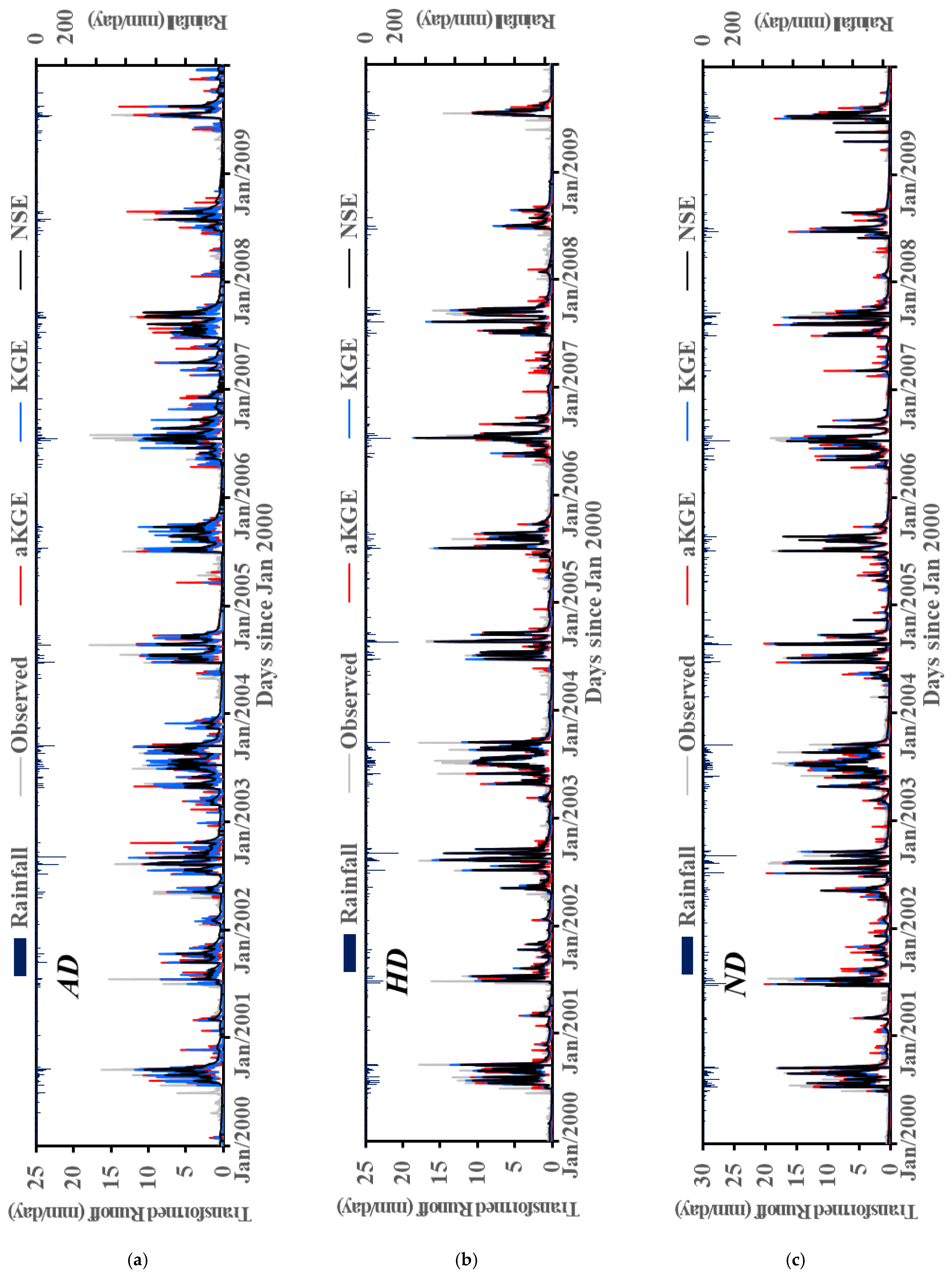
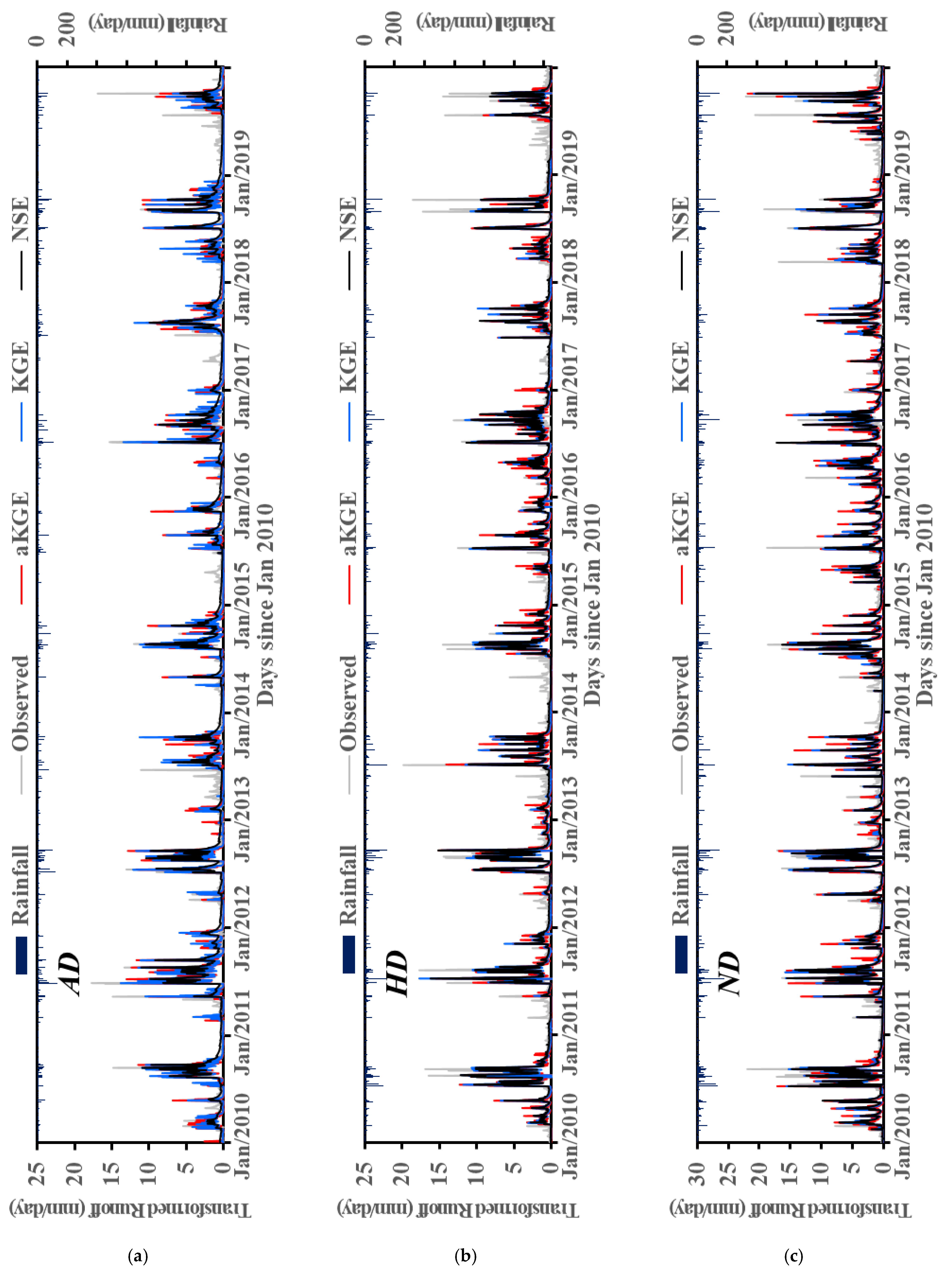
3.1. Calibration and Validation

The calibration against the daily streamflow time series from the CoLM was carried out for the model parameter set, the decay factor ƒ and the anisotropic ratio ζ of the hydraulic conductivity, as used in the previous studies [21,22,27,45,46]. An ensemble of CoLM streamflow simulations was first generated for the calibration period from 2000–2009 by a change in values of the calibration parameter sets within the feasible ranges from 2 to 9 for the decay factor ƒ and from 10 to 100,000 for the anisotropic ratio ζ. The optimal model parameters were selected by maximizing each of the three objective functions, NSE, KGE, and aKGE. The optimal parameter set achieved by each objective function was then used to simulate daily streamflow time series for the validation period from 2010–2019. Since there are differences between the real basin area and the model grid area in the three study basins, the observed and simulated streamflow values were compared by using a basin-specific runoff (streamflow per unit basin area). The daily streamflow observations from 2000–2019 were also obtained directly from the WAMIS website [40] for the three study basins, AD, HD, and ND in the Nakdong River Watershed.

Table 3. Comparison of the optimal model parameter sets and the absolute differences from unity for the three metric components, $\left|\mathit{\alpha }-1\right|$, $\left|\mathit{\beta }-1\right|$, and $\left|r-1\right|$ by each objective function, NSE, KGE, and aKGE for daily streamflow simulated from the CoLM in calibration (2000–2009) and validation (2010–2019) periods for the three study basins, AD, HD, and ND.

Station	Objective Function	Optimal Parameter		Calibration Period			Validation Period
		ƒ	ζ	$\left|\mathit{\alpha }-1\right|$	$\left|\mathit{\beta }-1\right|$	$\left|\mathit{r}-1\right|$	$\left|\mathit{\alpha }-1\right|$	$\left|\mathit{\beta }-1\right|$	$\left|\mathit{r}-1\right|$
AD	NSE	4	40,000	0.194	0.214	0.225	0.201	0.137	0.329
	KGE	8	8000	0.015	0.147	0.260	0.091	0.095	0.315
	aKGE	9	7000	0.013	0.127	0.283	0.087	0.062	0.309
HD	NSE	5	20,000	0.032	0.073	0.196	0.067	0.033	0.249
	KGE	6	20,000	0.022	0.062	0.200	0.011	0.012	0.251
	aKGE	7	6000	0.003	0.041	0.215	0.006	0.010	0.258
ND	NSE	6	90,000	0.115	0.084	0.132	0.131	0.096	0.193
	KGE	6	30,000	0.059	0.047	0.161	0.066	0.056	0.228
	aKGE	7	6000	0.016	0.000	0.189	0.015	0.013	0.262

summarizes the model calibration results to compare the absolute differences from unity for the three metric components, $\left|\mathit{\alpha }-1\right|$, $\left|\mathit{\beta }-1\right|$, and $\left|r-1\right|$ corresponding to the optimal parameter sets achieved by each objective function, NSE, KGE, and aKGE in the calibration (2000–2009) and validation (2010–2019) periods, respectively. The aKGE optimal parameter values of the decay factor ƒ and the anisotropic ratio ζ indicate a relatively smaller change over the three study basins than those by the KGE and NSE optimizations. It means the aKGE calibration can be more feasible for the model parameter regionalization in the Nakdong River Watershed. As demonstrated in Gupta et al. (2009) [32], the KGE optimal parameter sets for the three study basins can produce fewer errors in the variability α and the bias $\mathit{\beta }$ components than in the NSE optimization. In the optimization with the aKGE where the relative contribution of the correlation $r$ can become smaller by the normalization than the KGE, the error values in the variability α and the bias $\mathit{\beta }$ tend to be much lower while the correlation $r$ errors somewhat increase, compared with the both KGE and NSE calibrations in the three study basins. In particular, the aKGE improved the performance of all the three components α, $\mathit{\beta }$, and $r$ for the validation period (2010–2019) at the AD basin.

Figure 2 compares the optimal values of the three metric components, the variability $\mathit{\alpha }$, the bias $\mathit{\beta }$, and the correlation $r$ obtained by each objective function, the NSE, KGE, and aKGE over the three study basins, AD, HD, and ND in the calibration (2000–2009) and validation (2010–2019) periods, respectively. Figure 2 demonstrated that during both calibration and validation periods, the variability $\mathit{\alpha }$ and the bias $\mathit{\beta }$ components tend to be closer to the ideal value of unity in optimizing on the aKGE than in the KGE and NSE optimizations, while the correlation $r$ is much smaller than the ideal value of unity in all the three objective functions. Although the KGE was formulated based on an equal weighting of the three metric components, the possible optimal error value of the correlation $r$ will be much larger than those of the other two metric terms, thereby leading to the impact of the variability $\mathit{\alpha }$ and the bias $\mathit{\beta }$ being systematically limited on the KGE optimization outcomes. Meanwhile, the aKGE proposed for more balanced trade-offs among the three metric components in the KGE can substantially improve both variability $\mathit{\alpha }$ and bias $\mathit{\beta }$ along with a slightly inferior correlation $r$, compared with the KGE and NSE optimal results.

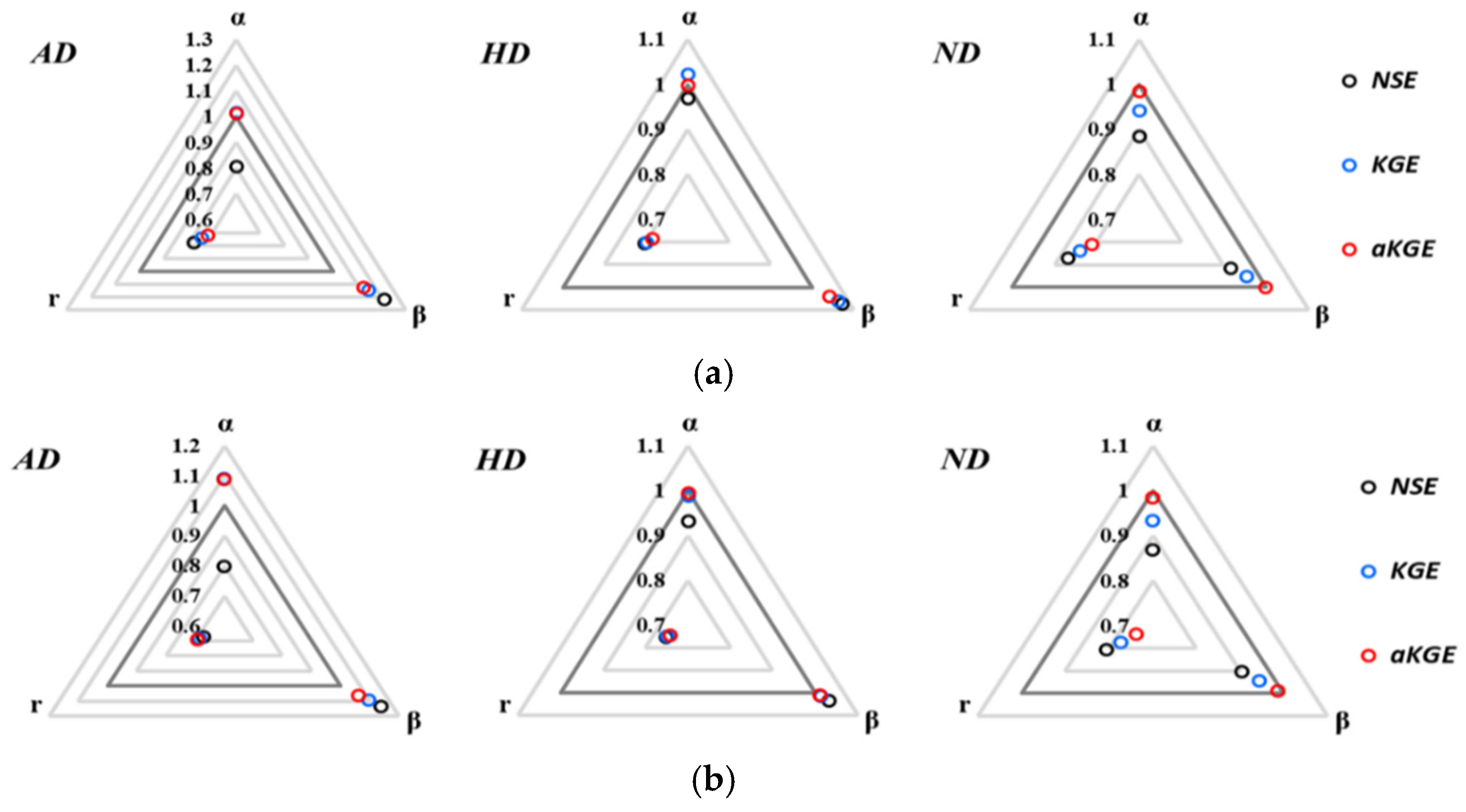
3.2. Evaluation of Streamflow Performance by Objective Functions

For the performance evaluation of daily streamflow time series, the CoLM runoff results optimized by the three objective functions, NSE, KGE, and aKGE were compared with the observed data at the three study basins, AD, HD, and ND. In the graphical comparison of the simulated and observed hydrographs, the original hydrograph is difficult to visually indicate the behavior of long-term streamflow time series for the calibration (2000–2009) and validation (2010–2019) periods. For better visualization of variations and fluctuations in daily streamflow time series, this study employed the transformed hydrograph by a power transformation method [47] as

$$Q^T=\frac{{\left(Q+1\right)}^{\mathit{\lambda }}-1}{\mathit{\lambda }}$$

(5)

where $Q^T$ is the transformed basin-specific runoff, $Q$ is the original basin-specific runoff, and $\mathit{\lambda }$ is the transformation parameter selected as 0.6 for this study.

The transformed daily time series of each basin-specific streamflow by Equation (5) were graphically compared between the optimal simulation result from the CoLM on each objective function (NSE, KGE, and aKGE) and the observed data obtained from the WAMIS in Figure 3 for the calibration period (2000–2009) and in Figure 4 for the validation period (2010–2019), respectively. Overall, in the simulation performance achieved by all the three objective functions, the long-term simulation results from the CoLM can adequately capture the interannual and seasonal variability in observed daily streamflow time series over both calibration and validation periods at the three study basins.

In the aKGE optimization with a better variability performance than the KGE and NSE, the optimal model parameter set has a clear tendency to increase the decay factor ƒ and decrease the anisotropic ratio ζ to facilitate surface flow response to rainfall, as denoted in Table 3. On the contrary, the selection of a smaller decay factor ƒ and a larger anisotropic ratio ζ will enhance subsurface runoff including baseflow, leading to lower peaks and thicker recession curves in the streamflow generation. Consequently, the aKGE optimization can substantially improve the model performance in high flow estimates compared with the optimization results by the KGE and NSE, as shown in Figure 3 and Figure 4. However, some peak flow events were not reproduced by all the three objective functions used in this study. In addition, it is implied that the improved high flow performance in the aKGE calibration can affect a better bias performance, leading to fewer water balance errors in the aKGE optimal result as well.

To statistically evaluate the model performance of the peak flow and very low flow regimes in long-term simulation results optimized by each objective function (NSE, KGE, and aKGE), the difference between observed and simulated flows was measured by the root mean square error (RMSE) as

$$\mathrm{RMSE}=\sqrt{\frac{\sum {\left(O_i-S_i\right)}^2}{n}}$$

(6)

where $n$ is the number of extreme high flows or extreme low flows belonging to the flow regime from 0 to 5% or 95 to 100%, respectively of the flow duration curve [48].

Table 4. Comparison of the root mean square error (RMSE) for extreme high flows and extreme low flows between observations and simulations optimized by each objective function, NSE, KGE, and aKGE for the calibration (2000–2009) and validation (2010–2019) periods.

Station	Objective Function	RMSE of Extreme High Flows		RMSE of Extreme Low Flows
		Calibration	Validation	Calibration	Validation
AD	NSE	0.863	0.788	0.036	0.035
	KGE	0.741	0.737	0.030	0.017
	aKGE	0.738	0.724	0.059	0.035
HD	NSE	0.962	0.871	0.014	0.039
	KGE	0.931	0.869	0.009	0.034
	aKGE	0.908	0.864	0.011	0.035
ND	NSE	1.152	1.091	0.010	0.031
	KGE	1.146	1.085	0.008	0.030
	aKGE	1.136	1.079	0.012	0.031

summarizes the RMSE values for extreme high flows and extreme low flows between the observed and simulated long-term daily streamflow time series over each ten-year period for the calibration (2000–2009) and validation (2010–2019) periods, respectively. In all the three study basins, the RMSE values for extreme high flows are lower in the optimization results by the aKGE than in those by the KGE and NSE. This is because the aKGE optimization tends to provide an improved measure of the variability performance in streamflow simulations compared with the KGE and NSE optimal results, as shown in Table 3 and Figure 2. Meanwhile, the RMSE results for extreme low flows obtained by the aKGE were not better (higher or comparable) than the KGE and NSE results. The improved variability performance is more likely to focus on the high flow regime rather than the low flow regime because the variability metric is subject to much larger errors of high flows in all the three objective functions (NSE, KGE, and aKGE) based on the mean square error. The aKGE can improve the predictability of high flows by increasing the relative contribution of the variability component to the overall model performance in the multiple criteria objective function based on the trade-offs among the different metric components.

While such a better performance of the peak flows obtained by the aKGE optimization was also found in the daily streamflow time series in Figure 3 and Figure 4, the water balance performance is difficult to be interpreted directly from the graphical comparison of daily streamflow hydrographs. For the comparative analysis of the bias performance by the choice of the three objective functions (NSE, KGE, and aKGE), Figure 5 depicts the trends and boxplots for the annual average of daily streamflow observations and simulations over the whole simulation period for the calibration (2000–2009) and the validation (2010–2019). In a boxplot graph, the box width represents the interquartile range between the first and third quartiles, and the whiskers extend to the maximum and minimum values. Overall, the annual average streamflow data obtained by the aKGE optimization showed better agreements with the observation data than those optimized by the KGE and NSE over both calibration and validation periods at the three study basins. In the boxplots for the statistical distribution of annual average streamflow data over the total simulation period of the two decades (2000–2019), it was also found that the optimal simulation results by the aKGE are more closely distributed to observations than those by the KGE and NSE at all the three study basins. This is due to the fact that the bias performance tends to be improved by an increased relative contribution of the bias measure to the overall model performance (due to a decreased relative contribution of the normalized correlation metric) when using the aKGE instead of the KGE and NSE for the model calibration.

4. Summary and Conclusions

Long-term streamflow simulations are essential to cope with water-related hazards and extreme events like severe floods and droughts caused by climate change. The Land Surface Models (LSMs) can be a useful and effective tool to simulate streamflow variations influenced by both meteorological and topographical features. The LSMs incorporating complex terrestrial hydrologic schemes generally require the model calibration process for local and empirical parameters in the streamflow generation as well. It is therefore important to use the appropriate objective function that can properly measure the model performance for the purposes of model applications (e.g., analysis of long-term water balance and streamflow extremes). The Kling and Gupta Efficiency (KGE) was presented for the balanced aggregation of equally-weighted three performance metrics consisting of variability, bias, and correlation of flows, decomposed from the Nash and Sutcliffe Efficiency (NSE) where the three components are mathematically interrelated. However, indeed, the KGE optimization is still more influenced by the correlation component that is inaccessible to the ideal value, unlike the bias and variability measures that are close to their ideal values in general. There is an obvious tendency for substantial errors in flow variability and/or average flow of streamflow simulations optimized by the use of the KGE and NSE. As a result, the calibration process with the KGE and NSE is likely to be problematic for peak flow and/or water balance analysis in long-term daily streamflow simulations. For a more balanced calibration approach in the multiple-criteria framework of the KGE, this study has therefore proposed the aKGE to improve the variability and/or bias measures through substituting an adjusted correlation term normalized by the maximum correlation score in the KGE.

To examine and evaluate the characteristics of the aKGE that differs from the KGE and NSE, the popular objective functions used in the model calibration, this study compared the performance of long-term daily streamflow simulations from an LSM, the Common Land Model (CoLM), corresponding to the calibration parameters obtained by the three objective functions, NSE, KGE, and aKGE. For the model grid-based streamflow generation in an LSM, this study selected the latest version of the CoLM incorporating the lateral flow scheme with a diffusion wave surface flow and a topographically controlled baseflow model. This version of the CoLM has been already tested for a short-term streamflow simulation over one year to evaluate the seasonal predictability at a 30-km mesoscale. This study implemented long-term streamflow simulations from the CoLM on the 30-km grids for the three study basins with the natural unregulated flows at each dam reservoir inflow site, Andong Dam (AD), Hapcheon Dam (HD), and Nam River Dam (ND) of the Nakdong River Watershed in the Republic of Korea. The long-term meteorological forcing data to drive the CoLM standalone simulations were also constructed from the point data of the 43 meteorological stations for the 30-km resolution computational domain fully covering the three study basins. This study developed a construction process for the long-term model forcing data set that can be widely used for other distributed hydrologic model studies as well.

In this study, the CoLM calibration was targeted for the decay factor ƒ and the anisotropic ratio ζ of the hydraulic conductivity, known as the most influential parameters for the streamflow generation in the CoLM. By the choice of the three objective functions, NSE, KGE, and aKGE for the model calibration against streamflow observations at the three study basins, an optimal set of the two parameters were obtained from ensemble simulations of daily streamflow time series for the calibration period from 2000 to 2009 and then evaluated for the validation period from 2010 to 2019. Compared with the model performance achieved by the KGE and NSE, the use of aKGE for the CoLM calibration systematically improved both variability and bias measures with a slightly decreased correlation score in this case study. The improved variability measure in the aKGE optimization case resulted in a better agreement between simulations and observations in the extreme high flow regime of the flow duration curve from each ten-year daily streamflow data for the calibration (2000–2009) and validation (2010–2019) periods. The general tendency to decrease the bias error in the aKGE calibration also provided a better variation and distribution of annual average streamflow that is much closer to the observation data. Such improvements to the model performance achieved by the aKGE were consistently found in all three study basins for both calibration (2000–2009) and validation (2010–2019) periods. This case study attempted to identify the optimal parameters for long-term daily streamflow time series over a sufficient simulation period of ten years each for both calibration and validation. However, the optimization outcomes in this study have not taken into account either the sensitivity of the simulation data lengths or the uncertainty in optimal parameter values to the model performance.

This study has proposed the aKGE that allows the balanced trade-offs among multiple performance measures and demonstrated the performance improvement gained by the aKGE in streamflow simulations from the CoLM at large-scale river basins targeted for mesoscale climate applications. The observed interannual and seasonal variations were successively reproduced in long-term daily streamflow simulations at the 30-km resolution from the CoLM incorporating the surface and subsurface lateral flow scheme in a grid-based LSM. Improvements to the LSM streamflow prediction will help understand the climate change impact on not only the terrestrial hydrologic cycle but also the terrestrial biodiversity and ecosystems. It is therefore expected that the streamflow modeling capability of the CoLM by an appropriate calibration approach proposed in this study can provide the basic and crucial information on the water resource management and water-related hazard assessment to cope with climate change.

In future studies, the optimal parameter regionalization can be conducted by multi-site calibration techniques because there are relatively small changes in the values of the optimal parameters on the aKGE over the three study basins. Furthermore, to improve the applicability of the CoLM to the streamflow prediction, more sensitivity analysis is required for other parameters related to terrestrial hydrologic schemes as well as resolutions in both hydrograph time series and computational grid spacing. Our modeling experiments in the present case study can, to some extent, support the fact that the aKGE will mitigate diagnostic errors in the peak flow and/or water balance of streamflow simulations rather than the KGE and NSE. However, all the three objective functions, aKGE, KGE, and NSE are not the best suited for capturing the low flow behavior because such objective functions based on the mean square error are more likely to be influenced by larger errors typically experienced in the high flow regime. It is therefore required in further research to present more feasible objective functions associate with the multiple flow regime metrics for providing the improved performance of low flows as well, which is also important for environmental and sustainable water management purposes.

References

1. Zhang, Y.; Shao, Q.; Zhang, S.; Zhai, X.; She, D. Multi-metric calibration of hydrological model to capture overall flow regimes. J. Hydrol. 2016, 539, 525–538. [Google Scholar] [CrossRef]
2. Panagoulia, D. Artificial neural networks and high and low flows in various climate regimes. Hydrol. Sci. J. 2006, 51, 563–587. [Google Scholar] [CrossRef]
3. Panagoulia, D.; Dimou, G. Sensitivity of flood events to global climate change. J. Hydrol. 1997, 191, 208–222. [Google Scholar] [CrossRef]
4. Perera, D.; Smakhtin, V.U.; Pischke, F.; Ohara, M.; Findikakis, A.; Werner, M.; Amarnath, G.; Koeppel, S.; Plotnykova, H.; Hulsmann, S. Water-related extremes and risk management. In UNESCO World Water Assessment Programme (WWAP); UN-Water. The United Nations World Water Development Report 2020: Water and Climate Change; UNSECO: Paris, France, 2020; pp. 58–67. [Google Scholar]
5. Global Runoff Data Centre. Available online: https://www.bafg.de/ (accessed on 1 May 2021).
6. Sivapalan, M.; Yaeger, M.A.; Harman, C.J.; Xu, X.; Troch, P.A. Functional model of water balance variability at the catchment scale: 1. Evidence of hydrologic similarity and space-time symmetry. Water Resour. Res. 2011, 47, W02522. [Google Scholar] [CrossRef]
7. Zaman, M.A.; Rahman, A.; Haddad, K. Regional flood frequency analysis in arid regions: A case study for Australia. J. Hydrol. 2012, 475, 74–83. [Google Scholar] [CrossRef]
8. Schaller, N.; Sillmann, J.; Müller, M.; Haarsma, R.; Hazeleger, W.; Hegdahl, T.J.; Kelder, T.; van den Oord, G.; Weerts, A.; Whan, K. The role of spatial and temporal model resolution in a flood event storyline approach in western Norway. Weather Clim. Extrem. 2020, 29, 100259. [Google Scholar] [CrossRef]
9. Lobligeois, F.; Andréassian, V.; Perrin, C.; Tabary, P.; Loumagne, C. When does higher spatial resolution rainfall information improve streamflow simulation? An evaluation using 3620 flood events. Hydrol. Earth Syst. Sci. 2014, 18, 575–594. [Google Scholar] [CrossRef] [Green Version]
10. Fisher, R.A.; Koven, C.D. Perspectives on the Future of Land Surface Models and the Challenges of Representing Complex Terrestrial Systems. J. Adv. Model. Earth Syst. 2020, 12, e2018MS001453. [Google Scholar] [CrossRef] [Green Version]
11. Blyth, E.M.; Arora, V.K.; Clark, D.B.; Dadson, S.J.; De Kauwe, M.G.; Lawrence, D.M.; Melton, J.R.; Pongratz, J.; Turton, R.H.; Yoshimura, K.; et al. Advances in Land Surface Modelling. Curr. Clim. Change Rep. 2021, 7, 45–71. [Google Scholar] [CrossRef]
12. Muleta, M.K.; Nicklow, J.W. Sensitivity and uncertainty analysis coupled with automatic calibration for a distributed watershed model. J. Hydrol. 2005, 306, 127–145. [Google Scholar] [CrossRef] [Green Version]
13. Troy, T.J.; Wood, E.F.; Sheffield, J. An efficient calibration method for continental-scale land surface modeling. Water Resour. Res. 2008, 44. [Google Scholar] [CrossRef]
14. Abbaspour, K.C.; Rouholahnejad, E.; Vaghefi, S.; Srinivasan, R.; Yang, H.; Kløve, B. A continental-scale hydrology and water quality model for Europe: Calibration and uncertainty of a high-resolution large-scale SWAT model. J. Hydrol. 2015, 524, 733–752. [Google Scholar] [CrossRef] [Green Version]
15. Parker, S.R.; Adams, S.K.; Lammers, R.W.; Stein, E.D.; Bledsoe, B.P. Targeted hydrologic model calibration to improve prediction of ecologically-relevant flow metrics. J. Hydrol. 2019, 573, 546–556. [Google Scholar] [CrossRef]
16. Bates, B.C.; Kundzewicz, Z.W.; Wu, S.; Palutikof, J.P. Climate Change and Water; Technical Paper of Intergovernmental Panel on Climate Change; IPCC Secretariat: Geneva, Switzerland, 2008; p. 210. [Google Scholar]
17. IPCC. Climate Change 2013: The Physical Science Basis. Summary for Policymakers. In Working Group I Contribution to the IPCC Fifth Assessment Report; Cambridge University Press: Cambridge, UK, 2013. [Google Scholar]
18. Sulis, M.; Paniconi, C.; Rivard, C.; Harvey, R.; Chaumont, D. Assessment of climate change impacts at the catchment scale with a detailed hydrological model of surface-subsurface interactions and comparison with a land surface model. Water Resour. Res. 2011, 47. [Google Scholar] [CrossRef]
19. Niu, G.Y.; Paniconi, C.; Troch, P.A.; Scott, R.L.; Durcik, M.; Zeng, X.; Huxman, T.; Goodrich, D.C. An integrated modelling framework of catchment-scale ecohydrological processes: 1. Model description and tests over an energy-limited watershed. Ecohydrology 2014, 7, 427–439. [Google Scholar] [CrossRef]
20. Bai, P.; Liu, X.; Yang, T.; Liang, K.; Liu, C. Evaluation of streamflow simulation results of land surface models in GLDAS on the Tibetan plateau. J. Geophys. Res. Atmos. 2016, 121, 12180–112197. [Google Scholar] [CrossRef]
21. Choi, H.I.; Liang, X.-Z.; Kumar, P. A conjunctive surface–subsurface flow representation for mesoscale land surface models. J. Hydrometeorol. 2013, 14, 1421–1442. [Google Scholar] [CrossRef]
22. Lee, J.S.; Choi, H.I. Improvements to Runoff Predictions from a Land Surface Model with a Lateral Flow Scheme Using Remote Sensing and In Situ Observations. Water 2017, 9, 148. [Google Scholar] [CrossRef] [Green Version]
23. Lin, P.; Yang, Z.-L.; Gochis, D.J.; Yu, W.; Maidment, D.R.; Somos-Valenzuela, M.A.; David, C.H. Implementation of a vector-based river network routing scheme in the community WRF-Hydro modeling framework for flood discharge simulation. Environ. Model. Softw. 2018, 107, 1–11. [Google Scholar] [CrossRef]
24. Dai, Y.; Zeng, X.; Dickinson, R.E.; Baker, I.; Bonan, G.B.; Bosilovich, M.G.; Denning, A.S.; Dirmeyer, P.A.; Houser, P.R.; Niu, G. The common land model. Bull. Am. Meteorol. Soc. 2003, 84, 1013–1024. [Google Scholar] [CrossRef] [Green Version]
25. Liang, X.-Z.; Choi, H.I.; Kunkel, K.E.; Dai, Y.; Joseph, E.; Wang, J.X.; Kumar, P. Surface boundary conditions for mesoscale regional climate models. Earth Interact. 2005, 9, 1–28. [Google Scholar] [CrossRef]
26. Choi, H.I.; Kumar, P.; Liang, X.Z. Three-dimensional volume-averaged soil moisture transport model with a scalable parameterization of subgrid topographic variability. Water Resour. Res. 2007, 43. [Google Scholar] [CrossRef] [Green Version]
27. Choi, H.I.; Liang, X.-Z. Improved terrestrial hydrologic representation in mesoscale land surface models. J. Hydrometeorol. 2010, 11, 797–809. [Google Scholar] [CrossRef]
28. Kim, E.S.; Choi, H.I.; Kim, S. Implementation of a topographically controlled runoff scheme for land surface parameterizations in regional climate models. KSCE J. Civ. Eng. 2011, 15, 1309. [Google Scholar] [CrossRef]
29. Nash, J.E.; Sutcliffe, J.V. River flow forecasting through conceptual models part I—A discussion of principles. J. Hydrol. 1970, 10, 282–290. [Google Scholar] [CrossRef]
30. Murphy, A.H. Skill scores based on the mean square error and their relationships to the correlation coefficient. Mon. Weather Rev. 1988, 116, 2417–2424. [Google Scholar] [CrossRef]
31. Wȩglarczyk, S. The interdependence and applicability of some statistical quality measures for hydrological models. J. Hydrol. 1998, 206, 98–103. [Google Scholar] [CrossRef]
32. Gupta, H.V.; Kling, H.; Yilmaz, K.K.; Martinez, G.F. Decomposition of the mean squared error and NSE performance criteria: Implications for improving hydrological modelling. J. Hydrol. 2009, 377, 80–91. [Google Scholar] [CrossRef] [Green Version]
33. Santos, L.; Thirel, G.; Perrin, C. Pitfalls in using log-transformed flows within the KGE criterion. Hydrol. Earth Syst. Sci. 2018, 22, 4583–4591. [Google Scholar] [CrossRef] [Green Version]
34. Mizukami, N.; Rakovec, O.; Newman, A.J.; Clark, M.P.; Wood, A.W.; Gupta, H.V.; Kumar, R. On the choice of calibration metrics for “high-flow” estimation using hydrologic models. Hydrol. Earth Syst. Sci. 2019, 23, 2601–2614. [Google Scholar] [CrossRef] [Green Version]
35. Kling, H.; Fuchs, M.; Paulin, M. Runoff conditions in the upper Danube basin under an ensemble of climate change scenarios. J. Hydrol. 2012, 424, 264–277. [Google Scholar] [CrossRef]
36. Fowler, K.; Peel, M.; Western, A.; Zhang, L. Improved rainfall-runoff calibration for drying climate: Choice of objective function. Water Resour. Res. 2018, 54, 3392–3408. [Google Scholar] [CrossRef] [Green Version]
37. Liang, X.Z.; Choi, H.I.; Kunkel, K.E.; Dai, Y.; Joseph, E.; Wang, J.X.L.; Kumar, P. Development of the Regional Climate-Weather Research and Forecasting Model (CWRF): Surface Boundary Conditions; ISWS SR 2005-01; Illinois State Water Survey: Champaign, IL, USA, 2005; p. 32. [Google Scholar]
38. Beven, K.J.; Kirkby, M.J. A physically based, variable contributing area model of basin hydrology/Un modèle à base physique de zone d’appel variable de l’hydrologie du bassin versant. Hydrol. Sci. J. 1979, 24, 43–69. [Google Scholar] [CrossRef] [Green Version]
39. Korea Meteorological Administration. Available online: http://www.kma.go.kr (accessed on 1 May 2021).
40. Water Management Information System. Available online: http://www.wamis.go.kr/wkd/mn_dammain.aspx (accessed on 1 May 2021).
41. Bastidas, L.; Gupta, H.V.; Sorooshian, S.; Shuttleworth, W.J.; Yang, Z. Sensitivity analysis of a land surface scheme using multicriteria methods. J. Geophys. Res. Atmos. 1999, 104, 19481–19490. [Google Scholar] [CrossRef] [Green Version]
42. Bastidas, L.A.; Hogue, T.; Sorooshian, S.; Gupta, H.V.; Shuttleworth, W.J. Parameter sensitivity analysis for different complexity land surface models using multicriteria methods. J. Geophys. Res. Atmos. 2006, 111. [Google Scholar] [CrossRef] [Green Version]
43. Van Werkhoven, K.; Wagener, T.; Reed, P.; Tang, Y. Sensitivity-guided reduction of parametric dimensionality for multi-objective calibration of watershed models. Adv. Water Resour. 2009, 32, 1154–1169. [Google Scholar] [CrossRef]
44. Neelin, J.D.; Bracco, A.; Luo, H.; McWilliams, J.C.; Meyerson, J.E. Considerations for parameter optimization and sensitivity in climate models. Proc. Natl. Acad. Sci. USA 2010, 107, 21349–21354. [Google Scholar] [CrossRef] [PubMed] [Green Version]
45. Chen, J.; Kumar, P. Topographic influence on the seasonal and interannual variation of water and energy balance of basins in North America. J. Clim. 2001, 14, 1989–2014. [Google Scholar] [CrossRef]
46. Kumar, P. Layer averaged Richard’s equation with lateral flow. Adv. Water Resour. 2004, 27, 521–531. [Google Scholar] [CrossRef]
47. Yilmaz, K.K.; Gupta, H.V.; Wagener, T. A process-based diagnostic approach to model evaluation: Application to the NWS distributed hydrologic model. Water Resour. Res. 2008, 44. [Google Scholar] [CrossRef] [Green Version]
48. Pfannerstill, M.; Guse, B.; Fohrer, N. Smart low flow signature metrics for an improved overall performance evaluation of hydrological models. J. Hydrol. 2014, 510, 447–458. [Google Scholar] [CrossRef]
Figure 1. The location map of the three-stream gauge stations (red triangular points) upstream of the Nakdong River (blue lines) selected in the Nakdong River Watershed (black lines) under study, along with the 43 meteorological stations (black dots) used for constructing the meteorological forcing data in the CoLM computational domain (outer frame).
Water 13 01709 g001
Figure 2. The radar chart of the optimal metric components, variability α , bias β , and correlation r obtained by each objective function, NSE, KGE, and aKGE for the three study basins, AD, HD, and ND in (a) the calibration period (2000–2009), and (b) the validation period (2010–2019).
Water 13 01709 g002
Figure 3. Comparison of daily hydrograph time series for the CoLM simulations optimized by the three objective functions, NSE, KGE, and aKGE and the observations at the three study basins: (a) AD, (b) HD, and (c) ND over the calibration period from 2000 to 2009. All hydrographs are transformed from each basin-specific streamflow data by a power transformation function in Equation (5) for better visualization of variations and fluctuations in daily streamflow time series.
Water 13 01709 g003
Figure 4. Comparison of daily hydrograph time series for the CoLM simulations optimized by the three objective functions, NSE, KGE, and aKGE and the observations at the three study basins: (a) AD, (b) HD, and (c) ND over the validation period from 2010 to 2019. All hydrographs are transformed from each basin-specific streamflow data by a power transformation function in Equation (5) for better visualization of variations and fluctuations in daily streamflow time series.
Water 13 01709 g004
Figure 5. Comparison of annual average streamflow trends for the observations and the CoLM simulations optimized by the three objective functions, NSE, KGE, and aKGE at the three study basins: (a) AD, (b) HD, and (c) ND for the total simulation period from 2000 to 2019. The boxplot for annual average streamflow represents the 25th, 50th, and 75th percentile values along with the mean value by the ‘x’ symbol, and the whisker plot extends to the maximum and minimum values from the box.
Water 13 01709 g005