
Middle Holocene Climate Oscillations Recorded in the Western Dvina Lakeland

 , , , , , ,
  , , , and
Abstract
1. Introduction
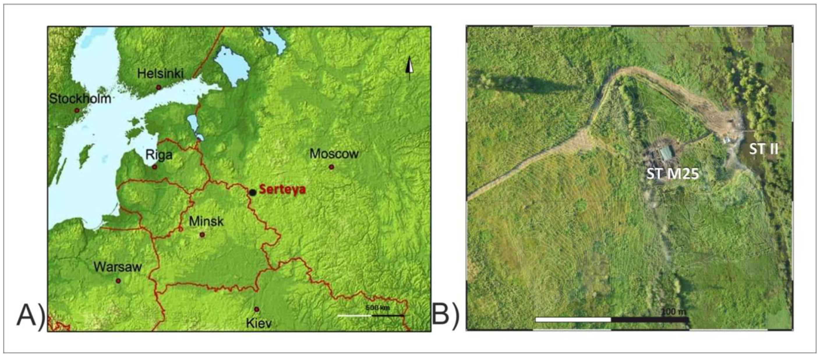
2. Study Area
Archeological Investigation
3. Materials and Methods
3.1. Field Studies and Coring
- 0–23 cm b.g.l.—20th century AD embankment
- 23–65 cm b.g.l.—peaty organic mud with sandy admixtures
- 65–75/80 cm b.g.l.—carbonate sandy organic mud
- 75/80–148.5 cm b.g.l.—coarse detritus gyttja
- 148.5–160 cm b.g.l.—sand and gravel with organic mud and plant detritus
3.2. Paleoecological Analyses
3.2.1. Chironomidae—Laboratory Techniques, Identification, and Statistics
3.2.2. Cladocera—Laboratory Techniques, Identification, and Statistics
3.2.3. Pollen—Laboratory Techniques, Identification, and Statistics
3.3. Temperature, Precipitation, and Water Depth Reconstructions
4. Results and Interpretation
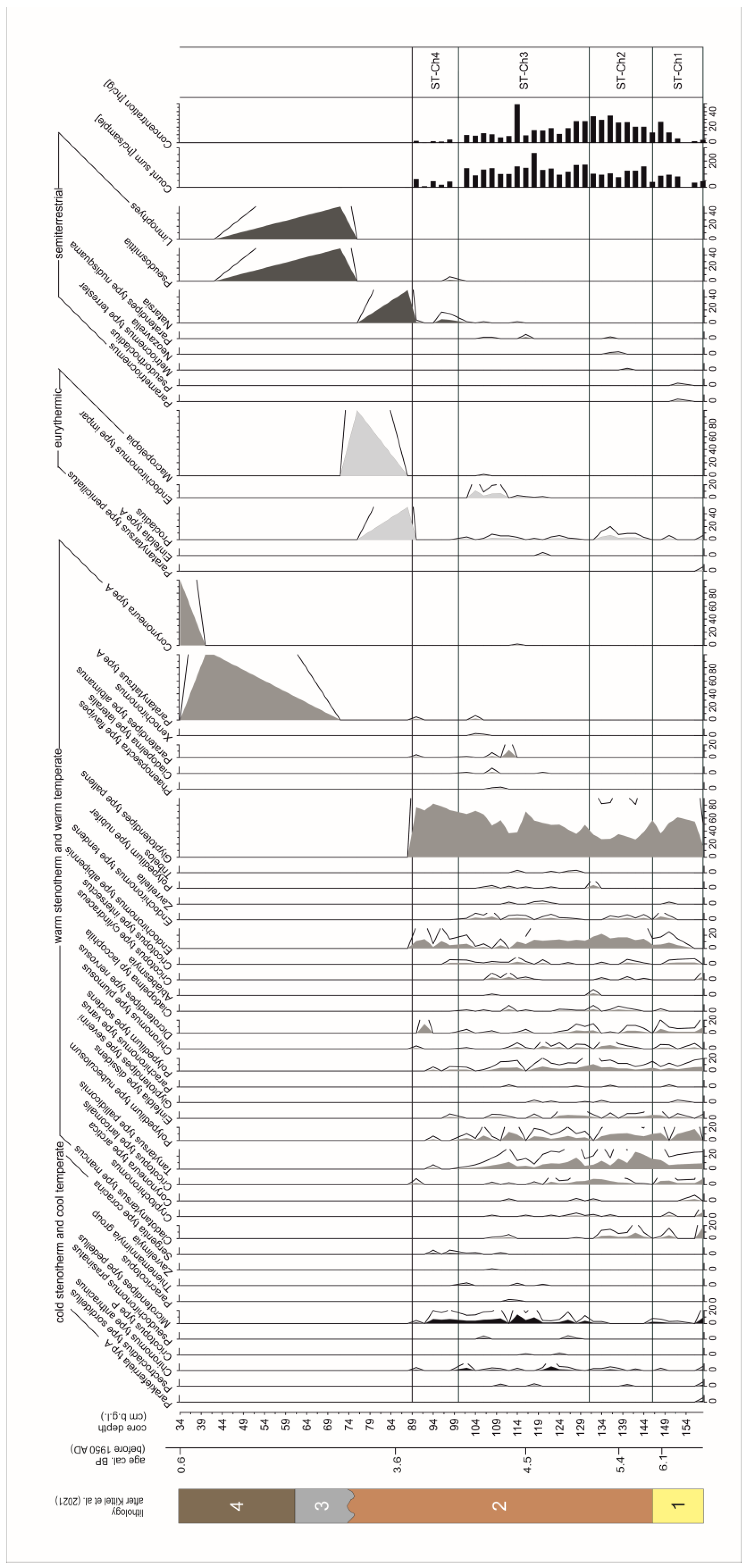
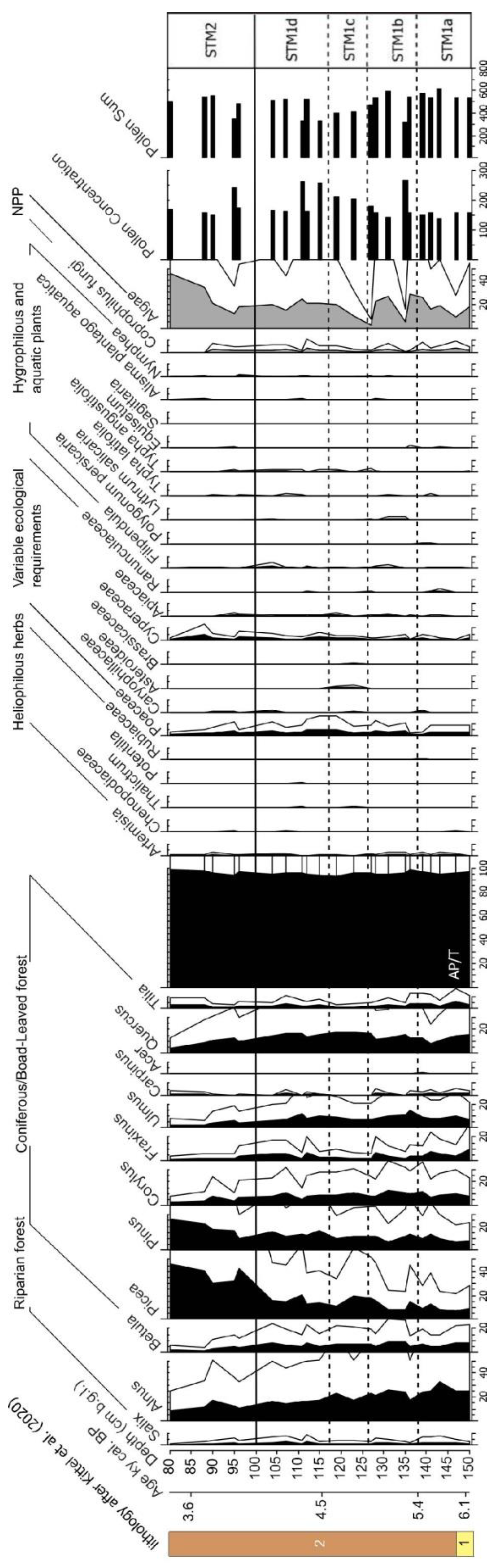
4.1. Chironomidae, Cladocera, and Pollen Assemblage Stratigraphy
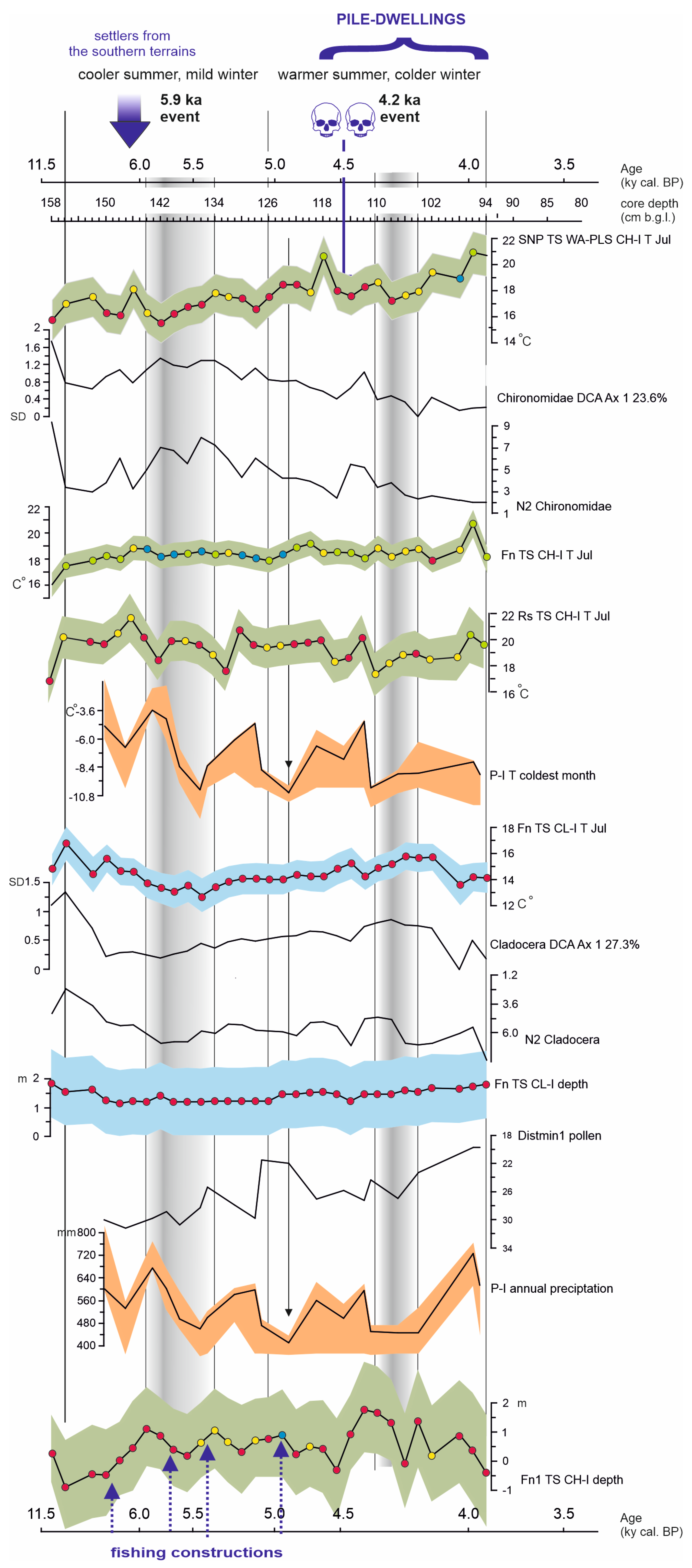
4.2. Results and Interpretation of Climatic and Hydroclimatic Reconstructions
4.2.1. Detrended Correspondence Analysis
4.2.2. The Chironomidae-Inferred and Cladocera-Inferred Mean Summer Air Temperature Reconstructions
4.2.3. The Pollen-Inferred Temperature of the Coldest Month and Annual Precipitation Reconstructions
4.2.4. The Cladocera-Inferred and Chironomidae-Inferred Lake Water Level Reconstructions
5. Discussion
6. Conclusions
Supplementary Materials
Author Contributions
Funding
Institutional Review Board Statement
Informed Consent Statement
Data Availability Statement
Conflicts of Interest
References
- Sánchez Goñi, M.F.; Ortu, E.; Banks, W.E.; Giraudeau, J.; Leroyer, C.; Hanquiez, V. The expansion of Central and Northern European Neolithic populations was associated with a multi-century warm winter and wetter climate. Holocene 2016, 26, 1188–1199. [Google Scholar] [CrossRef]
- Kulkova, M.; Mazurkevich, A.; Dolbunova, E.; Lozovsky, V. The 8200 calBP climate event and the spread of the Neolithic in Eastern Europe. Doc. Praehist. 2015, 42, 77–92. [Google Scholar] [CrossRef][Green Version]
- Warden, L.; Moros, M.; Neumann, T.; Shennan, S.; Timpson, A.; Manning, K.; Sollai, M.; Wacker, L.; Perner, K.; Häusler, K. Climate induced human demographic and cultural change in northern Europe during the mid-Holocene. Sci. Rep. 2017, 7, 15251. [Google Scholar] [CrossRef] [PubMed]
- Kaufman, D.; McKay, N.; Routson, C.; Erb, M.; Davis, B.; Heiri, O.; Jaccard, S.; Tierney, J.; Dätwyler, C.; Axford, Y. A global database of Holocene paleotemperature records. Sci. Data 2020, 7, 115. [Google Scholar] [CrossRef]
- Khomutova, V.I.; Elina, G.A. Stratigraphy of lake sediments by palynological data. Istoria Ladozhskogo, Onezhskogo, Pskovsko- Chudskogo ozer, Baikala i Khanki [The history of Ladoga, Onego, Pskovsko-Chudskoe, Baikal and Khanki lakes]. 1990. pp. 92–96.
- Elina, G.; Filimonova, L.; Raukas, A.; Saarse, L. Late-Glacial Vegetation on the Territory of Karelia. In Palaeohydrology of the Temperate Zone III: Mires and Lakes; Valgus: Tallinn, Estonia, 1987; pp. 53–69. [Google Scholar]
- Nazarova, L.; Syrykh, L.S.; Mayfield, R.J.; Frolova, L.A.; Ibragimova, A.G.; Grekov, I.M.; Subetto, D.A. Palaeoecological and palaeoclimatic conditions on the Karelian Isthmus (northwestern Russia) during the Holocene. Quat. Res. 2020, 95, 65–83. [Google Scholar] [CrossRef]
- Nazarova, L.B.; Subetto, D.A.; Syrykh, L.S.; Grekov, I.M.; Leontev, P.A. Reconstructions of Paleoecological and Paleoclimatic Conditions of the Late Pleistocene and Holocene according to the Results of Chironomid Analysis of Sediments from Medvedevskoe Lake (Karelian Isthmus). Dokl. Earth Sci. 2018, 480, 710. [Google Scholar] [CrossRef]
- Feurdean, A.; Perşoiu, A.; Tanţău, I.; Stevens, T.; Magyari, E.K.; Onac, B.P.; Marković, S.; Andrič, M.; Connor, S.; Fărcaş, S. Climate variability and associated vegetation response throughout Central and Eastern Europe (CEE) between 60 and 8 ka. Quat. Sci. Rev. 2014, 106, 206–224. [Google Scholar] [CrossRef]
- Moreno, A.; Svensson, A.; Brooks, S.J.; Connor, S.; Engels, S.; Fletcher, W.; Genty, D.; Heiri, O.; Labuhn, I.; Perşoiu, A. A compilation of Western European terrestrial records 60–8 ka BP: Towards an understanding of latitudinal climatic gradients. Quat. Sci. Rev. 2014, 106, 167–185. [Google Scholar] [CrossRef]
- Berntsson, A.; Rosqvist, G.C.; Velle, G. Late-Holocene temperature and precipitation changes in Vindelfjällen, mid-western Swedish Lapland, inferred from chironomid and geochemical data. Holocene 2014, 24, 78–92. [Google Scholar] [CrossRef]
- Heinsalu, A.; Veski, S. The history of the Yoldia Sea in Northern Estonia: Palaeoenvironmental conditions and climatic oscillations. Geol. Q. 2007, 51, 295–306. [Google Scholar]
- Kremenetski, K.; Borisova, O.; Zelikson, E. The Late Glacial and Holocene history of vegetation in the Moscow region. Paleontol. J. C/C Paleontol. Zhurnal 2000, 34, 67–74. [Google Scholar]
- Sapelko, T.V. Dinamika razvitiâ rastitel’nosti na territorii Kenozerskogo nacional’nogo parka v golocene. Izv. Rus. Geogr. Obŝestva 2006, 138, 70–76. [Google Scholar]
- Velichko, A.A.; Andreev, A.; Klimanov, V. Climate and vegetation dynamics in the tundra and forest zone during the Late Glacial and Holocene. Quat. Int. 1997, 41, 71–96. [Google Scholar] [CrossRef]
- Velichko, A.A.; Catto, N.; Drenova, A.N.; Klimanov, V.A.; Kremenetski, K.V.; Nechaev, V.P. Climate changes in East Europe and Siberia at the Late glacial–holocene transition. Quat. Int. 2002, 91, 75–99. [Google Scholar] [CrossRef]
- Kołaczek, P.; Karpińska-Kołaczek, M.; Marcisz, K.; Gałka, M.; Lamentowicz, M. Palaeohydrology and the human impact on one of the largest raised bogs complex in the Western Carpathians (Central Europe) during the last two millennia. Holocene 2018, 28, 595–608. [Google Scholar] [CrossRef]
- Brooks, S.J.; Heiri, O.; Langdon, P.G. The Identification and Use of Palaearctic Chironomidae Larvae in Palaeoecology; Quaternary Research Association: London, UK, 2007. [Google Scholar]
- Oliver, D. Life history of the Chironomidae. Annu. Rev. Entomol. 1971, 16, 211–230. [Google Scholar] [CrossRef]
- Eggermont, H.; Heiri, O. The chironomid-temperature relationship: Expression in nature and palaeoenvironmental implications. Biol. Rev. 2012, 87, 430–456. [Google Scholar] [CrossRef]
- Kotrys, B.; Płóciennik, M.; Sydor, P.; Brooks, S.J. Expanding the Swiss-Norwegian chironomid training set with Polish data. Boreas 2020, 49, 89–107. [Google Scholar] [CrossRef]
- Magny, M.; Combourieu-Nebout, N.; De Beaulieu, J.-L.; Bout-Roumazeilles, V.; Colombaroli, D.; Desprat, S.; Francke, A.; Joannin, S.; Ortu, E.; Peyron, O. North–south palaeohydrological contrasts in the central Mediterranean during the Holocene: Tentative synthesis and working hypotheses. Clim. Past 2013, 9, 2043–2071. [Google Scholar] [CrossRef]
- Frolova, L.; Nazarova, L.; Pestryakova, L.; Herzschuh, U. Analysis of the effects of climate-dependent factors on the formation of zooplankton communities that inhabit arctic lakes in the Anabar River Basin. Contemp. Probl. Ecol. 2013, 6, 1–11. [Google Scholar] [CrossRef]
- Płóciennik, M.; Pawłowski, D.; Vilizzi, L.; Antczak-Orlewska, O. From oxbow to mire: Chironomidae and Cladocera as habitat palaeoindicators. Hydrobiologia 2020, 847, 3257–3275. [Google Scholar] [CrossRef]
- Luoto, T.P.; Kivilä, E.H.; Kotrys, B.; Płóciennik, M.; Rantala, M.V.; Nevalainen, L. Air temperature and water level inferences from northeastern Lapland (69 N) since the Little Ice Age. Pol. Polar Res. 2020, 23–40. [Google Scholar] [CrossRef]
- Pawłowski, D.; Płóciennik, M.; Brooks, S.J.; Luoto, T.P.; Milecka, K.; Nevalainen, L.; Peyron, O.; Self, A.; Zieliński, T. A multiproxy study of Younger Dryas and Early Holocene climatic conditions from the Grabia River paleo-oxbow lake (central Poland). Palaeogeogr. Palaeoclimatol. Palaeoecol. 2015, 438, 34–50. [Google Scholar] [CrossRef]
- Pawłowski, D.; Kowalewski, G.; Milecka, K.; Płóciennik, M.; Woszczyk, M.; Zieliński, T.; Okupny, D.; Włodarski, W.; Forysiak, J. A reconstruction of the palaeohydrological conditions of a flood-plain: A multi-proxy study from the Grabia River valley mire, central Poland. Boreas 2015, 44, 543–562. [Google Scholar] [CrossRef]
- Nevalainen, L.; Sarmaja-Korjonen, K.; Luoto, T.P. Sedimentary Cladocera as indicators of past water-level changes in shallow northern lakes. Quat. Res. 2011, 75, 430–437. [Google Scholar] [CrossRef]
- Pawłowski, D.; Borówka, R.K.; Kowalewski, G.; Luoto, T.P.; Milecka, K.; Nevalainen, L.; Okupny, D.; Płóciennik, M.; Woszczyk, M.; Tomkowiak, J. The response of flood-plain ecosystems to the Late Glacial and Early Holocene hydrological changes: A case study from a small Central European river valley. Catena 2016, 147, 411–428. [Google Scholar] [CrossRef]
- Pawłowski, D.; Borówka, R.K.; Kowalewski, G.A.; Luoto, T.P.; Milecka, K.; Nevalainen, L.; Okupny, D.; Tomkowiak, J.; Zieliński, T. Late Weichselian and Holocene record of the paleoenvironmental changes in a small river valley in Central Poland. Quat. Sci. Rev. 2016, 135, 24–40. [Google Scholar] [CrossRef]
- Nevalainen, L.; Luoto, T.P.; Kultti, S.; Sarmaja-Korjonen, K. Do subfossil Cladocera and chydorid ephippia disentangle Holocene climate trends? Holocene 2012, 22, 291–299. [Google Scholar] [CrossRef]
- Pawłowski, D. Younger Dryas climatic reconstructions in central Poland. Acta Geol. Pol. 2017, 67, 567–584. [Google Scholar] [CrossRef][Green Version]
- Marcisz, K.; Gałka, M.; Pietrala, P.; Miotk-Szpiganowicz, G.; Obremska, M.; Tobolski, K.; Lamentowicz, M. Fire activity and hydrological dynamics in the past 5700 years reconstructed from Sphagnum peatlands along the oceanic–continental climatic gradient in northern Poland. Quat. Sci. Rev. 2017, 177, 145–157. [Google Scholar] [CrossRef]
- Gałka, M.; Miotk-Szpiganowicz, G.; Marczewska, M.; Barabach, J.; van der Knaap, W.O.; Lamentowicz, M. Palaeoenvironmental changes in Central Europe (NE Poland) during the last 6200 years reconstructed from a high-resolution multi-proxy peat archive. Holocene 2015, 25, 421–434. [Google Scholar] [CrossRef]
- Lamentowicz, M.; Lamentowicz, Ł.; van der Knaap, W.O.; Gąbka, M.; Mitchell, E.A.D. Contrasting Species—Environment Relationships in Communities of Testate Amoebae, Bryophytes and Vascular Plants Along the Fen–Bog Gradient. Microb. Ecol. 2010, 59, 499–510. [Google Scholar] [CrossRef] [PubMed]
- Heikkilae, M.E.; Seppä, H. Holocene climate dynamics in Latvia, eastern Baltic region: A pollen based summer temperature reconstruction and regional comparison. Boreas 2010, 39, 705–719. [Google Scholar] [CrossRef]
- Sohar, K.; Kalm, V. A 12.8-ka-long palaeoenvironmental record revealed by subfossil ostracod data from lacustrine freshwater tufa in Lake Sinijärv, northern Estonia. J. Paleolimnol. 2008, 40, 809–821. [Google Scholar] [CrossRef]
- Šeirienė, V.; Kabailienė, M.; Kasperovičienė, J.; Mažeika, J.; Petrošius, R.; Paškauskas, R. Reconstruction of postglacial palaeoenvironmental changes in eastern Lithuania: Evidence from lacustrine sediment data. Quat. Int. 2009, 207, 58–68. [Google Scholar] [CrossRef]
- Stivrins, N.; Kalnina, L.; Veski, S.; Zeimule, S. Local and regional Holocene vegetation dynamics at two sites in eastern Latvia. Boreal Environ. Res. 2014, 19, 310–322. [Google Scholar]
- Terasmaa, J.; Puusepp, L.; Marzecová, A.; Vandel, E.; Vaasma, T.; Koff, T. Natural and human-induced environmental changes in Eastern Europe during the Holocene: A multi-proxy palaeolimnological study of a small Latvian lake in a humid temperate zone. J. Paleolimnol. 2013, 49, 663–678. [Google Scholar] [CrossRef]
- Syrykh, L.; Subetto, D.; Nazarova, L. Paleolimnological studies on the East European Plain and nearby regions: The PaleoLake Database. J. Paleolimnol. 2021, 65, 369–375. [Google Scholar] [CrossRef]
- Subetto, D.; Nazarova, L.; Pestryakova, L.; Syrykh, L.; Andronikov, A.; Biskaborn, B.; Diekmann, B.; Kuznetsov, D.; Sapelko, T.; Grekov, I. Paleolimnological studies in Russian northern Eurasia: A review. Contemp. Probl. Ecol. 2017, 10, 327–335. [Google Scholar] [CrossRef]
- Arslanov, K.A.; Savelieva, L.; Klimanov, V.; Chernov, S.; Maksimov, F.; Tertychnaya, T.; Subetto, D. New data on chronology of landscape-paleoclimatic stages in Northwestern Russia during the Late Glacial and Holocene. Radiocarbon 2001, 43, 581–594. [Google Scholar] [CrossRef][Green Version]
- Novik, A.; Punning, J.-M.; Zernitskaya, V. The development of Belarusian lakes during the Late Glacial and Holocene. Est. J. Earth Sci. 2010, 59, 63–79. [Google Scholar] [CrossRef]
- Novenko, E.; Glasko, M.; Volkova, E.; Ziuganova, I. Dinamika landšaftov i klimata bassejna verhnego Dona v srednem i pozdnem golocene. Izvestiâ Akademii nauk SSSR. Seria geografičeskaâ 2013, 2, 68–82. [Google Scholar]
- Arslanov, K.A.; Saveljeva, L.; Gey, N.; Klimanov, V.; Chernov, S.; Chernova, G.; Kuzmin, G.; Tertychnaya, T.; Subetto, D.; Denisenkov, V. Chronology of vegetation and paleoclimatic stages of northwestern Russia during the Late Glacial and Holocene. Radiocarbon 1999, 41, 25–45. [Google Scholar] [CrossRef]
- Nazarova, L.; Herzschuh, U.; Wetterich, S.; Kumke, T.; Pestryakova, L. Chironomid-based inference models for estimating mean July air temperature and water depth from lakes in Yakutia, northeastern Russia. J. Paleolimnol. 2011, 45, 57–71. [Google Scholar] [CrossRef]
- Nazarova, T.; Fomin, I.; Dmitriev, P.; Wendt, J.; Janaleyeva, K. Landscape and limnological research of lake systems of the northeastern borderlands of the Republic of Kazakhstan and assesment of their recreational capacity. Geoj. Tour. Geosites 2019, 25, 485–495. [Google Scholar] [CrossRef]
- Druzhinina, O.; Kublitskiy, Y.; Stančikaite, M.; Nazarova, L.; Syrykh, L.; Gedminiene, L.; Uogintas, D.; Skipityte, R.; Arslanov, K.; Vaikutiene, G. The Late Pleistocene–Early Holocene palaeoenvironmental evolution in the SE Baltic region: A new approach based on chironomid, geochemical and isotopic data from Kamyshovoye Lake, Russia. Boreas 2020, 49, 544–561. [Google Scholar] [CrossRef]
- Nazarova, L.B.; Sapelko, T.V.; Kuznetsov, D.D.; Syrykh, L.S. Palaeoecological and Palaeoclimatical Reconstructions of Holocene According Chironomid Analysis of Lake Glubokoye Sediments. In Doklady Biological Sciences: Proceedings of the Academy of Sciences of the USSR, Biological Sciences Sections; Pleiades Publishing: New York, NY, USA, 2015; Volume 460, pp. 57–60. [Google Scholar] [CrossRef]
- Rinterknecht, V.; Hang, T.; Gorlach, A.; Kohv, M.; Kalla, K.; Kalm, V.; Subetto, D.; Bourlès, D.; Léanni, L.; Guillou, V. The Last Glacial Maximum extent of the Scandinavian Ice Sheet in the Valday Heights, western Russia: Evidence from cosmogenic surface exposure dating using 10Be. Quat. Sci. Rev. 2018, 200, 106–113. [Google Scholar] [CrossRef]
- Mazurkevich, A.; Dolbunova, E.; Kittel, P.; Fassbender, J.; Maigrot, Y.; Mroczkowska, A.; Płóciennik, M.; Sikora, J.; Słowiński, M.; Sablin, M. Multi-Disciplinary Research on the Neolithic Pile-Dwelling Serteya II Site (Western Russia) and the Landscape Reconstruction. Nie tylko Krzemienie. Not only flints.; Instytut Archeologii Uniwersytetu Łódzkiego, Łódzka Fundacja Badań Naukowych, Stowarzyszenie Naukowe Archeologów Polskich Oddział w Łodzi: Łódź, Poland, 2017; pp. 103–128. [Google Scholar]
- Mazurkevich, A.; Kulkova, M.; Savel’eva, L. Geoarchaeology of the Serteya Microregion, the Upper Dvina Basin. In Geoarchaeological Issues of the Upper Dnieper–Western Dvina River Region (Western Russia); Universum: Moscow-Smolensk, Russia, 2012; pp. 49–104. [Google Scholar]
- Mazurkevich, A.N.; Arslanov, K.A.; Savel’eva, L.A.; Kulkova, M.A.; Zaitseva, G.I. Mesolithic and Neolithic in the Western Dvina–Lovat Area. In The East European Plain on the Eve of Agriculture; BAR International Series; Archaeopress: Oxford, UK, 2009; Volume 164, pp. 145–153. [Google Scholar]
- Kulkova, M.; Mazurkevich, A.; Dolbunova, E.; Regert, M.; Mazuy, A.; Nesterov, E.; Sinai, M. Late Neolithic Subsistence Strategy and Reservoir Effects in 14C Dating of Artifacts at the Pile-Dwelling Site Serteya II (NW Russia). Radiocarbon 2015, 57, 611–623. [Google Scholar] [CrossRef][Green Version]
- Mazurkevich, A.N.; Korotkevich, B.N.; Dolukhanov, P.M.; Shukurov, A.M.; Arslanov, K.A.; Savel’eva, L.A.; Dzinoridze, E.N.; Kulkova, M.A.; Zaitseva, G.I. Climate, subsistence and human movements in the Western Dvina—Lovat River Basins. Quaternary International. Quat. Int. 2009, 203, 52–66. [Google Scholar] [CrossRef]
- Kittel, P.; Mazurkevich, A.; Wieckowska-Lüth, M.; Pawłowski, D.; Dolbunova, E.; Płóciennik, M.; Gauthier, E.; Krąpiec, M.; Maigrot, Y.; Danger, M. On the border between land and water: The environmental conditions of the Neolithic occupation from 4.3 until 1.6 ka BC at Serteya, Western Russia. Geoarchaeology 2021, 36, 173–202. [Google Scholar] [CrossRef]
- Kulkova, M.; Mazurkevich, A.; Dolukhanov, P. Chronology and paleoclimate of prehistoric sites in Western Dvina-Lovat area of North-western Russia. Geochronometria: J. Methods Appl. Absol. Chronol. 2001, 20, 87–94. [Google Scholar]
- Mazurkevich, A.; Dolbunova, E.; Kul’kova, M.; Alexandrovskiy, A.; Saveleva, L.; Polkovnikova, M.; Khrustaleva, I.; Kolosova, M.; Hookk, D.; Mazurkevich, K. Dynamics of landscape developing in early-middle Neolithics in Dnepr-Dvina region. In Proceedings of the International Conference “Geomorphic Processes and Geoarchaeology: From Landscape Archaeology to Archaeotourism”; Universum: Moscow-Smolensk, Russia, 2012; pp. 20–24. [Google Scholar]
- Mazurkevich, A.N.; Hookk, D.Y.; Fassbinder, J. Magnetometry and susceptibility prospecting on Neolithic-early Iron Age sites at Serteya, North-West Russia. ArcheoSciences Revue D’archeometrie 2009, 33, 81–85. [Google Scholar] [CrossRef]
- Mazurkevich, A.N. Pervyye svidetelstva proyavleniya proizvodyashchego khozyaystva na Severo-Zapade Rossii. In Pushkarevskiy sbornik II; Izd-vo S-Peterburgskogo un-ta: Sankt Petersburg, Russia, 2003; pp. 77–84. [Google Scholar]
- Tarasov, P.E.; Savelieva, L.A.; Long, T.; Leipe, C. Postglacial vegetation and climate history and traces of early human impact and agriculture in the present-day cool mixed forest zone of European Russia. Quat. Int. 2019, 516, 21–41. [Google Scholar] [CrossRef]
- Bond, G.; Kromer, B.; Beer, J.; Muscheler, R.; Evans, M.N.; Showers, W.; Hoffmann, S.; Lotti-Bond, R.; Hajdas, I.; Bonani, G. Persistent solar influence on North Atlantic climate during the Holocene. Science 2001, 294, 2130–2136. [Google Scholar] [CrossRef]
- Obrochta, S.P.; Miyahara, H.; Yokoyama, Y.; Crowley, T.J. A re-examination of evidence for the North Atlantic “1500-year cycle” at Site 609. Quat. Sci. Rev. 2012, 55, 23–33. [Google Scholar] [CrossRef]
- Bütikofer, J. Millennial Scale Climate Variability during the Last 6000 Years-Tracking down the Bond Cycles. Verlag nicht ermittelbar. 2007. [Google Scholar]
- Solanki, S.; Usoskin, I.; Kromer, B.; Schüssler, M.; Beer, J. How unusual is today’s solar activity?(reply). Nature 2005, 436, E4–E5. [Google Scholar] [CrossRef][Green Version]
- Wang, W.; Feng, Z.; Ran, M.; Zhang, C. Holocene climate and vegetation changes inferred from pollen records of Lake Aibi, northern Xinjiang, China: A potential contribution to understanding of Holocene climate pattern in East-central Asia. Quat. Int. 2013, 311, 54–62. [Google Scholar] [CrossRef]
- Mayewski, P.A.; Rohling, E.E.; Stager, J.C.; Karlén, W.; Maasch, K.A.; Meeker, L.D.; Meyerson, E.A.; Gasse, F.; van Kreveld, S.; Holmgren, K. Holocene climate variability. Quat. Res. 2004, 62, 243–255. [Google Scholar] [CrossRef]
- Newman, M.; Alexander, M.A.; Ault, T.R.; Cobb, K.M.; Deser, C.; Di Lorenzo, E.; Mantua, N.J.; Miller, A.J.; Minobe, S.; Nakamura, H. The Pacific decadal oscillation, revisited. J. Clim. 2016, 29, 4399–4427. [Google Scholar] [CrossRef]
- Trigo, R.M.; Osborn, T.J.; Corte-Real, J.M. The North Atlantic Oscillation influence on Europe: Climate impacts and associated physical mechanisms. Clim. Res. 2002, 20, 9–17. [Google Scholar] [CrossRef]
- Visbeck, M.H.; Hurrell, J.W.; Polvani, L.; Cullen, H.M. The North Atlantic Oscillation: Past, present, and future. Proc. Natl. Acad. Sci. USA 2001, 98, 12876–12877. [Google Scholar] [CrossRef]
- Cronin, T.; Hayo, K.; Thunell, R.; Dwyer, G.; Saenger, C.; Willard, D. The medieval climate anomaly and little ice age in Chesapeake Bay and the North Atlantic Ocean. Palaeogeogr. Palaeoclimatol. Palaeoecol. 2010, 297, 299–310. [Google Scholar] [CrossRef]
- Wanner, H.; Beer, J.; Bütikofer, J.; Crowley, T.J.; Cubasch, U.; Flückiger, J.; Goosse, H.; Grosjean, M.; Joos, F.; Kaplan, J.O.; et al. Mid- to Late Holocene climate change: An overview. Quat. Sci. Rev. 2008, 27, 1791–1828. [Google Scholar] [CrossRef]
- Seidov, D.; Maslin, M. North Atlantic deep water circulation collapse during Heinrich events. Geology 1999, 27, 23–26. [Google Scholar] [CrossRef]
- Jennings, A.E.; Grönvold, K.; Hilberman, R.; Smith, M.; Hald, M. High-resolution study of Icelandic tephras in the Kangerlussuaq Trough, southeast Greenland, during the last deglaciation. J. Quat. Sci. Publ. Quat. Res. Assoc. 2002, 17, 747–757. [Google Scholar] [CrossRef]
- Peyron, O.; Combourieu-Nebout, N.; Brayshaw, D.; Goring, S.; Andrieu-Ponel, V.; Desprat, S.; Fletcher, W.; Gambin, B.; Ioakim, C.; Joannin, S. Precipitation changes in the Mediterranean basin during the Holocene from terrestrial and marine pollen records: A model-data comparison. Clim. Past 2017, 13, 249–265. [Google Scholar] [CrossRef]
- Kulkova, M.; Chadov, F.; Davidochkina, A. Radiocarbon in vegetation of coastal zone of Finnish Bay (Russia). Procedia Environ. Sci. 2011, 8, 375–381. [Google Scholar] [CrossRef][Green Version]
- Abramov, L. Opisaniya Prirody Nashey Strany: Razvitiye Fiziko-Geograficheskikh Kharakteristik; Akademiya nauk SSSR, Institut Geografii: Moskva, Russia, 1972. [Google Scholar]
- Kondracki, J. Fizycznogeograficzna regionalizacja republik Litewskiej i Białoruskiej w układzie dziesiętnym. Przegląd Geograficzny 1992, 64, 341–346. [Google Scholar]
- Kobyshevoy, N.V. The Climate of Russia [Klimat Rossii], Habil. (geography). Gidrometeoizdat 2001, 655. [Google Scholar]
- El tiempo. Available online: http://www.tutiempo.net (accessed on 9 December 2019).
- Arslanov, K.A.; Savel’eva, L.; Dzinoridze, E.; Mazurkevich, A.; Dolukhanov, P. The Holocene Environments in North-Western and Central Russia; The East European Plain on the Eve of Agriculture. BAR International Series 1964; Dolukhanov, P.M., Sarson, G.R., Shukorov, A.M., Eds.; Archaeopress: Oxford, UK, 2009; pp. 109–121. [Google Scholar]
- Velichko, A.A.; Faustova, M.A.; Pisareva, V.V.; Gribchenko, Y.N.; Sudakova, N.G.; Lavrentiev, N.V. Chapter 26—Glaciations of the East European Plain: Distribution and Chronology. In Developments in Quaternary Sciences; Ehlers, J., Gibbard, P.L., Hughes, P.D., Eds.; Elsevier: Amsterdam, The Netherlands, 2011; Volume 15, pp. 337–359. [Google Scholar]
- Piech, W.; Kittel, P.; Mazurkevich, A.; Pavlovskaia, E.; Kazakov, E.; Teltevskaya, Y.; Błaszczyk, K.; Kotrys, B. Cechy sedymentologiczne i warunki depozycji osadów stożka akumulacyjnego w dolinie rzeki Sertejki (zachodnia Rosja). Acta Geogr. Lodz. 2018, 107, 215–238. [Google Scholar]
- Kittel, P.; Mazurkevich, A.; Dolbunova, E.V.; Kazakov, E.; Mroczkowska, A.; Pavlovskaia, E.; Piech, W.; Płóciennik, M.; Sikora, J.; Teltevskaya, Y.; et al. Palaeoenvironmental reconstructions for the Neolithic pile-dwelling Serteya II site case study, Western Russia. Acta Geogr. Lodz. 2018, 107, 191–213. [Google Scholar]
- Błaszkiewicz, M. Wytapianie się pogrzebanych brył martwego lodu w późnym glacjale i wczesnym holocenie a zdarzenia ekstremalne. Landf. Anal. 2008, 8, 9–12. [Google Scholar]
- Błaszkiewicz, M. Późnoglacjalna i Wczesnoholoceńska Ewolucja Obniżeń Jeziornych na Pojezierzu Kociewskim (wschodnia część Pomorza); IGiPZ PAN: Warszawa, Poland, 2005; Volume 201. [Google Scholar]
- Łuców, D.; Lamentowicz, M.; Obremska, M.; Arkhipova, M.; Kittel, P.; Łokas, E.; Mazurkevich, A.; Mróz, T.; Tjallingii, R.; Słowiński, M. Disturbance and resilience of a Sphagnum peatland in western Russia (Western Dvina Lakeland) during the last 300 years: A multiproxy, high-resolution study. Holocene 2020, 30, 1552–1566. [Google Scholar] [CrossRef]
- Mazurkevich, A.; Kittel, P.; Maigrot, Y.; Dolbunova, E.; Mroczkowska, A.; Wieckowska-Lüth, M.; Piech, W. Natural and anthropogenic impact on the formation of archaeological layers in a lake shore area: Case study from the Serteya II site, Western Russia. Acta Geogr. Lodz. 2020, 110, 81–102. [Google Scholar]
- Mazurkevich, A.; Sablin, M.V.; Dolbunova, E.V.; Kittel, P.; Maigrot, Y.; Kazakov, E. Landscape, Seasonality and Natural Resources Use in the 3rd Millennium BC by Pile-Dwelling Communities (NW Russia). In Settling Waterscapes in Europe: The Archaeology of Neolithic and Bronze Age Pile-Dwellings; Hafner, A.E.D., Mazurkevich, A., Pranckenaite, E., Hinz, M., Eds.; OSPA—Open Series in Prehistoric Archaeology, Band 1; Propylaeum: Heidelberg, Germany, 2020; pp. 17–35. [Google Scholar]
- Ramsey, C.B. Bayesian analysis of radiocarbon dates. Radiocarbon 2009, 51, 337–360. [Google Scholar] [CrossRef]
- Ramsey, C.B. Deposition models for chronological records. Quat. Sci. Rev. 2008, 27, 42–60. [Google Scholar] [CrossRef]
- Andersen, T.; Cranston, P.; Epler, J. Chironomidae of the Holarctic Region: Keys and Diagnoses: Larvae; Scandinavian Society of Entomology, Entomological Society of Lund: Lund, Sweden, 2013. [Google Scholar]
- Birks, H. Late-Quaternary biotic changes in terrestrial and lacustrine environments, with particular reference to north-west Europe. Handb. Holocene Palaeoecol. Palaeohydrology 1986, 3, 65. [Google Scholar]
- Birks, H.J.B.; Gordon, A.D. Numerical Methods in Quaternary Pollen Analysis; Academic Press: Orlando, FL, USA, 1985. [Google Scholar]
- Bennett, K.D. Determination of the number of zones in a biostratigraphical sequence. New Phytol. 1996, 132, 155–170. [Google Scholar] [CrossRef]
- MacArthur, R.H. On the relative abundance of bird species. Proc. Natl. Acad. Sci. USA 1957, 43, 293. [Google Scholar] [CrossRef]
- Lotter, A.; Juggins, S. POLPROF, TRAN and ZONE: Programs for Plotting, Editing and Zoning Pollen and Diatom Data. INQUA-Subcommission for the Study of the Holocene Working Group on Data-Handling Methods, Newsletter. 1991; Volume 6, pp. 4–6.
- Line, J.; Birks, H. BSTICK Version 1.0; Unpublished Computer Program; Botanical Institute, University of Bergen: Bergen, Norway, 1996. [Google Scholar]
- Juggins, S. C2 Version 1.5.0: A Program for Plotting and Visualising Stratigraphic Data; University of Newcastle: Newcastle upon Tyne, UK, 2007. [Google Scholar]
- Frey, D. Cladocera Analysis. In Handbook of Holocene Palaeoecology and Palaeohydrology; Berglund, B.E., Ed.; Wiley: Chichester, UK, 1986. [Google Scholar]
- Szeroczyńska, K.; Sarmaja-Korjonen, K. Atlas of Subfossil Cladocera from Central and Northern Europe; Friends of Lower Vistula Society: Swiecie, Poland, 2007; pp. 1–87. [Google Scholar] [CrossRef]
- Van Damme, K.; Kotov, A.A.; Dumont, H.J. A checklist of names in Alona Baird 1843 (Crustacea: Cladocera: Chydoridae) and their current status: An analysis of the taxonomy of a lump genus. Zootaxa 2010, 2330, 1–63. [Google Scholar] [CrossRef]
- Bjerring, R.; Becares, E.; Declerck, S.; Gross, E.M.; Hansson, L.-A.; Kairesalo, T.; Nykanen, M.; Halkiewicz, A.; Kornijów, R.; Conde-Porcuna, J.M.; et al. Subfossil Cladocera in relation to contemporary environmental variables in 54 Pan-European lakes. Freshw. Biol. 2009, 54, 2401–2417. [Google Scholar] [CrossRef]
- Walanus, A.; Nalepka, D. Program for counting pollen grains, diagrams plotting and numerical analysis. Trees 1999, 9, 3. [Google Scholar]
- Faegri, K.; Iversen, J. Finding the grain: Laboratory Techniques. Textbook of Pollen Analysis. 1989; pp. 69–89.
- Svobodová, H. M. Reille: Pollen et spores d’europe et d’afrique du nord. Folia Geobot. 1997, 32, 24. [Google Scholar] [CrossRef]
- Van Geel, B. Non-pollen palynomorphs. In Tracking environmental change using lake sediments; Springer: Berlin/Heidelberg, Germany, 2002; pp. 99–119. [Google Scholar]
- Van Geel, B.; Aptroot, A. Fossil ascomycetes in Quaternary deposits. Nova Hedwig. 2006, 82, 313–330. [Google Scholar] [CrossRef]
- Beug, H. 2004: Leitfaden der Pollenbestimmung fUr Mitteleuropa und angrenzende Gebiete; Verlag Dr. Friedrich Pfeil.: München, Germany, 2004. [Google Scholar]
- Grimm, E. Tilia Software v. 1.7.16; Illinois State Museum: Springfield, IL, USA, 2011. [Google Scholar]
- Grimm, E. Tilia software 2.0.2.; Illinois State Museum Research and Collection Center: Springfield, IL, USA, 2004. [Google Scholar]
- Blackford, J.; Innes, J. Linking current environments and processes to fungal spore assemblages: Surface NPM data from woodland environments. Rev. Palaeobot. Palynol. 2006, 141, 179–187. [Google Scholar] [CrossRef]
- Luoto, T.P.; Nevalainen, L. Quantifying climate changes of the Common Era for Finland. Clim. Dyn. 2017, 49, 2557–2567. [Google Scholar] [CrossRef]
- Luoto, T.P.; Nevalainen, L.; Kultti, S.; Sarmaja-Korjonen, K. An evaluation of the influence of water depth and river inflow on quantitative Cladocera-based temperature and lake level inferences in a shallow boreal lake. Hydrobiologia 2011, 676, 143–154. [Google Scholar] [CrossRef]
- Guiot, J. Methodology of the last climatic cycle reconstruction in France from pollen data. Palaeogeogr. Palaeoclimatol. Palaeoecol. 1990, 80, 49–69. [Google Scholar] [CrossRef]
- Marsicek, J.; Shuman, B.N.; Bartlein, P.J.; Shafer, S.L.; Brewer, S. Reconciling divergent trends and millennial variations in Holocene temperatures. Nature 2018, 554, 92–96. [Google Scholar] [CrossRef] [PubMed]
- Mauri, A.; Davis, B.; Collins, P.; Kaplan, J. The climate of Europe during the Holocene: A gridded pollen-based reconstruction and its multi-proxy evaluation. Quat. Sci. Rev. 2015, 112, 109–127. [Google Scholar] [CrossRef]
- Martin, C.; Menot, G.; Thouveny, N.; Peyron, O.; Andrieu-Ponel, V.; Montade, V.; Davtian, N.; Reille, M.; Bard, E. Early Holocene Thermal Maximum recorded by branched tetraethers and pollen in Western Europe (Massif Central, France). Quat. Sci. Rev. 2020, 228, 106109. [Google Scholar] [CrossRef]
- Peyron, O.; Magny, M.; Goring, S.; Joannin, S.; de Beaulieu, J.-L.; Bruggiapaglia, E.; Sadori, L.; Garfi, G.; Kouli, K.; Ioakim, C. Contrasting patterns of climatic changes during the Holocene across the Italian Peninsula reconstructed from pollen data. Clim. Past 2013, 9, 1233–1252. [Google Scholar] [CrossRef]
- Juggins, S. Rioja: Analysis of Quaternary Science Data: R package versión (0.9–21). 2017. [Google Scholar]
- Ter Braak, C.J.; Šmilauer, P. CANOCO Reference Manual and CanoDraw for Windows User’s Guide; Software for Canonical Community Ordination (Version 4.5); Microcomputer Power: Ithaca, NY, USA, 2002; p. 500. [Google Scholar]
- Malmgren, B.A.; Nordlund, U. Application of artificial neural networks to paleoceanographic data. laeogeogr. Palaeoclimatol. Palaeoecol. 1997, 136, 359–373. [Google Scholar] [CrossRef]
- Grimm, E.C. CONISS: A FORTRAN 77 program for stratigraphically constrained cluster analysis by the method of incremental sum of squares. Comput. Geosci. 1987, 13, 13–35. [Google Scholar] [CrossRef]
- Alpat’yev, A.M.; Arkhangel’skiy, A.M.; Podoplelov, N.Y.; Stepanov, A.Y. Fizicheskaya Geografiya SSSR (Aziatskaya Chast’); Vysshaya shkola: Moskva, Russia, 1976; Volume 2, p. 360. [Google Scholar]
- Kaufman, D.; McKay, N.; Routson, C.; Erb, M.; Dätwyler, C.; Sommer, P.S.; Heiri, O.; Davis, B. Holocene global mean surface temperature, a multi-method reconstruction approach. Sci. Data 2020, 7, 201. [Google Scholar] [CrossRef] [PubMed]
- Levitan, M.; Lavrushin, Y.A. The Late Glacial Time and Holocene of Northern Eurasia. In Sedimentation History in the Arctic Ocean and Subarctic Seas for the Last 130 kyr; Springer: Berlin/Heidelberg, Germany, 2009; pp. 43–45. [Google Scholar]
- Renssen, H.; Seppä, H.; Heiri, O.; Roche, D.; Goosse, H.; Fichefet, T. The spatial and temporal complexity of the Holocene thermal maximum. Nat. Geosci. 2009, 2, 411–414. [Google Scholar] [CrossRef]
- Juggins, S. Quantitative reconstructions in palaeolimnology: New paradigm or sick science? Quat. Sci. Rev. 2013, 64, 20–32. [Google Scholar] [CrossRef]
- Yao, Y.; Luo, D. Do European blocking events precede North Atlantic Oscillation events? Adv. Atmos. Sci. 2015, 32, 1106–1118. [Google Scholar] [CrossRef]
- Rousi, E.; Rust, H.W.; Ulbrich, U.; Anagnostopoulou, C. Implications of winter NAO flavors on present and future European climate. Climate 2020, 8, 13. [Google Scholar] [CrossRef]
- Beck, C.; Philipp, A.; Streicher, F. The effect of domain size on the relationship between circulation type classifications and surface climate. Int. J. Climatol. 2016, 36, 2692–2709. [Google Scholar] [CrossRef]
- Trouet, V.; Esper, J.; Graham, N.E.; Baker, A.; Scourse, J.D.; Frank, D.C. Persistent Positive North Atlantic Oscillation Mode Dominated the Medieval Climate Anomaly. Science 2009, 324, 78–80. [Google Scholar] [CrossRef] [PubMed]
- Mann, M.E.; Zhang, Z.; Rutherford, S.; Bradley, R.S.; Hughes, M.K.; Shindell, D.; Ammann, C.; Faluvegi, G.; Ni, F. Global Signatures and Dynamical Origins of the Little Ice Age and Medieval Climate Anomaly. Science 2009, 326, 1256–1260. [Google Scholar] [CrossRef] [PubMed]
- Ortega, P.; Lehner, F.; Swingedouw, D.; Masson-Delmotte, V.; Raible, C.C.; Casado, M.; Yiou, P. A model-tested North Atlantic Oscillation reconstruction for the past millennium. Nature 2015, 523, 71–74. [Google Scholar] [CrossRef]
- Moreno-Chamarro, E.; Zanchettin, D.; Lohmann, K.; Luterbacher, J.; Jungclaus, J.H. Winter amplification of the European Little Ice Age cooling by the subpolar gyre. Sci. Rep. 2017, 7, 9981. [Google Scholar] [CrossRef]
- Pleskot, K.; Apolinarska, K.; Kołaczek, P.; Suchora, M.; Fojutowski, M.; Joniak, T.; Kotrys, B.; Kramkowski, M.; Słowiński, M.; Woźniak, M. Searching for the 4.2 ka climate event at Lake Spore, Poland. Catena 2020, 191, 104565. [Google Scholar] [CrossRef]
- Novenko, E.Y.; Eremeeva, A.P.; Chepurnaya, A.A. Reconstruction of Holocene vegetation, tree cover dynamics and human disturbances in central European Russia, using pollen and satellite data sets. Veg. Hist. Archaeobotany 2014, 23, 109–119. [Google Scholar] [CrossRef]
- Novenko, E.Y.; Tsyganov, A.N.; Pisarchuk, N.M.; Volkova, E.M.; Babeshko, K.V.; Kozlov, D.N.; Shilov, P.M.; Payne, R.J.; Mazei, Y.A.; Olchev, A.V. Forest history, peatland development and mid-to late Holocene environmental change in the southern taiga forest of central European Russia. Quat. Res. 2018, 89, 223–236. [Google Scholar] [CrossRef]
- Lotter, A.F.; Birks, H.J.B.; Hofmann, W.; Marchetto, A. Modern diatom, cladocera, chironomid, and chrysophyte cyst assemblages as quantitative indicators for the reconstruction of past environmental conditions in the Alps. II. Nutrients. J. Paleolimnol. 1998, 19, 443–463. [Google Scholar] [CrossRef]
- Brodersen, K.P.; Quinlan, R. Midges as palaeoindicators of lake productivity, eutrophication and hypolimnetic oxygen. Quat. Sci. Rev. 2006, 25, 1995–2012. [Google Scholar] [CrossRef]
- Chevalier, M.; Davis, B.A.; Heiri, O.; Seppä, H.; Chase, B.M.; Gajewski, K.; Lacourse, T.; Telford, R.J.; Finsinger, W.; Guiot, J. Pollen-based climate reconstruction techniques for late Quaternary studies. Earth Sci. Rev. 2020, 210, 103384. [Google Scholar] [CrossRef]
- Telford, R.J. Review and test of reproducibility of subdecadal resolution palaeoenvironmental reconstructions from microfossil assemblages. Quat. Sci. Rev. 2019, 222, 105893. [Google Scholar] [CrossRef]
- Brooks, S.J. Fossil midges (Diptera: Chironomidae) as palaeoclimatic indicators for the Eurasian region. Quat. Sci. Rev. 2006, 25, 1894–1910. [Google Scholar] [CrossRef]
- Flössner, D. Krebstiere, Crustacea. Kiemen-und Blattfüßer, Branchiopoda Fischläuse, Branchiura. Die Tierwelt Deutschlands 60. Teil. Jena 1972. [Google Scholar]
- Luoto, T.P.; Kultti, S.; Nevalainen, L.; Sarmaja-Korjonen, K. Temperature and effective moisture variability in southern Finland during the Holocene quantified with midge-based calibration models. J. Quat. Sci. 2010, 25, 1317–1326. [Google Scholar] [CrossRef]
- Nosova, M.B.; Novenko, E.Y.; Severova, E.E.; Volkova, O.A. Vegetation and climate changes within and around the Polistovo-Lovatskaya mire system (Pskov Oblast, north-western Russia) during the past 10,500 years. Veg. Hist. Archaeobotany 2019, 28, 123–140. [Google Scholar] [CrossRef]
- Koff, T. Pollen Profile LIIVJARV; Liivjarve Bog: Estonia, 2010. [Google Scholar] [CrossRef]
- Pirrus, R.; Rouk, A.; Liiva, A. Geology and stratigraphy of the reference site of Lake Raigastvere in Saadjärv drumlin field. Palaeohydrology Temp. Zone II. Lakes 1987, 101–122. [Google Scholar]
- Novenko, E.Y.; Tsyganov, A.N.; Volkova, E.M.; Babeshko, K.V.; Lavrentiev, N.V.; Payne, R.J.; Mazei, Y.A. The Holocene paleoenvironmental history of central European Russia reconstructed from pollen, plant macrofossil, and testate amoeba analyses of the Klukva Peatland, Tula Region. Quat. Res. 2015, 83, 459–468. [Google Scholar] [CrossRef]
- Elovicheva, Y. Novye razrezy golotsena Belarusii (New Holocene sections in Byelorussia). Geologicheskoe stroenie osadochnoi tolshchi Belorussii (Geological composition of sedimentary sequence of Byelorussia). 1985; pp. 141–169.
- Shulija, K.; Lujanas, V.; Kibilda, Z.; Banys, J.; Genutiene, I. Stratigraphy and chronology of lacustrine and bog deposits of the Bebrukas Lake hollow. Tr. Instituta Geol. Vilnius 5. 1967. [Google Scholar]
- Ralska-Jasiewiczowa, M.; Latalowa, M. Poland. Palaeoecological events during the last 15,000 years: Regional syntheses of palaeoecological studies of lakes and mires in Europe. 1996. [Google Scholar]
- Yelovicheva, Y. Pleistocene nature events of the Central and Middle-East Europe for the comprehension of their development in the future (by palynological data). Quaternary stratigraphy and paleontology of the southern russia: Connections between Europe, Africa and Asia. 2010; p. 198.
- Binka, K.; Madeyska, T.; Marciniak, B.; Seroczynska, K.; Wieckowski, K. Bledowo Lake (central Poland): History of vegetation and lake development during the last 12 kyr. Bull Acad. Pol. Sci 1988, 36, 147–158. [Google Scholar]
- Noryśkiewicz, B. Zmiany szaty roślinnej okolic Jeziora Biskupińskiego pod wpływem czynników naturalnych i antropogenicznych w późnym glacjale i holocenie. In Zarys zmian środowiska geograficznego okolic Biskupina pod wpływem czynników naturalnych i antropogenicznych w późnym glacjale i holocenie; Turpress: Toruń, Poland, 1995; pp. 147–179. [Google Scholar]
- Bezusko, L. History of vegetation of the north western part of Small Polesye in Holocene. Ukr. Bot. J. 1977, 3, 294–298. [Google Scholar]
- Peichlová, M. Historie vegetace Broumovska. [Vegetation history of the Broumovsko Region]; Ms. Cand. diss.; Academy of Science CR: Pruhonice, Czech Republic, 1979. [Google Scholar]
- Sillasoo, U.; Mauquoy, D.; Blundell, A.; Charman, D.; Blaauw, M.; Daniell, J.R.; Toms, P.; Newberry, J.; Chambers, F.M.; Karofeld, E. Peat multi-proxy data from Männikjärve bog as indicators of late Holocene climate changes in Estonia. Boreas 2007, 36, 20–37. [Google Scholar] [CrossRef]
- Lamentowicz, M.; Kołaczek, P.; Mauquoy, D.; Kittel, P.; Łokas, E.; Słowiński, M.; Jassey, V.E.J.; Niedziółka, K.; Kajukało-Drygalska, K.; Marcisz, K. Always on the tipping point—A search for signals of past societies and related peatland ecosystem critical transitions during the last 6500 years in N Poland. Quat. Sci. Rev. 2019, 225, 105954. [Google Scholar] [CrossRef]


| Training Set | R2jack | RMSEP | Number of Lakes | Number of Taxa | Temperature/Water Depth Gradient | References |
|---|---|---|---|---|---|---|
| Finnish chironomid Training Set Fn TS Ch-I T Jul | 0.86 | 0.85 °C | 180 | 129 | 7.9 °C–17.6 °C | Luoto and Nevalainen [114] |
| Swiss-Norwegian-Polish chironomid Training Set SNP TS Ch-I T Jul | 0.91 | 1.39 °C | 357 | 134 | 3.5 °C–20.1 °C | Kotrys et al. 2020 [21] |
| Russian chironomid Training Set Rn TS Ch-I T Jul | 0.8 | 1.43 °C | 310 | 172 | 1.8 °C–18.8 °C | Nazarova in prep. |
| Finish Cladocera Training Set Fn TS CL-I T Jul | 0.67 | 0.86 °C | 76 | 38 | 11.3 °C–20.1 °C | Luoto et al. 2011 [115], Nevalainen et al. 2012 [31] |
| Finnish Cladocera Depth Training Set Fn TS CL-I depth | 0.56 | 1.084 | 55 | 56 | 0.5–7.0 m | Luoto et al. 2020 [25] |
Publisher’s Note: MDPI stays neutral with regard to jurisdictional claims in published maps and institutional affiliations. |
© 2021 by the authors. Licensee MDPI, Basel, Switzerland. This article is an open access article distributed under the terms and conditions of the Creative Commons Attribution (CC BY) license (https://creativecommons.org/licenses/by/4.0/).
Share and Cite
Mroczkowska, A.; Pawłowski, D.; Gauthier, E.; Mazurkevich, A.; Luoto, T.P.; Peyron, O.; Kotrys, B.; Brooks, S.J.; Nazarova, L.B.; Syrykh, L.; et al. Middle Holocene Climate Oscillations Recorded in the Western Dvina Lakeland. Water 2021, 13, 1611. https://doi.org/10.3390/w13111611
Mroczkowska A, Pawłowski D, Gauthier E, Mazurkevich A, Luoto TP, Peyron O, Kotrys B, Brooks SJ, Nazarova LB, Syrykh L, et al. Middle Holocene Climate Oscillations Recorded in the Western Dvina Lakeland. Water. 2021; 13(11):1611. https://doi.org/10.3390/w13111611
Chicago/Turabian StyleMroczkowska, Agnieszka, Dominik Pawłowski, Emilie Gauthier, Andrey Mazurkevich, Tomi P. Luoto, Odile Peyron, Bartosz Kotrys, Stephen J. Brooks, Larisa B. Nazarova, Liudmila Syrykh, and et al. 2021. "Middle Holocene Climate Oscillations Recorded in the Western Dvina Lakeland" Water 13, no. 11: 1611. https://doi.org/10.3390/w13111611
APA StyleMroczkowska, A., Pawłowski, D., Gauthier, E., Mazurkevich, A., Luoto, T. P., Peyron, O., Kotrys, B., Brooks, S. J., Nazarova, L. B., Syrykh, L., Dolbunova, E. V., Thiebaut, E., Płóciennik, M., Antczak-Orlewska, O., & Kittel, P. (2021). Middle Holocene Climate Oscillations Recorded in the Western Dvina Lakeland. Water, 13(11), 1611. https://doi.org/10.3390/w13111611