Development and Verification of the Available Number of Water Intake Days in Ungauged Local Water Source Using the SWAT Model and Flow Recession Curves

Abstract

Climate change significantly affects water supply availability due to changes in the magnitude and seasonality of runoff and severe drought events. In the case of Korea, despite a high water supply ratio, more populations have continued to suffer from restricted regional water supplies. Though Korea enacted the Long-Term Comprehensive Water Resources Plan, a field survey revealed that the regional government organizations limitedly utilized their drought-related data. These limitations present a need for a system that provides a more intuitive drought review, enabling a more prompt response. Thus, this study presents a rating curve for the available number of water intake days per flow, and reviews and calibrates the Soil and Water Assessment Tool (SWAT) model mediators, and found that the coefficient of determination, Nash–Sutcliffe efficiency (NSE), and percent bias (PBIAS) from 2007 to 2011 were at 0.92%, 0.84%, and 7.2%, respectively, which were “very good” levels. The flow recession curve was proposed after calculating the daily long-term flow and extracted the flow recession trends during days without precipitation. In addition, the SWAT model’s flow data enables the quantitative evaluations of the number of available water intake days without precipitation because of the high hit rate when comparing the available number of water intake days with the limited water supply period near the study watershed. Thus, this study can improve drought response and water resource management plans.

1. Introduction

Climate change threatens hydrologic systems, availability of water supply resources, and water supply capabilities [1,2]. In the case of Korea, the annual average precipitation is around 1277 mm, which is 1.6 times higher than the world average (807 mm), while its water intake, at 34%, is also among the highest in Organization for Economic Cooperation and Development (OECD) countries [3]. Moreover, most of the precipitation is concentrated in the monsoon season, and the steep incline of its rivers and the low water-holding capacity of the surface soil cause water to be discharged in high amounts, making it difficult to address water shortage and drought in Korea [4]. Furthermore, local precipitation, flow, and evapotranspiration rates in Korea have changed because of global warming and climate change, which have increased the possibility of extreme drought [5]. In 2018, Korea recorded a high water supply ratio of 99.2%. Nevertheless, the number of people subject to local water supply restrictions increased over the years, from 6000 in 2011, 44,000 in 2013, to 122,000 in 2015 [6].

Korea establishes long-term water resource management master plans, which involve quantifying water shortage by calculating water demand and supply at watersheds across Korea to address drought and water shortage on the national level [7,8]. However, the prediction focuses on the national rivers and multipurpose dams managed by the Ministry of Land, Infrastructure, and Transport (MOLIT) and the Korea Water Resources Corporation (K-water), thereby making water sources managed by local governments, such as local and small rivers, not well represented in those prediction efforts [9]. As ministries in charge of the management and operation of local waterworks, the Ministry of Environment (ME) and local governments develop comprehensive plans on national water demand management. However, the plans focus on water supply ratio, revenue water ratio, water savings, and other water use efficiency aspects. In particular, the lack of water availability monitoring at rivers used as water sources restricts the country’s ability to respond preemptively to a decline in water flow by adjusting water intake volumes [10,11,12,13]. Despite the existence of national water level observatories, practical difficulties with full-time flow rate monitoring hinder data availability. Therefore, to predict and address the drying of water sources and prepare for the future of water management, hydrologic models, such as Streamflow Synthesis and Reservoir Regulation (SSARR) [14], Tank [15], Topographic (TOPMODEL) [16], and Soil and Water Assessment Tool (SWAT) [17], are used. The SWAT model has been chosen for this study because it is applicable to various water sources, including rivers and dams, and capable of calculating long-term flow rates [18,19,20,21]. In addition, it has been verified for drought assessment in Asia, Europe, North America, South America, and other regions worldwide [22,23,24,25], and it has been conducted to couple the runoff results into input data of other models [26,27].

Multiple types of drought include meteorological, agricultural, hydrologic, and socioeconomic [28]. This paper focuses on socioeconomic drought, which occurs when the demand for household/agricultural/industrial water exceeds the supply. Studying socioeconomic drought requires data on the available water supply from rivers and other sources and water demand from the areas receiving water from those sources. Waterworks managed by local governments take water directly from rivers, and their water demand can be estimated based on the flow rate of those rivers. The number of water intake days, which is the number of days when water is available for use, can be derived from the flow recession curve.

Establishing water supply plans from rivers require an analysis of the long-term flow, which can then be used to identify changes in the flow recession curve [29]. A large volume of previous literature exists on the flow recession curve. Boussinesq [30] and Bares [31] proposed a linear flow curve for flow in watersheds caused by precipitation, whereas Hall [32], Nathan and McMahon [33], and Tallaksen [34] proposed nonlinear recession equations. Klaassen and Pilgrim [35] estimated recession curve coefficients from terrain and geological factors, and Singh [36] created a recession curve equation using an exponential function equation. Bako and Hunt [37] and Vogel and Kroll [38] selected recession segments from a river flow hydrologic curve and used them to propose a recession coefficient equation. Kullman [39] proposed quantifying the direct flow recession curve, and Tallaksen [34] discussed the seasonal effect of river recession rate. Jeon et al. [40] studied the determination of hydrological model parameters from flow recession curves, and Kim and Kim [41] studied the calibration of SWAT parameters using data on flow rate recession during droughts. Lee et al. [42] applied the recession coefficient calculation method proposed by Boussinesq [30] and Vogel and Kroll [38] to watersheds in Korea to analyze the suitability of the linear recession curve equation and the nonlinear recession curve equation. Kienzle [43] used recession coefficients to verify the level of restoration in watersheds after long-term droughts. Fiorotto and Caroni [44] used individual flow recession events to develop a master recession curve for addressing long-term droughts. In summary, previous studies used flow data to develop quantitative recession curves but did not propose how these can be used to address droughts.

This study selected the Hancheon Basin, which serves as the Yecheon Water Intake Station’s water source in Yecheon-gun, Gyeongsangbuk-do. The Geographic Information System (GIS) data and metrological data were collected in the watershed to operate the SWAT model. The validation and calibration of the SWAT model parameters were done by dividing the watershed into several areas using the flow observation points of the flood control office as exit points and defining the sub-watersheds to include the water source studied in this paper. Subsequently, the resulting long-term flow data were used to generate an available number of water intake days curve at the water source, which was then validated by comparing it with actual drought cases. The purpose of this study is to draw a flow recession curve quantitatively at a local water source and use the curve to develop an available number of water intake days curve for drought control. The overall flow of the study is represented in Figure 1.

2. Theoretical Background

2.1. Description of SWAT

The SWAT is a program developed by Dr. Jeff Arnold of the United States Department of Agriculture Agricultural Research Service (USDA ARS) for analyzing long-term hydrologic and water quality changes in large and complex watersheds with diverse soil properties and land uses [14]. The SWAT model is a semi-distributed long-term flow model that is more efficient as a dry season model compared with the Tank model and is more reliable than other semi-distributed models, such as the Precipitation-Runoff Modeling System (PRMS) model and the Hydrological Simulation Program-Fortran (HSPF) model [45,46]. Hence, this model was selected for this study as it has also been tested for its applicability to various areas in Korea and universal applicability to studies on surface flow, riverbed, lake, and underground water.

The logic of the SWAT model incorporates the characteristics of various models developed at the USDA ARS. Based on the Simulator for Water Resources in Rural Basins (SWRRB) model developed for nonpoint pollutant analysis, the SWAT model combines the logic of the Routing Outputs to Outlet (ROTO) model developed for tracking river channel flow and sediments [47,48]. Given how the first model’s developed in the early 1990s, the model has been upgraded from SWAT 94.2 to 2009 through various bug fixes and optimizations, and this study used the latest version, SWAT 2012. In the SWAT model, water balance is the most important element of all interactions in the watershed. For accurate hydrology and water quality prediction, the model’s hydrologic circulation should be identical to the watershed’s natural phenomenon [49]. The simulation logic for hydrologic circulation in the SWAT model consists largely of the land phase and the water or routing phase. The SWAT model controls the loads on water, sediments, nutrients, and main channels of each sub-watershed using the land phase logic and uses the water or routing phase to define the movement of water and sediments from the river to the exit through the river network. The SWAT model’s indicator phase defines the precipitation, evaporation and transpiration, surface flow, lateral flow, baseflow, and groundwater flow using the Water Balance Equation (1). In other words, when precipitation reaches the surface, it is either blocked by plants or falls on the surface to permeate into the soil layer or be discharged. In the short term, the discharged water gathers rapidly to form a small river, and the water that permeated into the soil layer either evaporates or permeates deeper underground to return as surface water. The SWAT model simulates the hydrologic cycle by hydrologic response unit (HRU).

$$S{W}_t=S{W}_0+{{\displaystyle \sum }}_{i=1}^t(R_{day}-Q_{surf}-E_a-{\omega }_{seep}-Q_{gw})$$

(1)

where $S{W}_t$ is the final soil water content (mm), $S{W}_0$ is the initial soil water content on day$i$ (mm), $t$ is the time (days), $R_{day}$ is the amount of precipitation on day $i$ (mm), $Q_{surf}$ is the amount of surface runoff on day $i$ (mm),$E_a$ is the amount of evapotranspiration on day $i$ (mm), ${\omega }_{seep}$ is the amount of water entering the vadose zone from the soil profile on day $i$ (mm), and $Q_{gw}$ is the amount of return flow on day $i$ (mm).

2.2. Calibration and Validation of SWAT

The SWAT model and other precipitation runoff models are used to estimate past events, to predict future events, or in cases where observational data are not sufficient. The model requires parameter calibration based on comparison with actual observations. In addition, statistics assessment is mainly used to validate the calibrated parameters and assess how well they represent the actual measurements. The statistical indicators used for the calibration and validation of the hydrologic models were analyzed differently depending on their users. Moriasi et al. [50] established three performance assessment criteria for statistical indicators based on the findings of various previous studies: coefficient of determination, Nash–Sutcliffe efficiency (NSE), and percent bias (PBIAS).

The coefficient of determination$(R^2)$compares the suitability between the true and predicted values of a hydrologic model. It is calculated as shown in Equation (2), and a value closer to 1.0 represents a more optimal value. Moriasi et al. [50] proposed model findings regarding flow (including streamflow, surface flow, and baseflow), sediment, and nitrogen (as a water quality indicator) as criteria for daily, monthly, and yearly statistical performance assessments. The assessment criteria related to flow were presented as very good ($R^2$ > 0.85), good (0.75 < $R^2$ ≤ 0.85), satisfactory (0.60 < $R^2$ ≤ 0.75), and unsatisfactory ($R^2$ ≤ 0.60).

$$R^2={\left[\frac{{{\displaystyle \sum }}_{i=1}^n\left(Q_i-\overline{Q}\right)\left(S_i-\overline{S}\right)}{\sqrt{{{\displaystyle \sum }}_{i=1}^n{\left(Q_i-\overline{Q}\right)}^2}\sqrt{{{\displaystyle \sum }}_{i=1}^n{\left(S_i-\overline{S}\right)}^2}}\right]}^2$$

(2)

where $Q_i$ is observed flow (m³/s), $S_i$ is simulated flow (m³/s), and $\overline{Q}$ and $\overline{S}$ are the average flow of each analysis period derived from the observed and simulated, respectively.

Nash–Sutcliffe efficiency (NSE) compares the reflection of tendencies by the model’s true and predicted values. It is calculated as shown in Equation (3), and a value closer to 1.0 represents a more optimal value. Moriasi et al. [50] presented the assessment criteria related to flow as very good (NSE > 0.80), good (0.70 < NSE ≤ 0.80), satisfactory (0.50 < NSE ≤ 0.70), and unsatisfactory (NSE ≤ 0.50).

$$\mathrm{NSE}=1-\frac{\left({{\displaystyle \sum }}_{i=1}^n{(Q_i-S_i)}^2\right)}{\left({{\displaystyle \sum }}_{i=1}^n{(Q_i-\overline{Q})}^2\right)}$$

(3)

where $Q_i$ is the observed flow (m³/s), $S_i$ is simulated flow (m³/s), and $\overline{Q}$ is the average observed flow of each analysis period.

Percent bias (PBIAS) compares the sums of the true and predicted values of a hydrologic model. It is calculated as shown in Equation (4), and a value closer to 0 represents a more optimal value. Moriasi et al. [50] presented the assessment criteria related to flow as very good (PBIAS ≤ ±5), good (±5 < PBIAS ≤ ±10), satisfactory (±10 < PBIAS ≤ ±15) and unsatisfactory (PBIAS ≥ ±15).

$$\mathrm{PBIAS}=100\frac{\left({{\displaystyle \sum }}_{i=1}^n(S_i-Q_i\right))}{\left({{\displaystyle \sum }}_{i=1}^n{Q}_i\right)}$$

(4)

where $Q_i$ is the observed flow (m³/s), and $S_i$ is simulated flow (m³/s ).

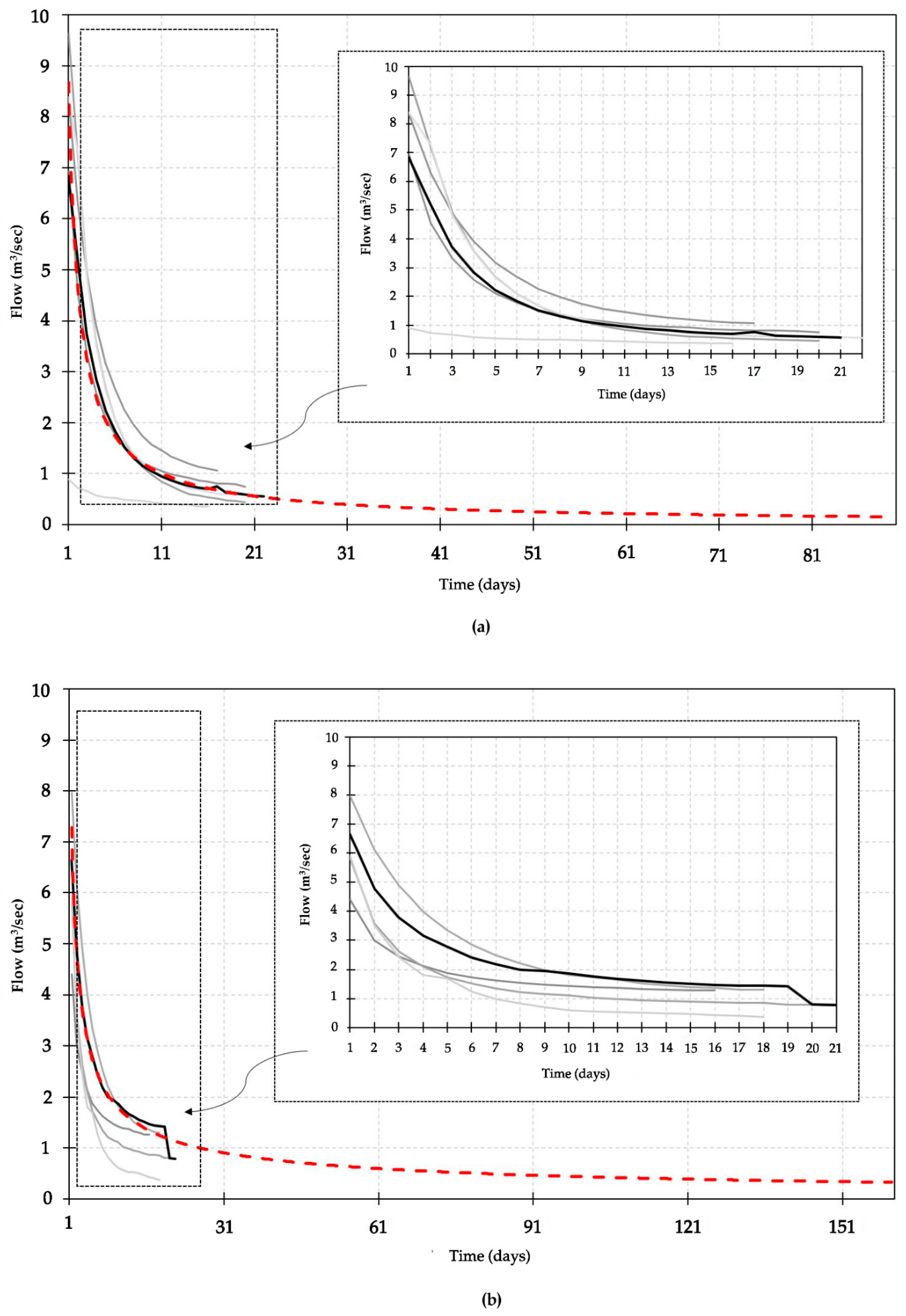
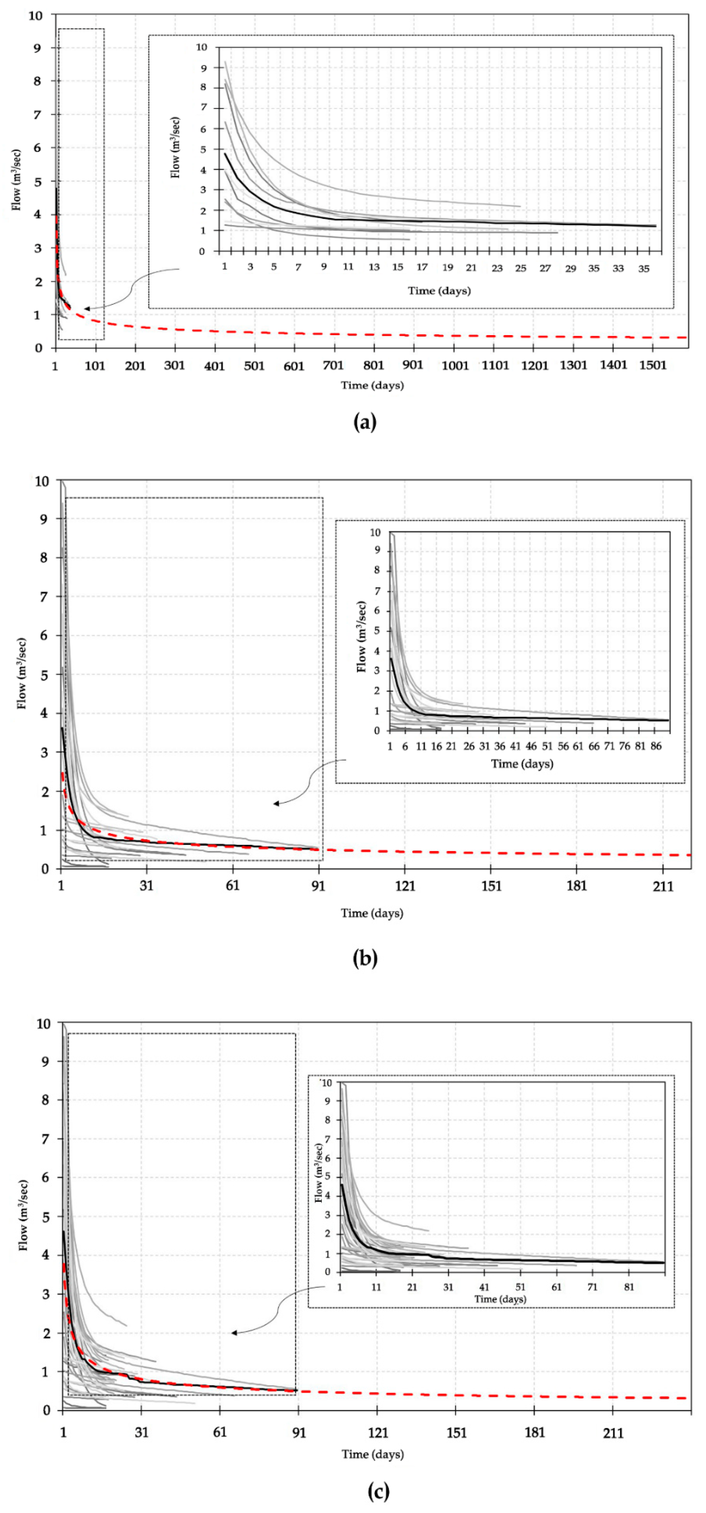
2.3. Description of Flow Recession Curve

The flow recession curve is used widely in hydrologic analysis. After precipitation, surface flow caused by the precipitation in the watershed decreases, along with a base flow consisting mainly of the reservoir water permeated or stored underground, as shown in Equation (5) [31].

$$Q=Q_0{k}^t$$

(5)

where $Q_0$ is the initial flow (m³/s), $Q$ is the flow after $t$ hours (m³/s), and $k$ is the ratio of $Q$ after an hour at $Q_0$, and $t$ is time.

Kullman [39] suggested that during a prolonged period with no or little precipitation, the flow within the watershed declines, as shown in Figure 2. Based on his findings, this study used the daily flow hydrologic curve calibrated for the peak and base flow sections by comparing them with the actual measurements of the SWAT model and assumed that the non-precipitation date is the starting point of the initial flow. In addition, as suggested by Bako and Hunt [37], and Vogel and Kroll [38], recession segments were selected from the daily long-term flow hydrologic curve of the calibrated and validated SWAT model, and each recession segment was analyzed statistically to define the recession curve equation.

2.4. Description of Available Number of Water Intake Days

This paper defined the number of water intake days as the number of days of available flow that can be taken at the water source. This study used and enhanced the recession curve concept proposed by Kullman to calculate the number of water intake days and identify the periods during which the number of days between rainfalls exceeds a certain threshold [39]. The average recession curve of individual recession events was defined (Figure 3) and normalized, and the master recession curve was proposed by extending the curve to the point where the end of the curve meets the drought flow (0.354 m³/s).

In addition, in accordance with the findings of Tallaksen [34] that recession curves progress at different speeds on account of seasonal weather changes, the seasonal recession curves of the study area were defined. Seasons were defined as spring, summer, fall, and winter, and, in accordance with the methods for seasonal meteorological division proposed by Lee [51], the twelve months were grouped into the respective seasons: spring (March to May), summer (June to August), autumn (September to November), and winter (December to February).

The water source’s minimum water intake was defined as the flow until the lowest level that can be taken from the river (local water source) to the water intake station through the intake gate (that is, drought flow). This paper calculated the number of water-intake days in the following steps.

First, this study used the semi-distributed SWAT model to divide sub-watersheds, including the study’s watershed of interest, and calculated daily long-term flow by calibrating and validating the parameters.

Second, the daily long-term flow was used to define a flow recession event with no precipitation and single-out recession segments.

Third, the selected recession events were listed to align the recession curve equations, which were used to calculate the master recession curve equations for the entire period and the respective seasons.

Lastly, considering the drought flows and the water demand for the study water source calculated through the flow analysis using the SWAT model, the available number of water intake days curves was developed.

3. Study Watershed and Materials

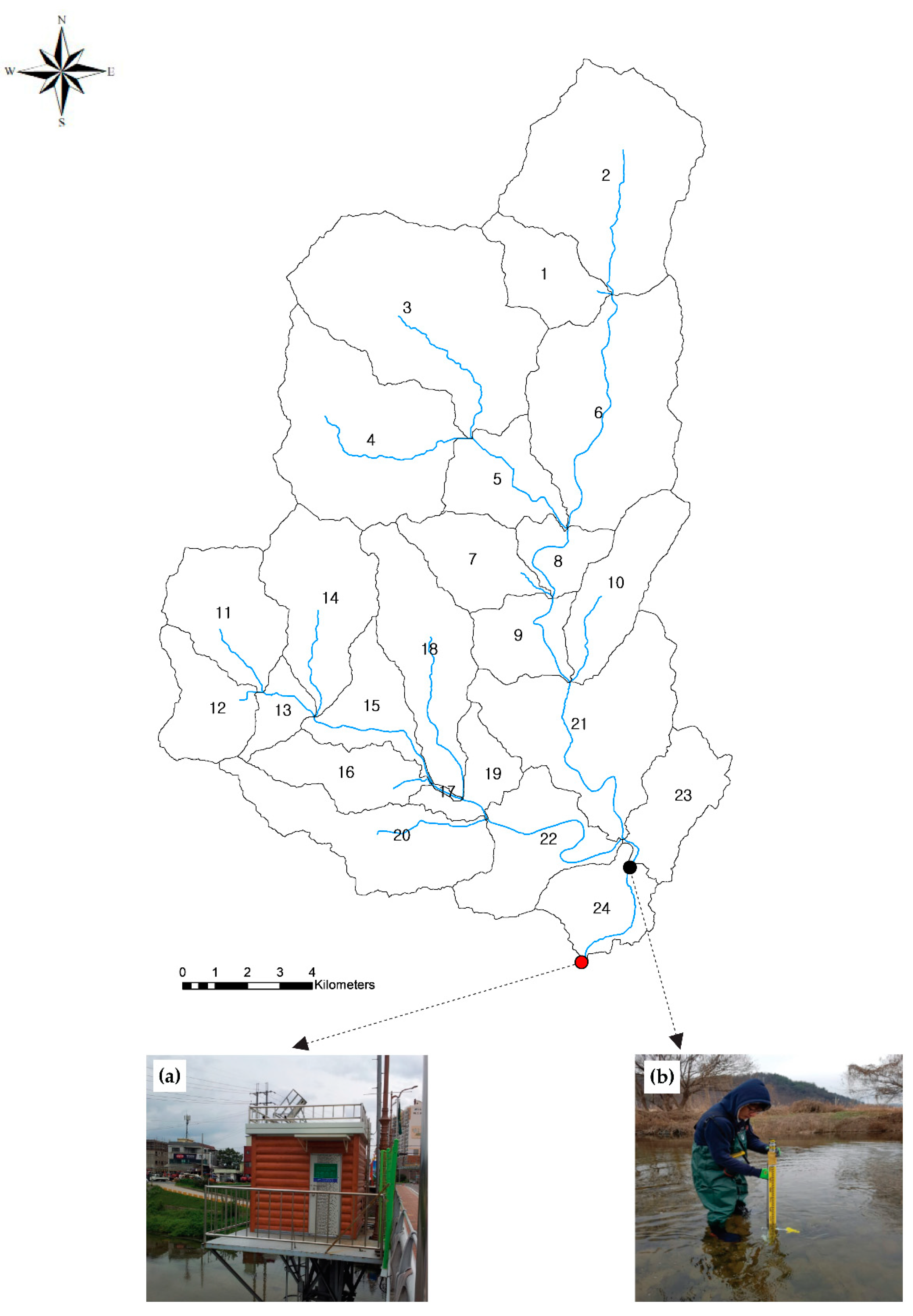
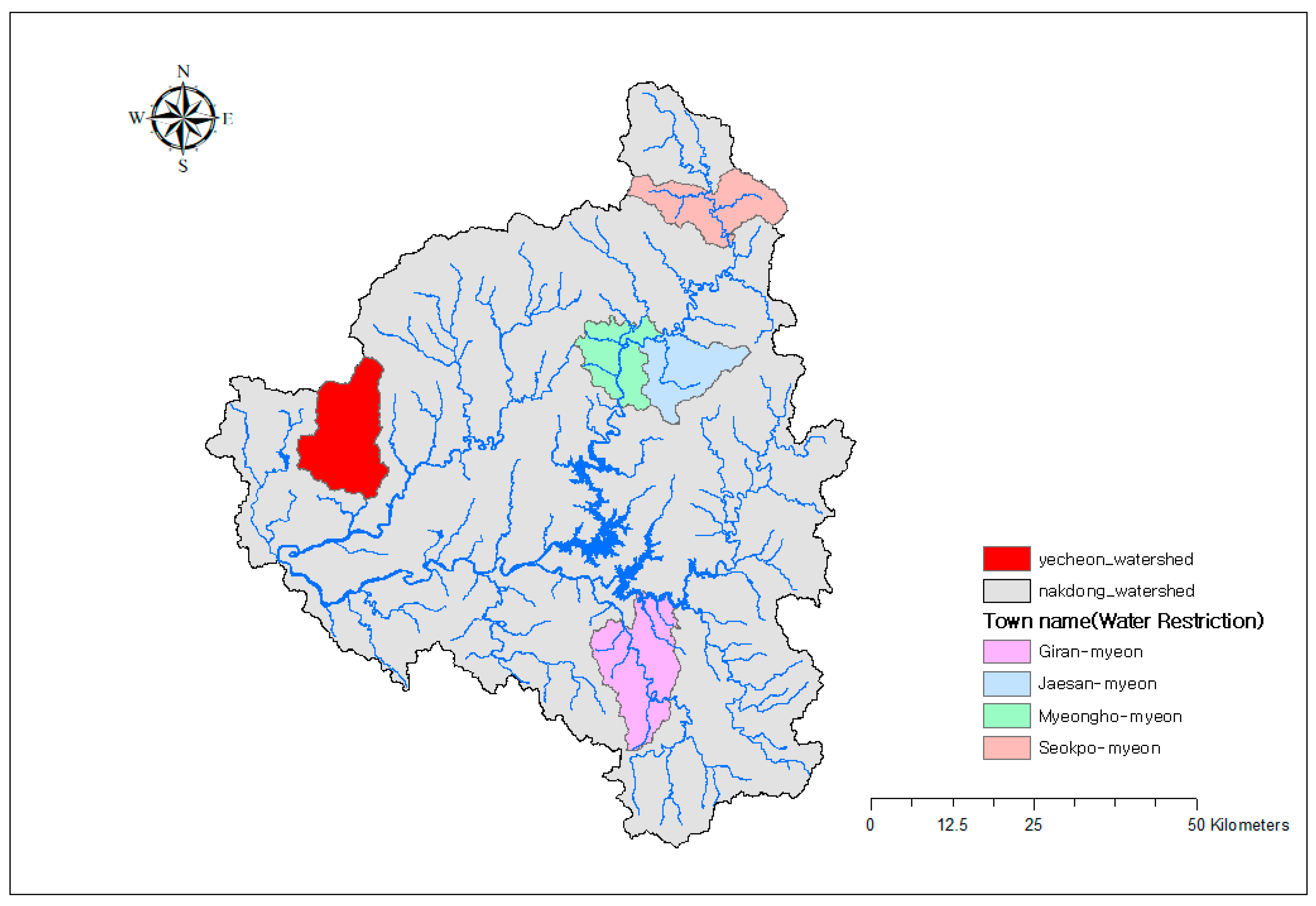
3.1. Selection of the Study Watershed

This study’s watershed of interest is the Hancheon watershed, which is located between 128°37′–128°55′ E, 36°20′–36°28′ N in the Naeseong River section of the Nakdong River System (Figure 4). Its total area is 192.4 km², 29.7 km flow channel extension, an average width of 6.5 km, and a 0.2 watershed shape factor. The watershed at the Yecheon Water Intake Station is located near 432 Baekjeon-ri, Yecheon-gun, Gyeongsangbuk-do, Korea. The station takes riverbed water through concrete collection conduits at the Hancheon River, which serves as the main water source. The Yecheon Water Intake Station, having a capacity of 10,800 m³ per day, supplies to the Yeocheon-eup and Yucheon-myeon areas and the Homyeong-myeon area through the Homyeong Reservoir. In the Yecheon-gun area, the water supply population size is 17,447 persons, and the daily water supply per person stands at 310 L per capita per day (lpcd). The water demand, calculated by multiplying the water supply population with the daily water supply per person, is 4409 m³ per day.

3.2. Meteorological and Hydrologic Data Collection and Organization

3.2.1. Meteorological Data

The framework plan for the Hancheon River and other high-level plans were reviewed to collect meteorological data. The Korea Meteorological Administration (KMA) data regarding the study watershed were reviewed through GIS analysis, and the Yeongju and Mungyeong Weather Stations were selected, from which a 13-year data on daily temperature, precipitation, wind, and humidity were collected (1 January 2006 to 1 January 2018). The analysis found that the average highest temperature in the Yecheon Watershed was 30.1 °C, and the lowest temperature was −7.6 °C. The annual average precipitation and the highest precipitation (in July) were 1274.5 mm and 318.4 mm, respectively. The average humidity was 65%, and the average wind speed was 2.5 m/s (

Table 1. Result weather information construction of Yecheon Basin Area.

Seasonal Classification	Temperature		Precipitation (mm)	Humidity (%)	Wind Speed (m/s)
	Max (°C)	Min (°C)
January	2.6	−7.6	15.0	57.4	3.6
February	5.9	−5.2	33.4	55.1	3.4
March	11.7	−0.4	62.3	55.1	3.2
April	18.3	5.0	98.3	55.3	2.9
May	24.5	10.7	111.0	59.2	2.5
June	27.8	16.0	121.9	67.2	1.9
July	29.1	20.6	318.4	78.4	1.6
August	30.1	20.5	242.3	77.6	1.5
September	25.5	14.3	139.4	76.6	1.6
October	20.3	7.1	61.4	71.5	2.1
November	11.9	0.7	44.3	65.9	2.7
December	4.2	−5.6	26.7	60.8	3.5
Total Period	17.7	6.3	1274.5	65.0	2.5

).

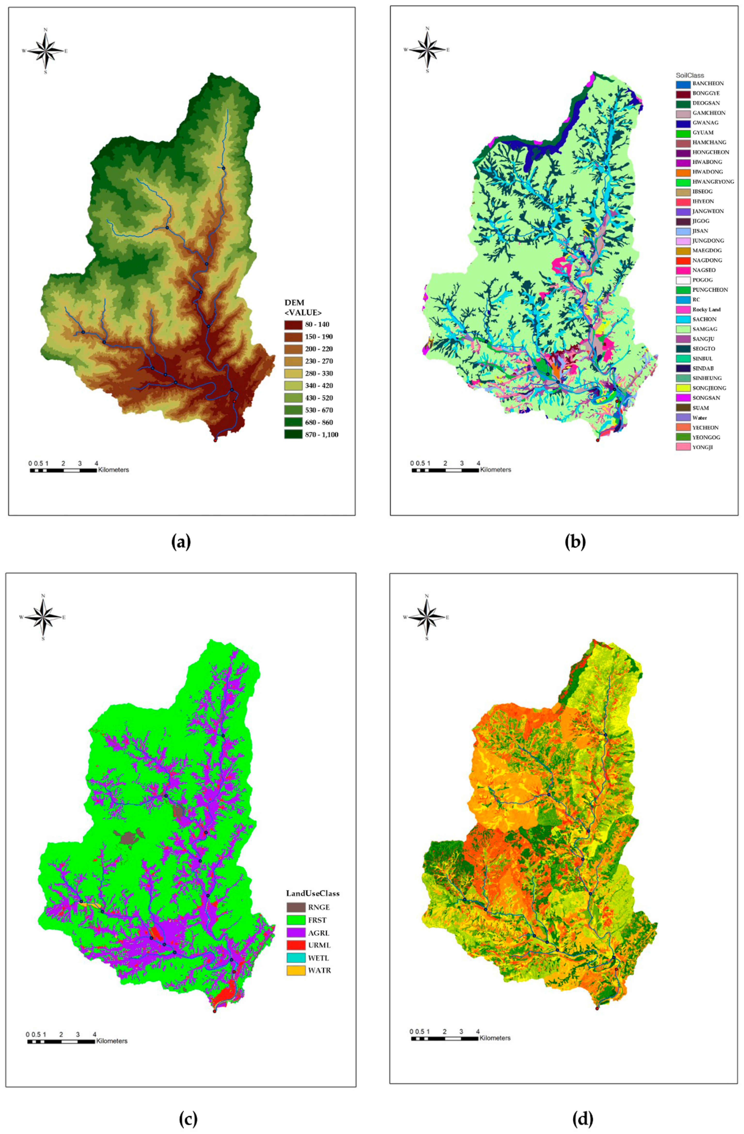
3.2.2. Geographical Information System (GIS) Data

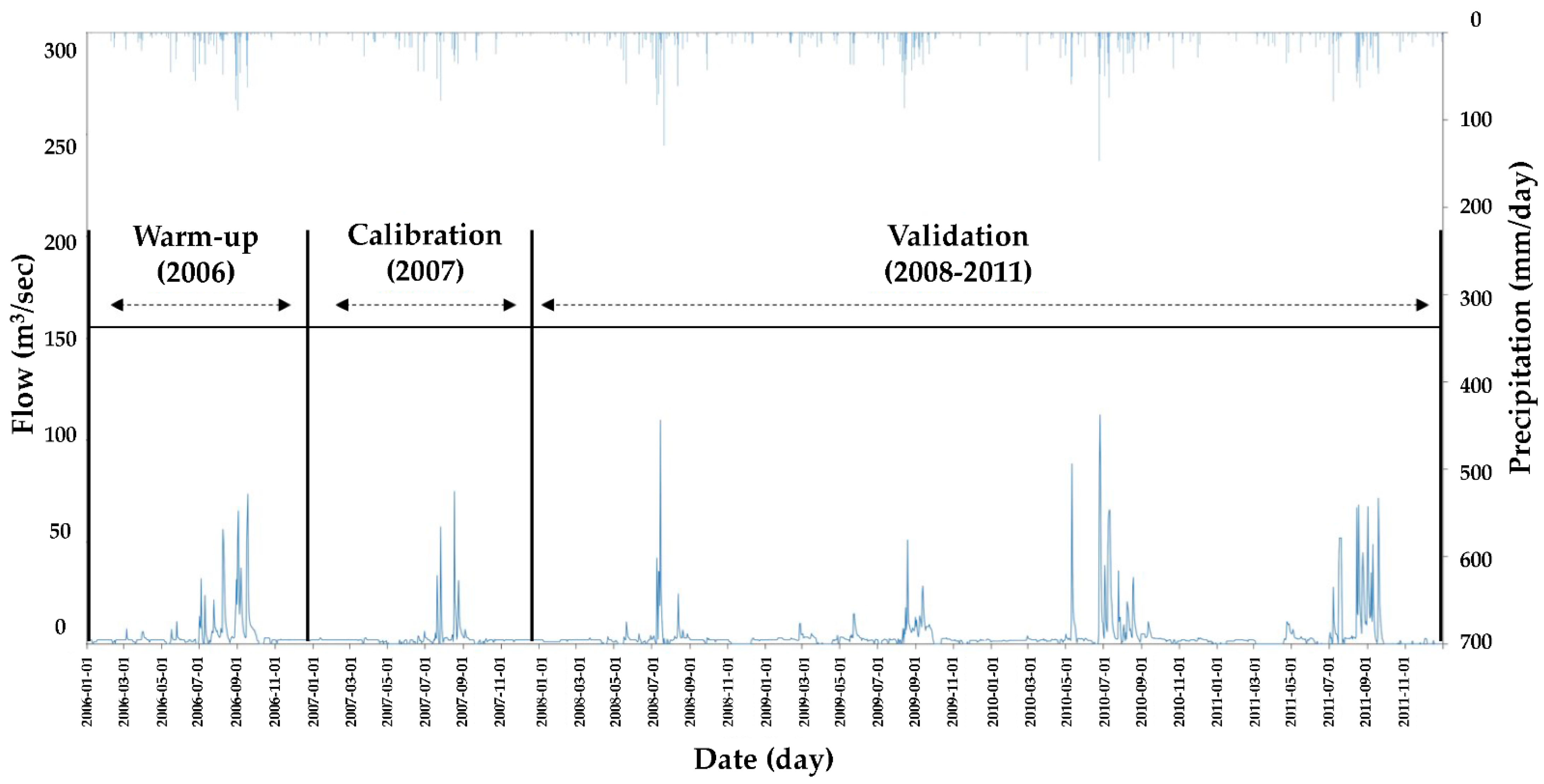
This study put together a soil map, a land use map, and topographical data, such as digital elevation model (DEM) data, to operate the SWAT model. The highest, lowest, and average DEM of the Yecheon Watershed derived through the watershed division were 1100 m, 79 m, and 381 m, respectively (Figure 5a). The soil map plays a crucial role in the surface flow, evaporation, and circulation of soil water and underground water in the SWAT model. This study used the 1:25,000 scale soil map provided by the Rural Development Administration (RDA) to build input data for the SWAT model in the GIS format (Figure 5b). In addition, the soil properties, encroachments, effective soil depths, and drainage grades derived from the RDA’s Soil Environment Information System [52] were matched with the soil information, and the soil moisture and field capacity were calculated using the soil property estimation method proposed by Saxton et al. [53]. In the soil map developed for the Yecheon Watershed, the soil series distribution rates were 59.8% for SAMGAG (mountain and forest soil, granite, and granite-Gneiss), 14.2% for SEOGTO (upland soil, granite, and granite-gneiss), and 7.5% for SACHON (paddy soil, granite, and granite-gneiss). As for the land use map, this study used the 1:25,000 land cover map provided by the ME Environmental Geographical Information System [54], and the ME’s land use classifications were reorganized in alignment with the SWAT model input codes. The reorganization results are shown in Figure 5c. In the land use map, mixed forests accounted for the highest percentage (68.6%), followed by crop fields (26.4%), residential areas (2.6%), other green lands (1.5%), marshes (0.4%), and basins (0.5%). The inclines of the watershed were calculated from the DEM. Inclines were categorized into three groups: 0–30; 30–60; and higher than 60. The percentage of the 30–60 inclines was the highest at 51%, followed by 0–30 (37%), and higher than 60 (12%). The incline map, soil map, and land use map were used to calculate the SWAT model’s hydrologic response units (HRUs), which resulted in 2,274 HRUs (Figure 5d).

3.2.3. Flow Data

The Yecheon Water Level Gauging Station of the MOE Nakdong River Flood Control Office is located 2 km downstream from the Yecheon Water-Intake Station, at around 310-19 (Yecheongyo Bridge) Nambon-ri, Yecheon-eup, Yecheon-gun, Gyeongsangbuk-do, Korea. The Yecheon Water Level Gauging Station measures water level with T/M equipment. The station holds daily data from January 1963 to 2020. Despite the long period of measurement, the station lacks flow measurement data. Data before 2007 are not available because of the opening of weir gates. For this reason, this study selected the daily flow data calculated with the 2007 water level flow rating curve equation proposed in the Hydrologic Annual Report, except for the data on the days when the weir gates were open.

Even though a water level gauging station in the downstream section of the Hancheon River exists, this study conducted on-site measurement of flow rates to determine drought flow at the water-intake source, calculate the drought reference values (drought water level and drought flow), and collect the water level and flow data used for the validation of the SWAT model. Specifically, depths and flow rates were calculated based on the number of verticals. Flow rates were calculated using the midsection method, which calculates the flow rates and sectional areas of the segments, other than the first and the last segments, and sums up the respective segments’ flow rates.

Table 2. Results of the on-site flow measurement.

Date	Measurement Flow (m3/s)	Daily Average Flow (m3/s)
7 December 2016	0.514, 0.511	0.513
11 January 2017	0.579, 0.581	0.580
7 February 2017	0.470, 0.442	0.456
16 March 2017	0.556, 0.544	0.550
11 April 2017	2.680, 2.637, 2.699, 2.653	2.667

shows the flow measurement results between December 2016 and April 2017. Measurements were taken two to four times at certain intervals depending on the situation on-site.

3.3. Division of Subbasins

The DEM is a crucial element in determining the shape of a watershed and water movement direction. This study extracted the 7111 (intermediate contour: 2 m) and the 7114 (index contour: 10 m) from the 1:5000 digital evaluation map from the National Geographic Information Institute (NGII) and converted them to 5 m resolution GIS Raster files. The converted DEM data were then used to analyze the flow direction and accumulation of the river to create a river network. Then, 24 sub-watersheds were identified by setting two flow observation points: the Yecheon Water-Intake Station and the MOE Water Level Gauging Station (Yecheon Bridge) (Figure 6).

4. Application and Analysis

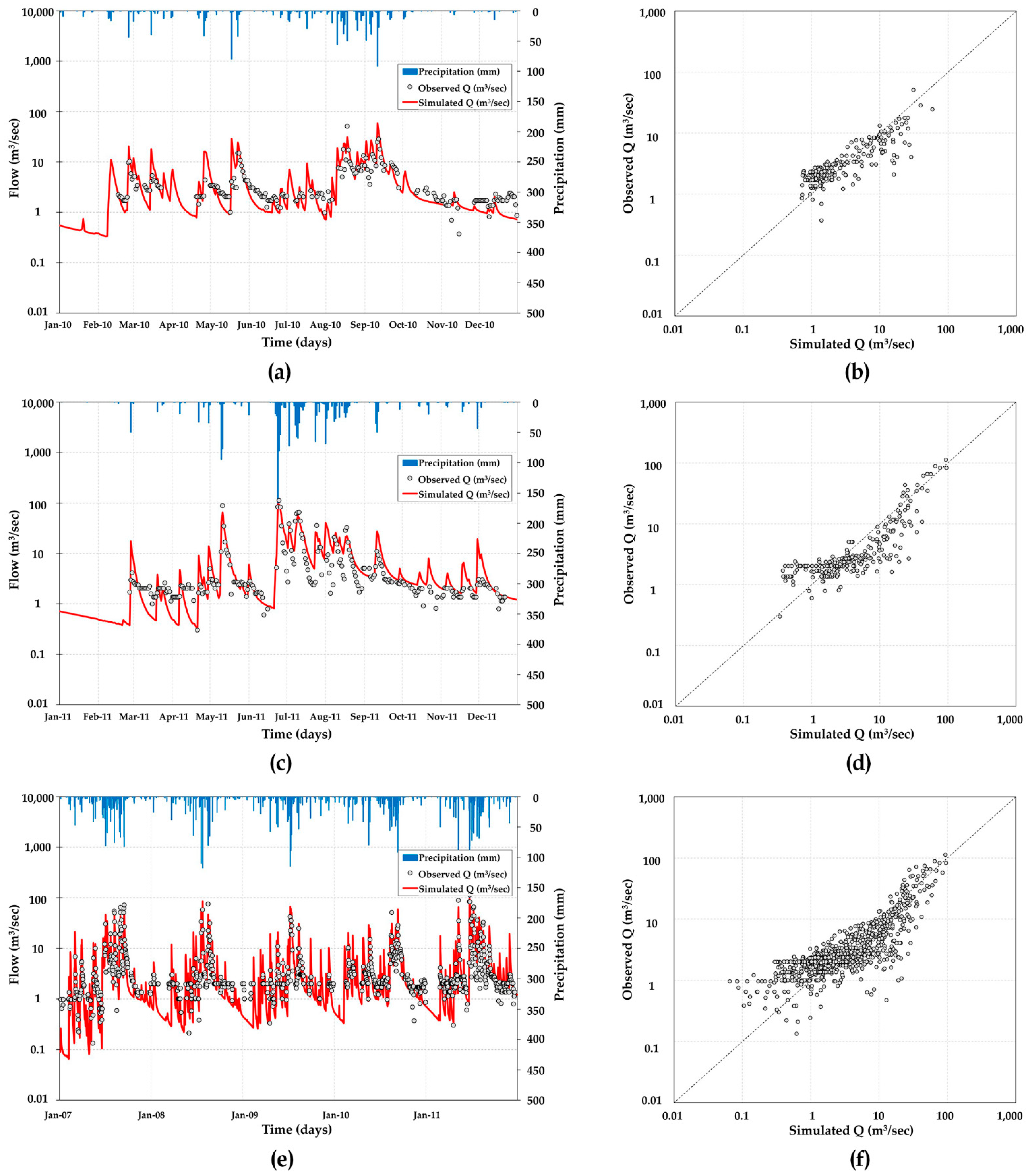
4.1. Calculation of Long-Term Flow Using the SWAT Model

This study reviewed the 10-year water level and flow data at the MOE Yecheon Water Level Gauging Station to acquire reliable daily flow data and determined whether a water level flow rating curve exists. For this study, the 2007 water level data were determined to be available for removing artificial factors, such as the opening of weir gates, and the water level flow rating curve equation was used to calculate daily flow rates. To calibrate the flow rate parameter, as shown in Figure 7, the year 2006 was selected as the warm-up period, and the calibration period (2007) and the validation period (2008–2011) were likewise defined.

Three parameters affecting the surface, interim, and baseflow, respectively, were selected from previous studies and the SWAT manual for parameter calibration (CN2, ESCO, CANMX, SOL_K, SLSOIL, LAT_TIME, GW_DELAY, GWQMN, ALPHA_BF). After analyzing each parameter’s sensitivity, five of them were selected for the study, as shown in

Table 3. Selected value for explanation and calibration of Soil and Water Assessment Tool (SWAT) model parameters.

Parameters	Definition	Default	Range	Calibrated Values
CN2	SCS curve number for moisture condition	Various	35 to 98	−25%
ESCO	Soil evaporation compensation coefficient	0.95	0 to 1	0.1
GW_DELAY	Delay time for aquifer recharge (days)	31	0 to 500	80
ALPHA_BF	Base flow recession constant (days)	0.048	0 to 1	0.8
GWQMN	Threshold water level in shallow aquifer for baseflow (mm)	1000	0 to 5000	2000

(CN2, ESCO, GW_DELAY, GWQMN, ALPHA_BF). Then, the peak segment of the flow curve was calibrated closer to the actual measurements. The flow rates in the early conditions were overestimated above the actual measurements. The CN2 value, which represents the SCS flow curve indicator in AMC-2, was reduced by 25%, and the soil evaporation compensation factor (ESCO) was lowered from the initial 0.95 to 0.1 to address the issue. Using the calibrated parameters, the flow at the recession segment in the flow curve was adjusted closer to the actual measurement. To that end, the delay time for aquifer recharge was extended from 31 to 80 days. In addition, the base flow recession constant was raised from 0.048 day to 0.8 day, and the threshold water level in a shallow aquifer for base flow was raised from 1000 mm to 2000 mm by 50 mm increments.

The calibration resulted in that the daily flow hydrologic curves and the scatterplot graphs are shown in Figure 8a,b, which follow the overall actual measurements’ tendencies.

The determination coefficient for comparing the true and predicted values of the SWAT model in 2007 ($R^2$) was 0.89, which is “very good” according to the statistical performance assessment criteria proposed by Moriasi et al. [50]. The value of NSE, which compares the reflection of tendencies between the true and predicted values of the SWAT model, was 0.88, which is “very good.” In addition, PBIAS, which compares the sums of the true and predicted values of the SWAT model, was –3.1%, which is within 5% of the total and classified as “very good.” The findings confirm that the parameter calibration of the SWAT model was carried out appropriately.

Then, this study applied the parameters calibrated for 2007 to the 2008–2011 period. The calibration for the 2008–2011 period resulted in the time-series graphs of the daily flow hydrologic curves are in Figure 8c,e to Figure 8a,c, which follow the tendencies of the overall actual measurements. The scatterplot graphs are shown in Figure 8d,f to Figure 8b,d, which are similar to the parameter-adjusted graphs. The determination coefficients ($R^2$) of the SWAT model were 0.92, 0.97, 0.93, and 0.89 in each year from 2008 to 2011, NSE were 0.67, 0.96, 0.82, and 0.86, and PBIAS were 8.3, 3.1, 13.7, and 14.2 m, which represent good results.

Figure 9e,f show the daily flow hydrologic curves and scatterplot graphs between 2007 and 2011. Throughout the calibration/validation period, the average determination coefficient ($R^2$) was 0.92 and NSE was 0.84, which are “very good” under the statistical performance assessment criteria. PBIAS was 7.24%, which is “good” under the statistical performance assessment criteria. The average annual precipitation was 1255 mm, and the total flow was 697 mm or 56% of the precipitation. The evapotranspiration was 495 mm or 39% of the precipitation. In the SWAT model, the total flow is the sum of the direct and indirect flow. The annual average of direct flow was 532 mm or 42% of the precipitation, and the annual average indirect flow was 165 mm or 13% of the precipitation.

A comparison of the flow measurements between December 2016 and May 2017 at the Yecheon Water Intake Station verified that the absolute values and tendencies are similar. In addition, an analysis of the water flow in the study watershed (Yecheon Water-Intake Station) using the long-term (10 years, 2007–2017) flow derived from the SWAT model, the abundant flow rate was 3.728 m³/s, the normal flow was 1.521 m³/s, the low flow rate was 0.778 m³/s, and the drought flow rate was 0.354 m³/s (

Table 4. Results of flow-duration analysis for Yecheon Water Intake Station and Yecheon Bridge.

Duration Curve Zone	Yecheon Water-Intake Station (m3/s)	Yecheon Bridge (m3/s)
Moist conditions	3.728	3.830
Midrange flows	1.521	1.590
Dry conditions	0.778	0.815
Low flow	0.354	0.373

). Figure 10 shows the flow comparison between the Yecheon Water Intake Station and the Yecheon Bridge.

4.2. Calculation Results of Water Supply Available Days Curve

Based on the daily long-term flow data from the calibrated and validated SWAT model, the recession events with 15 or more days of recession without precipitation were identified using the recession curve concept proposed by Kullman [39]. To that end, this study used the daily long-term flow calculations at the Yecheon Water Intake Station between 2007 and 2017, which resulted in 43 recession events. The 43 events were distributed across the four seasons as proposed by Tallaksen [34]. Five events were identified between March and May, which were used to define the master recession curve equation for spring and the determination coefficient ($R^2$ = 0.99). The master recession curve equation for each season was calculated using the same method, as shown in Figure 11 and Figure 12.

Table 5. Result of calculating the available number of water-intake days curve equation.

Seasonal Classification	$\mathbf{Coefficient}\mathbf{of}\mathbf{Determination}\left({\mathit{R}}^2\right)$	Master Recession Curve Equation
Spring (March–May)	0.99	$Q=8.6807{\left(days\right)}^{-0.9}$
Summer (June–August)	0.93	$Q=7.2874{\left(days\right)}^{-0.611}$
Autumn (September–November)	0.94	$Q=3.9429{\left(days\right)}^{-0.343}$
Winter (December–February)	0.91	$Q=2.4698{\left(days\right)}^{-0.356}$
Total Period (January–December)	0.98	$Q=3.7768{\left(days\right)}^{-0.45}$

lists the determination coefficient and the available number of water-intake days curve equation for each season. The calculation found that the curves are steeper in spring and summer and slower in autumn and winter. The overall determination coefficient was 0.98. By season, the winter determination coefficient was the highest at 0.91, followed by summer (0.93), autumn (0.94), and spring (0.99).

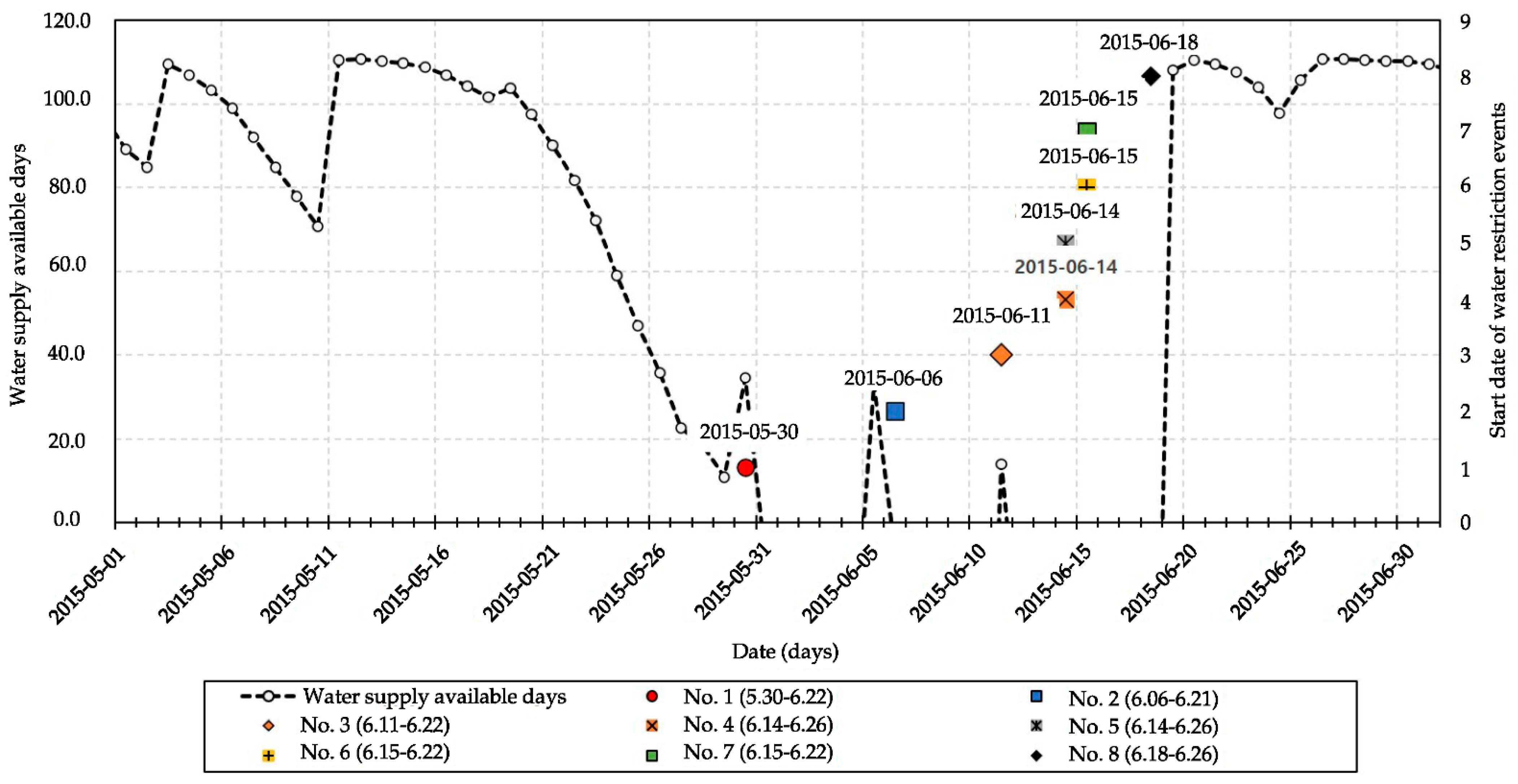
4.3. Comparison of Drought Cases and Applicability Evaluation

Based on the water supply restriction in the Nakdong River Watershed, which includes the Yecheon Watershed, this study determined the number of days of water supply restriction in May and June 2015 (Figure 13,

Table 6. Status of damages from water restriction at Nakdong River Basin covering the study area (2015).

No.	Town Name	Water Restriction Events (Date)	Household	Water Supply Population
1	Giran-myeon	June 18–26	17	32
2	Jaesan-myeon	June 15–22	8	20
3	Jaesan-myeon	June 15–22	8	20
4	Myeongho-myeon	June 14–26	3	10
5	Myeongho-myeon	June 14–26	8	20
6	Myeongho-myeon	June 11–22	11	18
7	Seokpo-myeon	June 6–21	14	21
8	Jaesan-myeon	May 30–June 22	18	40

). Then, the findings were used to compare the time series of the available number of water intake derived from the available number of water-intake days curves. The findings are as shown in Figure 14. All water supply restriction cases began in the May 31–June 18 period, when the available number of water-intake days in the Yecheon Watershed dropped below the dry season level. The findings indicate a high level of accuracy, which suggests a high level of applicability.

5. Conclusions

The purpose of this study was to provide information for drought response and water resource planning aimed at effectively preventing the inconvenience and financial damage caused by water supply restrictions at local water sources on account of droughts and water shortage. Visits to local waterwork sites revealed that the personnel in the field are in need of the data on the number of days that water can be taken from the water source in case of no precipitation. Therefore, this study sought to develop a methodology for determining the available number of water-intake days quantitatively to ensure the local waterworks’ resilience against droughts. The details and findings of this study are summarized below.

First, the SWAT model was used to calibrate and validate the daily flow hydrologic curve, which resulted in the determination coefficients for the total period ($R^2$), NSE, and PBIAS at 0.70, 0.54, and 12.9, respectively, which fall under the “satisfactory” category based on the statistical performance assessment criteria proposed by Moriasi et al. [50]. The water balance of the study watershed was analyzed based on these findings, and the average annual precipitation was 1255 mm, while the total flow was 697.4 mm or 55.6% of the precipitation. The evapotranspiration was 495.2 mm or 39.4% of the precipitation.

Second, based on the daily long-term flow at the MOE’s local water source for the 2007–2017 period calibrated and validated using the SWAT model, the recession curve concept proposed by Kullman [39] was used to identify the periods of the recession events with 15 or more days of recession without precipitation. Based on the 43 precipitation events and the effect of seasonal weather proposed by Tallaksen [34], the available number of water intake days curves were calculated, accounting for the daily average water demands and drought flow rates throughout the total period and each season.

Third, this study applied the available number of water intake days curve equation developed for the local water source to actual cases of water supply restrictions in the study area and found that the starting dates of water supply restriction and the available numbers of water intake days matched the periods in which the water level dropped below the dry season level. In addition, this study proposed practical and straightforward concepts that can be used by local water source staff to respond to droughts.

In this paper, a practical and straightforward indicator for drought response in case of no rainfall used at the water intake station was developed, which was not be presented in previous studies. However, this study needs to be supplemented by further research on applying the methodology developed in this study to various areas and cases. Once optimized for different areas, the methodology is expected to be applicable to drought response and water resource planning to effectively prevent the inconvenience and financial damage caused by water supply restriction at local water sources on account of droughts and water shortage.

References

1. Bekele, E.G.; Knapp, H.V. Watershed modeling to assessing impacts of potential climate change on water supply availability. Water Resour. Manag. 2010, 24, 3299–3320. [Google Scholar] [CrossRef]
2. Muttiah, R.S.; Wurbs, R.A. Modeling the impacts of climate change on water supply reliabilities. Water Int. 2009, 22, 407–419. [Google Scholar] [CrossRef]
3. Ministry of Land, Infrastructure and Transport (MOLIT). Long-Term Water Resource Management Master Plan (2011–2020); MOLIT: Gwacheon, Korea, 2011. Available online: https://dl.nanet.go.kr/file/fileDownload.do?linkSystemId=NADL&controlNo=MONO1201205881 (accessed on 17 April 2020). (In Korean)
4. Ministry of Environment (ME); Korea Water Resources Corporation (K-Water). Drought Report Survey in 2019; ME: Sejong, Korea, 2019. Available online: https://dl.nanet.go.kr/file/fileDownload.do?linkSystemId=NADL&controlNo=MONO1202028920 (accessed on 15 February 2021). (In Korean)
5. Kim, T.W.; Park, D.H. Guidelines for extreme drought planning adaptation to climate change. J. Korean Soc. Civ. Eng. 2018, 66, 43–48. [Google Scholar]
6. Ministry of Environment (ME). A Study on the Development of Drought Prediction and Response System for Local Water Supply System; ME: Sejong, Korea, 2017. Available online: https://dl.nanet.go.kr/file/fileDownload.do?linkSystemId=NADL&controlNo=NONB1301902785 (accessed on 20 April 2020). (In Korean)
7. Ministry of Construction and Transport (MOCT); Korea Water Resources Corporation (K-Water). Long-Term Water Resource Management Master Plan (2006–2020); MOCT: Gwacheon, Korea, 2006. Available online: https://dl.nanet.go.kr/file/fileDownload.do?linkSystemId=NADL&controlNo=MONO1200721496 (accessed on 17 April 2020). (In Korean)
8. Ryu, J.N. Review of Water Budget Management Methods Using Causal Loop; Korea Environment Institute (KEI): Sejong, Korea, 2015; Available online: https://library.kei.re.kr:444/dmme/img/001/012/004/%ea%b8%b0%ec%b4%882015_12_%eb%a5%98%ec%9e%ac%eb%82%98.pdf (accessed on 12 March 2020). (In Korean)
9. Ministry of Construction and Transport (MOCT). Long-Term Water Resource Management Master Plan (Water Vision 2020); MOCT: Gwacheon, Korea, 2001. Available online: https://dl.nanet.go.kr/file/fileDownload.do?linkSystemId=NADL&controlNo=MONO1200111563 (accessed on 17 April 2020). (In Korean)
10. Ministry of Environment (ME). Comprehensive Plan on National Water Demand Management; ME: Sejong, Korea, 2007. Available online: https://dl.nanet.go.kr/file/fileDownload.do?linkSystemId=NADL&controlNo=NONB1200729862 (accessed on 12 March 2020). (In Korean)
11. Kim, H. A Study on Adaptive Drought Management Policy to Drought Stages: Focused on the Non-Structural Measures at Local Scale; Korea Environment Institute (KEI): Sejong, Korea, 2016; Available online: https://library.kei.re.kr:444/dmme/img/001/011/006/%ec%88%98%ec%8b%9c2016_01_%ea%b9%80%ed%98%b8%ec%a0%95.pdf (accessed on 17 April 2020). (In Korean)
12. Chung, I.M.; Lee, J.W.; Lee, J.E.; Choi, J.R. The estimation of sand dam storage using a watershed hydrologic model and reservoir routing method. J. Eng. Geol. 2018, 28, 541–552. [Google Scholar]
13. Choi, J.R.; Chung, I.M.; Jo, H.J. A study on the establishment of water supply and demand monitoring system and drought response plan of small-scale water facilities. J. Eng. Geol. 2019, 29, 469–481. [Google Scholar]
14. Rockwood, D.M.; Davis, E.M.; Andersen, J.A. User’s Manual for COSSARR: A Digital Computer Program Designed for Small to Medium Scale Computers Performing Streamflow Synthesis and Reservoir Regulation in Conversational Mode; U.S. Army Engineering: Division, OR, USA, 1972.
15. Sugarawa, M.; Ozaki, E.; Watanabe, I.; Katsuyama, Y. Tank model and its application to Bird Creek, Wollombi Brook, Bihin River, Kitsu River, Sanaga River, and Nam Mune. In Research Notes of National Center for Dister Prevention (NCDP) 11; NCDP: Tokyo, Japan, 1976; pp. 1–64. [Google Scholar]
16. Beven, K.J.; Kirby, M.J. A physically-based variable contributing area model of basin hydrology. Hydrol. Sci. Bull. 1979, 24, 46–69. [Google Scholar] [CrossRef] [Green Version]
17. Arnold, J.G.; Allen, P.M.; Bernhardt, G. A comprehensive surface-groundwater flow model. J. Hydrol. 1993, 142, 47–69. [Google Scholar] [CrossRef]
18. Beven, K.J.; Kirkby, M.J.; Schofield, N.; Tagg, A.F. Testing a physically based flood forecasting model (TOPMODEL) for three UK catchments. J. Hydrol. 1984, 69, 119–143. [Google Scholar] [CrossRef]
19. Kim, H.Y.; Park, S.W. Simulating daily inflow and release rates for irrigation reservoirs, 1: Modeling inflow rates by a linear reservoir model. J. Korean Soc. Agric. Eng. 1988, 30, 50–62. [Google Scholar]
20. Arnold, J.G.; Williams, J.R.; Srinivasan, R.; King, K.W.; Griggs, R.H. SWAT: Soil Water Assessment Tool; U.S. Department of Agriculture, Agricultural Research Service, Grassland, Soil and Water Research Laboratory: Temple, TX, USA, 1994.
21. Song, J.H. Hydrologic Analysis System with Multi-Objective Optimization for Agricultural Watersheds. Ph.D. Thesis, Seoul National University, Seoul, Korean, 2017. [Google Scholar]
22. Leta, O.T.; Bauwens, W. Assessment of the impact of climate change on daily extreme peak and low flows of Zenne Basin in Belgium. Hydrology 2018, 5, 38. [Google Scholar] [CrossRef] [Green Version]
23. Sehgal, V.; Sridhar, V. Effect of hydroclimatological teleconnections on the watershed-scale drought predictability in the southeastern United States. Int. J. Climatol. 2018, 38, e1139–e1157. [Google Scholar] [CrossRef]
24. Hoyos, N.; Correa-Metrio, A.; Jepsen, S.M.; Wemple, B.; Valencia, S.; Marsik, M.; Doria, R.; Escobar, J.; Restrepo, J.C.; Velez, M.I. Modeling streamflow response to persistent drought in a coastal tropical mountainous watershed, Sierra Nevada De Santa Marta, Colombia. Water 2019, 11, 94. [Google Scholar] [CrossRef] [Green Version]
25. Le, M.H.; Lakshmi, V.; Bolten, J.; Bui, D.D. Adequacy of satellite-derived precipitation estimate for hydrological modeling in Vietnam basins. J. Hydrol. 2020, 586, 124820. [Google Scholar] [CrossRef]
26. Kumar, A.; Sharma, M.P. A modeling approach to assess the greenhouse gas risk in Koteshwar hydropower reservoir, India. Hum. Ecol. Risk Assess. 2016, 22, 1651–1664. [Google Scholar] [CrossRef]
27. Senent-Aparicio, J.; Alcalá, F.J.; Liu, S.; Jimeno-Sáez, P. Coupling SWAT model and CMB method for modeling of high-permeability bedrock basins receiving interbasin groundwater flow. Water 2020, 12, 657. [Google Scholar] [CrossRef] [Green Version]
28. Wilhite, D.A.; Glantz, M.H. Understanding the drought phenomenon: The role of definitions. Water Int. 1985, 10, 111–120. [Google Scholar] [CrossRef] [Green Version]
29. An, B.K.; Kim, T.C.; Park, S.K.; Lee, K.G. A study on the variation of recession constants in daily hydrographs. J. Korean Soc. Agri. Eng. 1991, 33, 45–54. [Google Scholar]
30. Boussinesq, J. Sur un mode simple d’ecoulement des nappes d’eau d’infiltration a lit horizontal, avec rebord vertical tout autour lorsqu’une partie de ce rebord est enlevee depuis la surface jusqu’au fond. CR Acad. Sci. 1903, 137, 5–11. (In French) [Google Scholar]
31. Barnes, B.S. The structure of discharge recession curve. Eos Trans. AGU 1939, 20, 721–725. [Google Scholar] [CrossRef]
32. Hall, F.R. Base-flow recession—A review. Water Resour. Res. 1968, 4, 973–983. [Google Scholar] [CrossRef]
33. Nathan, R.J.; McMahon, T.A. Evaluation of automated techniques for base flow and recession analysis. Water Resour. Res. 1990, 26, 1465–1473. [Google Scholar] [CrossRef]
34. Tallaksen, L.M. A review of baseflow recession analysis. J. Hydrol. 1995, 165, 349–370. [Google Scholar] [CrossRef]
35. Klaasen, B.; Pilgrim, D.H. Hydrograph recession constants for New South Wales stream. Civil. Eng. Trans. Inst. Eng. 1975, CE17, 43–49. [Google Scholar]
36. Singh, K.P. Some factors affecting base flow. Water Resour. Res. 1968, 4, 985–999. [Google Scholar] [CrossRef]
37. Bako, M.D.; Hunt, D.N. Derivation of baseflow recession constant using computer and numerical analysis. Hydrol. Sci. J. 1988, 33, 357–367. [Google Scholar] [CrossRef]
38. Vogel, R.M.; Kroll, C.N. Regional geohydrologic-geomorphic for the estimation of low-flow statics. Water Resour. Res. 1992, 28, 2451–2458. [Google Scholar] [CrossRef]
39. Kullman, E. Krasovo–Puklinové Vody—Karst-Fissure Waters; Geologický ústav Dionýza Štúra: Bratislava, Slovakia, 1990; p. 184. [Google Scholar]
40. Jeon, M.W.; Jeon, S.H.; Cho, Y.S. Determining parameters of storage function runoff model from recession curve. J. Inst. Constr. Technol. 2000, 19, 141–152. [Google Scholar]
41. Kim, D.R.; Kim, S.J. A study on parameter estimation for SWAT calibration considering streamflow of long-term drought periods. J. Korean Soc. Agric. Eng. 2017, 59, 19–27. [Google Scholar] [CrossRef] [Green Version]
42. Lee, J.C.; Park, Y.K.; Jung, J.S. A study on estimation of recession constant in base flow. J. Korean Soc. Environ. Technol. 2001, 2, 7–15. [Google Scholar]
43. Kienzle, S.W. The use of the recession index as an indicator for streamflow recovery after a multi-year drought. Water Resour. Manag. 2006, 20, 991–1006. [Google Scholar] [CrossRef]
44. Fiorotto, V.; Caroni, E. A new approach to master recession curve analysis. Hydrol. Sci. J. 2013, 58, 966–975. [Google Scholar] [CrossRef] [Green Version]
45. Kim, C.G.; Kim, N.W. Comparison of natural flow estimates for the Han River basin using TANK and SWAT models. J. Korea Water Resour. Assoc. 2012, 45, 1226–6280. [Google Scholar] [CrossRef] [Green Version]
46. Han, J.H.; Ryu, T.S.; Lim, K.J.; Jung, Y.H. A review of baseflow analysis techniques of watershed-scale runoff models. J. Korean Soc. Agric. Eng. 2016, 58, 75–83. [Google Scholar] [CrossRef] [Green Version]
47. Williams, J.R.; Nicks, A.D.; Arnold, J.G. Simulator for water resources in rural basins. J. Hydraul. Eng. 1985, 111, 970–986. [Google Scholar] [CrossRef]
48. Arnold, J.G.; Williams, J.R.; Nicks, A.D.; Sammons, N.B. SWRRB: A Basin Scale Simulation Model. for Soil and Water Resources Management; Texas A & M University Press: College Station, TX, USA, 1990. [Google Scholar]
49. Neitsch, S.L.; Arnold, J.G.; Kiniry, J.R.; Williams, J.R. Soil and Water Assessment Tool Theoretical Documentation Version 2009; Texas Water Resources Institute: College Station, TX, USA, 2011. [Google Scholar]
50. Moriasi, D.N.; Gitau, M.W.; Pai, N.; Daggupati, P. Hydrologic and water quality models: Performance measures and evaluation criteria. Trans. ASABE 2015, 58, 1763–1785. [Google Scholar] [CrossRef] [Green Version]
51. Lee, B.S. A study of natural seasons in Korea. J. Korean Geogr. Soc. 1979, 20, 1–11. [Google Scholar]
52. Rural Development Administration (RDA). Soil Environment Information System. Available online: http://www.rda.go.kr/foreign/ten/ (accessed on 2 December 2017).
53. Saxton, K.E.; Rawls, W.J.; Romberger, J.S.; Papendick, R.I. Estimating generalized soil-water characteristics from texture. Soil Sci. Soc. Am. J. 1986, 50, 1031–1036. [Google Scholar] [CrossRef]
54. Ministry of Environment (ME). Environmental Geographical Information System. Available online: https://egis.me.gov.kr (accessed on 2 December 2017).
Figure 1. Flow chart of the study.
Water 13 01511 g001
Figure 2. Definition of recession curves (Kullman [39], enhanced).
Water 13 01511 g002
Figure 3. Conceptual scheme of the available number of water intake days using flow recession curve.
Water 13 01511 g003
Figure 4. Geographic Information System (GIS) map of the study’s watershed of interest (Yecheon Water Intake Station); (a) ungauged Yecheon Water Intake Station, and (b) Yecheon Bridge, Soil and Water Assessment Tool (SWAT) calibration point with gauged daily water level.
Water 13 01511 g004
Figure 5. Soil and Water Assessment Tool model topographical data: (a) digital elevation model (DEM); (b) soil map; (c) land use map; (d) hydrologic response unit (n = 2274).
Water 13 01511 g005
Figure 6. Division of subbasins. (a) Yecheon Bridge, Soil and Water Assessment Tool (SWAT) calibration point with gauged daily water level; (b) discharge measurement at the Yecheon Water Intake Station.
Water 13 01511 g006
Figure 7. Selection of periods for parameter calibration and validation based on the daily discharge of the Yecheon watershed from 1 January 2006 to 31 December 2011.
Water 13 01511 g007
Figure 8. Soil and Water Assessment Tool calibration result (2007) and validation results (2008, 2009) of Yecheon Bridge: (a) calibrated hydrograph (2007); (b) scatterplot (2007); (c) validated hydrograph (2008); (d) scatterplot (2008); (e) validated hydrograph (2009); (f) scatterplot (2009).
Water 13 01511 g008
Figure 9. Soil and Water Assessment Tool (SWAT) validation results of Yecheon Bridge (2010, 2011, 2007–2011): (a) validated hydrograph (2010); (b) scatterplot (2010); (c) validated hydrograph (2011); (d) scatterplot (2011); (e) calibrated and validated hydrograph (2007–2011); (f) scatterplot (2007–2011).
Water 13 01511 g009
Figure 10. Comparison of flow-duration curves for Yecheon Water Intake Station and Yecheon Bridge (flood control office).
Water 13 01511 g010
Figure 11. Results of calculating the available number of water intake days curve equation during (a) spring and (b) summer.
Water 13 01511 g011
Figure 12. Results of calculating the available number of water-intake days curves: (a) autumn; (b) winter; (c) total period.
Water 13 01511 g012
Figure 13. Geographic Information System (GIS) map of damages from the water restriction at Nakdong River Basin covering the study area.
Water 13 01511 g013
Figure 14. Comparison of water supply available days and start date of water restriction events of Yecheon Basin (1 May to 1 July 2015).
Water 13 01511 g014