1. Introduction
Once a water supply system has been designed, the operation of the utility becomes the protagonist. When the water supply system requires pumping, it is essential to properly manage the number of pumps that are working at a time, in order to minimize the energy expenditure whilst ensuring the water supply. The optimization of the operation should be able to be quickly and easily performed for any pumping situation and at any time of the functioning of the station. This research study will focus on finding the best pumping configuration (e.g., the number of pumps that should be working) to optimize the operation and minimize energy costs.
In the matter of optimizing the operation of a pumping station, many various factors contribute to the performance of the facility, and different approaches can be considered to make the best of the installation: starting at the design stage, the operation costs should be considered from the beginning of the project. This will ensure a better selection of the pumps. Pumping schedules highly rely on the water regulation capacity, and for this matter, the aid of tanks comes in handy. Another popular approach is to use a speed controller; however, this is not always available at all stations. Finally, the latest advances in optimization of pump operation rely on Monte Carlo procedures that explore all the solution space by calculating the objective function for each possible combination of variables. All of these different approaches are analyzed hereafter.
Optimization at the Design Stage.
Helena Mala-Jetmarova (2018) [
1] provides a remarkable summary of the state of the art when it comes to the design of water supply systems. In her work, a brief analysis of the pumping station schedule is covered. Lansey and Awumah (1994) [
2] present a methodology to determine the pumping schedule. They use a dynamic programming optimization algorithm. One of the most interesting aspects of this work is that they limit the number of times pumps can be switched on and off. The reason for this is to minimize the weathering and aim for better maintenance of the station. Even though the station may better adjust the energy consumption by switching pumps on and off, in the long run, it can be detrimental to the well-being of the pumps. Kang and Lansey (2012) [
3] also propose a design methodology for water supply systems. In their work, they consider pipe and pump station construction costs but also operational costs. These operational costs are evaluated using the average demand for the entire planning period assuming a constant energy tariff, which is a fair approach.
Stokes et al. (2015) [
4] provide a fantastic integration of all optimization strategies into a single software that can be edited and upgraded by the community (the “Water distribution cost-emissions nexus (WCEN)” computational software). In this software, operational management options are represented as integer-coded decision variables. Pumping operational management options considered include discrete scheduling of pumps. Pump schedule options represent the time at which a pump is turned on and off, using a time-step of 30 min. In these options, the number of pumps’ on/off switches made each day is limited by the users’ criteria so that the weathering of the pump is accounted for, as Lansey and Awumah (1994) [
2] propose. The methodology proposed in this paper can be integrated into this software.
Storage Tanks for Better Regulation.
Stokes et al. (2015) [
5] remind designers of the possibility of optimizing the pumping operation by the construction of storage tanks. The use of storage tanks allows the pumps to operate at those times at which the tariffs are the lowest. The larger the tank, the easier the operation; however, large tanks can have prohibitive costs. In their work, they carry out a sensitivity analysis to evaluate the impact of the size of the tank, finding the right balance between operation and construction costs. The use of the reservoir tank is desirable and perfectly compatible with the methodology proposed in this work.
Vamvakeridou-Lyroudia et al. (2005) [
6] propose the use of genetic algorithms for a simulation of tanks as network storage, taking into account the tank shape. In their work, they impose the condition of a full tank at the end of the night, and for that, with fuzzy aggregation operators, they find the number of pumps to use. This procedure is part of a design methodology, and it could be very helpful to obtain an idea of how the station would look. However, it requires a large computational effort that is not suitable for day-to-day operation. For that, this research proposes a complementary methodology that would be more indicated for daily use. Genetic algorithms are also used by Jin et al. (2008) [
7], in this case in a rehabilitation model that minimizes the energy cost per year. They consider the number of pumps that need to be rehabilitated, and they find the optimal design solution to meet the pressure in all nodes; however, they do not find the optimal operation regime. Walters et al. (1999) [
8] use a different variant of genetic algorithm, which is the “messy genetic algorithm”, and they establish four pumping periods during the day. Whilst this helps simplify calculations at a design stage, it can be very limited at the actual operation stage.
Variable Speed Controllers.
Wu et al. (2011) [
9] confirm with a sensitivity analysis an intuitive and important conclusion: the electricity tariffs have a tremendous impact on the design of a water supply system. However, this analysis is carried out with a non-variable pumping situation. Wu et al. (2011) [
10] expose the benefits of using variable speed pumps versus fixed speed pumps, since better adequacy to the operating point can be achieved. Nevertheless, this requires, indeed, having a variable speed controller. The proposed methodology is compatible with those stations that have both variable and fixed speed pumps. Shokoohi et al. (2017) [
11] affirm that water age is influenced by pumping schedule, since booster pumps are used in order to inject chlorine into the system. Hence, this is another reason to properly address the pumping operation. Kurek et al. (2013) [
12] focus on regulating the pumping flow in combination with the tank storage capacity. However, all pumps function at the same time (using variable speed controllers), and no different pump combinations are evaluated.
Solutions Inspired by Monte Carlo Methods.
In Babaei et al. (2015) [
13], the ant colony algorithm is used to minimize the chlorine dosage as well as the energy consumed during the working of a pump station. It is a two-objective optimization, and the authors choose EPANET as the calculating software. Both the dosage and the pump configuration are calculated for each hour, using an iterative process. Variable speed pumps are considered. Continuing with the variable speed pumps (VSP), Wu et al. (2012) [
10] decided to compare the greenhouse emissions (GHG) and energy expenditure using VSP and fixed speed pumps (FSP), using as an optimization tool what they define as the power estimation method. They carry out a fantastic analysis, showing important savings using VSP. Nevertheless, in that study, the number of pumps that should be working at each moment is not considered, since they use a fixed configuration. EPANET is also used in Ostfeld (2005) [
14]. In their work, they incorporate a genetic algorithm into the software to optimize minimization of the total cost of designing and operating the system for a selected operational time horizon. The decision variables are the pipe diameters, tank maximum storage, maximum pumping unit power, and maximum removal ratios at the treatment facilities. However, as in the previous case, they do not consider different pump configurations. Oshurbekov et al. (2020) [
15] prove that almost 30% of energy savings can be achieved by the use of variable speed drive. Nevertheless, as Goman et al. (2019) [
16] point out, most pumping units are still operating without speed control, although in some countries 20–30% of them already count on variable speed control, according to Kazakbaev et al. (2019) [
17].
The operation needs to ensure the correct water supply. This can be controlled by a series of quality parameters. Vicente et al. (2011) [
18] summarize these quality parameters of the operation. Vicente et al. (2015) [
19] focus on how to control the pressure provided during the operation, which needs to be sufficient at every node. Pérez-Sánchez et al. (2018) [
20] change the perspective into valve control to analyze the correct operation of the system.
Luna et al. (2019) [
21] present a very complete optimization of the operation of a pumping system. In their work, they use a hybrid optimization method, which is a genetic algorithm with selective mutation mechanisms to boost convergence. The importance of tanks and energy price is once again highlighted. However, most importantly, they prove that the optimization of the pumping schedule can save 15% of energy costs on average. They show the convergence curve of their optimization, which is a typical metaheuristic convergence curve. In this curve, the minimum number of iterations required to start finding a sign of cost reduction is 15, and up to 140 to get the best results (as expected, the larger the number of iterations, the better the optimization). Considering the magnitude of the task and the great number of variables counted in the method, these are good results. Torregosa and Capitanescu (2019) [
22] compare the efficiency of different algorithm techniques (genetic algorithm, simulated annealing, and particle swarm optimization) obtaining similar values to these. The best performance was reached by the genetic algorithm.
Having to carry out the correspondent iterations is typically beyond the capability of real-time optimization frameworks, as Salomons and Housh (2020) [
23] state. However, by reducing the number of decision variables, the process can be shortened, whilst still achieving cost reductions. In their work, they balance accuracy and practicality to make nonlinear programming more suitable for real-time situations. Nevertheless, it would always be better if no iterations had to be made because an analytic solution was possible.
This Research´s Solution: An Analytic Proposal.
The approach of this research is analytic, whilst most of the other popular methodologies are inspired by Monte Carlo Simulations. These methods explore the whole solution space, trying the optimization function for each combination of variables, and thus, this requires numerous iterations [
22]. The advantage of the analytic approach is that it directly provides the solution, and hence, the optimization is immediate, and the methodology does not rely on computational power.
Therefore, in this research study, we propose an analytic methodology to elaborate a series of guidance charts for the operation of a pumping station. These charts will indicate for each pumping situation the number of parallel pumps that should be turned on or off. These charts are compatible with any other control mechanism. They are elaborated to find out the best pump configuration in order to minimize the energy expenditure. Our paper is organized as follows: The methodology will explain the mathematical reasoning behind these charts, and in the results section, the Convex Hyperbola Charts will be fully presented and explained. In the discussion, the main conclusions will be exposed.
3. Results
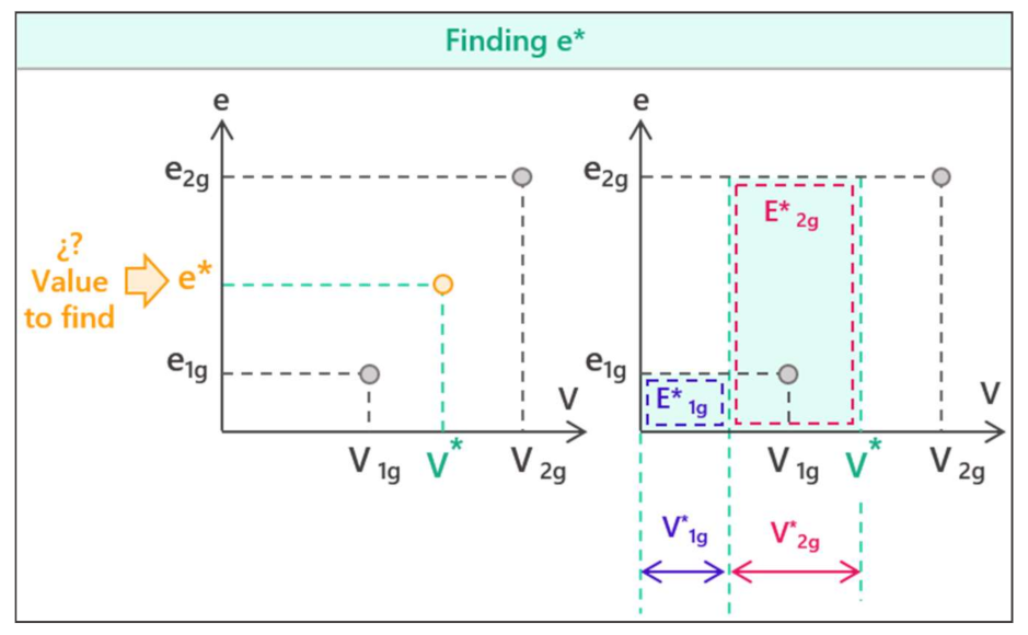
Interpretation of the analytic solution.
Equation (21) shows the analytic solution to find the average value of the specific energy e* required to pump the desired volume combining one and two groups of pumps. If instead of one and two groups of pumps, the expression is written for any group combination n
i and n
j (e.g., n
g = 1 and n
g = 3; or n
g = 2 and n
g = 3, or n
g = 2 and n
g = 4, etc.), the expression has this generic form:
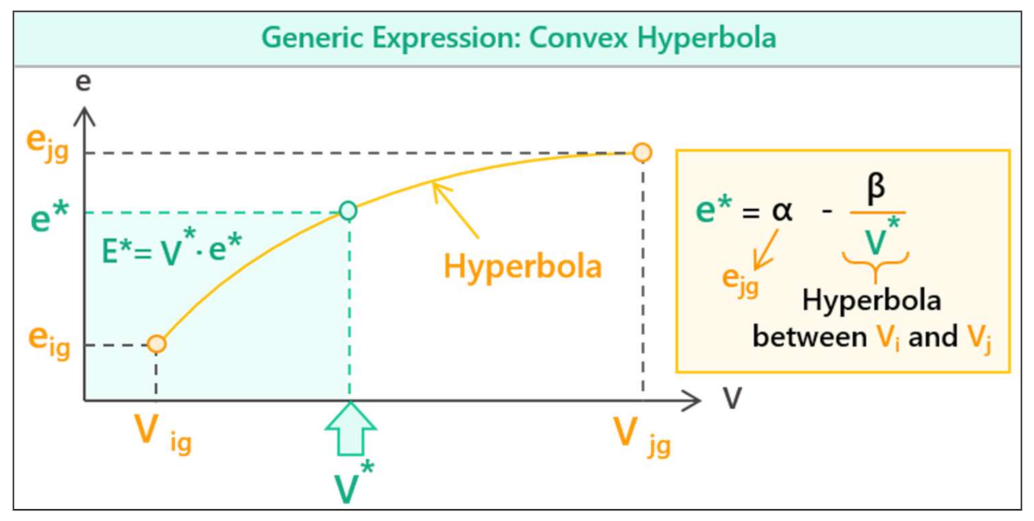
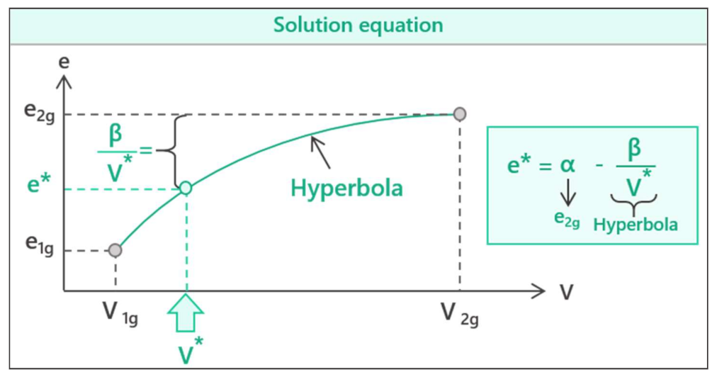
In Equation (24), all values V
ig, V
jg, e
ig, and e
jg are known, because
Table 1 is calculated in the first place. Therefore, it should be noted that this expression can be written in terms of constants in the following way:
Being:
Therefore, the most important conclusion extracted from Equation (25) is that the specific energy e* follows an inverted hyperbola shape, otherwise baptized as the Convex Hyperbola. To help visualize this conclusion,
Figure 9 is shown:
The example case that has been used for this deduction can thus be graphically represented as well, as
Figure 10 illustrates. It would be the representation of Equation (21):
It is important to notice that the combination of working groups does not have to be a consecutive number. The convex hyperbola can be graphed between any group combination ni and nj, such as. ng = 1 and ng = 3, etc. In the following section, this aspect will be covered in depth.
How to use the results: practical steps.
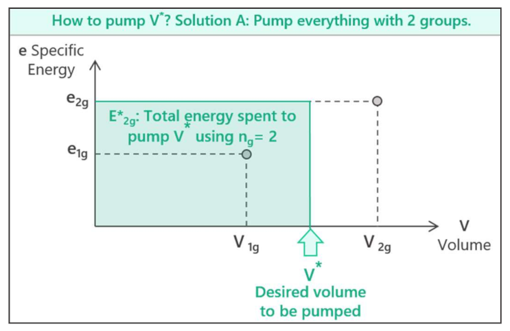
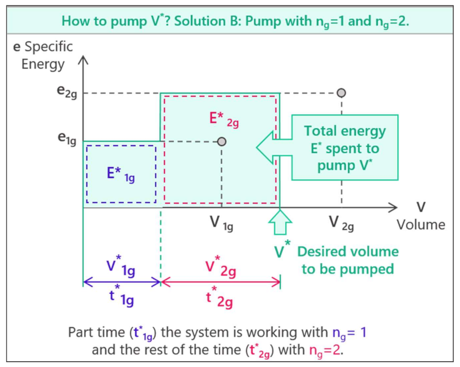
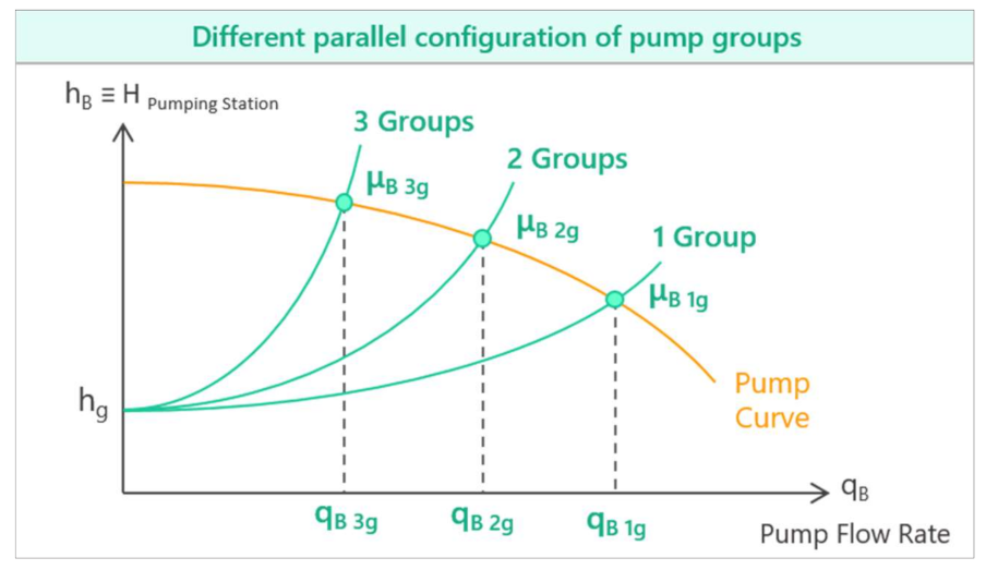
3.1. The Optimal Group Combination
In order to pump the desired water volume V*, the pumping station can be working for a portion of time with a certain amount of active groups of pumps ni, and the rest of the time with a different number of active groups nj. For instance, it could be initially one group of pumps ni = 1, and after a certain time, switch into two groups nj = 2, or instead, it could begin with three groups of pumps ni = 3, and then change to five groups of pumps nj = 5, etc.
How to choose which pump combination is the key question, and the answer is simple: the combination that consumes the least amount of energy to pump the desired volume V* should be chosen. That is to say, the combination that consumes the least specific energy e*.
3.1.1. How to Use the Results for A Certain Volume V*—Specific Case
Equation (21) demonstrates how e* can be calculated given a combination of pumps. Therefore, the strategy will consist of forming different groups of pump combinations, then calculating e* and seeing which combination works at the minimum e* for that specific V*. This process is illustrated in the following
Table 2:
Once identified the best group combination, the final step (7) would consist of using Equation (23) to find out the time each number of groups should be working.
3.1.2. How to Use the Results for Any Desired Volume V*—General Case
The previous section focuses on one specific volume V*; however, a more interesting approach is to be able to find the best combination of pumps for any desired volume V*. This can be achieved by creating a chart collection for the pumping station. In this chart, all possible volumes V* are contemplated, and it offers the best combination of pumps for any situation. To create this chart, engineers may represent the convex hyperbolas of all possible groups’ combinations of the station, using Equation (21).
The compiled steps to generate these charts are:
Step 3: Represent all the previous
Table 3 in one chart.
Step 4: Identify the curves that are the lowest. Those indicate the most convenient pump combinations for any desired volume.
Step 5: Once the best group combination is identified, use Equation (23) to find out the time each number of groups should be working.
The generation of these charts only requires a calculation sheet, and it could save a lot of energy and money by only knowing which is the least energy-using group combination to use. They do not need to be changed; on the contrary, they are a permanent guide chart for any pumping situation.
Examples
Figure 11 shows an example of a pumping station that has up to three pumps. Operators have chosen the time t
t (this could be e.g., 1, 6, 24 h, etc.). During that time, they may wish to supply different volumes of water V*. For example, if it is an hourly regulation, from 06:00–07:00, a volume of V* = 600 l might be needed, but from 07:00–08:00, they might need V* = 12.000 l. In this example, to pump any desired volume V*, operators could choose to use any of the following configurations:
One group for a while and then switch to 2 groups for the rest of the time. This is ni = 1 and then nj = 2.
One group for a while and then switch to 3 groups for the rest of the time. This is ni = 1 and then nj = 3.
Two groups for a while and then switch to 3 groups for the rest of the time. This is ni = 2 and then nj = 3.
Since there are three possible pumping configurations, three possible Convex Hyperbolas can be graphed, Equation (24). The steps to map out these hyperbolas are explained in the preceding section. Once the Convex Hyperbolas (the green lines) have been drawn (two upper figures on
Figure 11), the guidance chart for that regulation period (e.g., hourly regulation) is obtained. For each pumping station, the curves of the hyperbolas can look completely different (e.g., one hyperbola above or under the other, etc.). The curves in
Figure 11 are only an example of what they could look like.
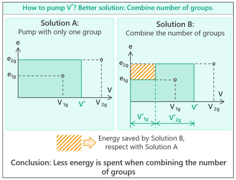
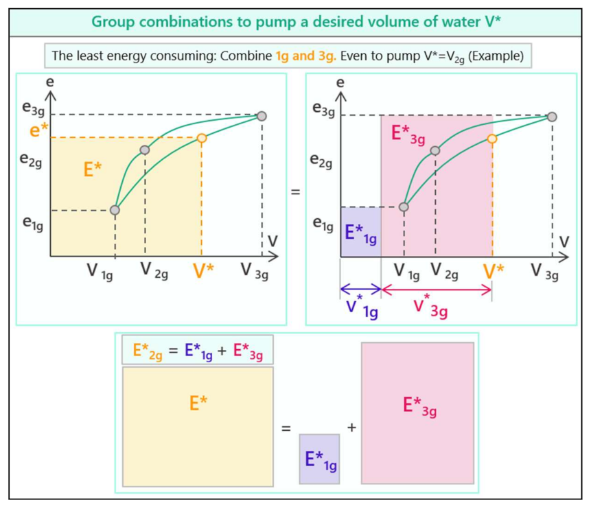
In this figure, it is represented that the best solution would be to (always) combine one group ng = 1 and three groups of pumps ng = 3 to pump any desired volume V*, since it is the lowest convex hyperbola (and therefore, the cheapest pump combination). The energy spent in this combination E* is the sum of the energy consumed while using ng = 1 (E*1g) and ng = 3 (E*3g).
One must always select the lowest Convex Hyperbola, since it indicates the least energy use. The strategy is, therefore, to always look for the lowest curve.
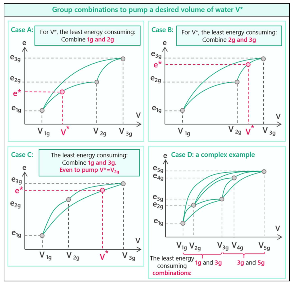
Figure 12 represents different examples of how these charts could look:
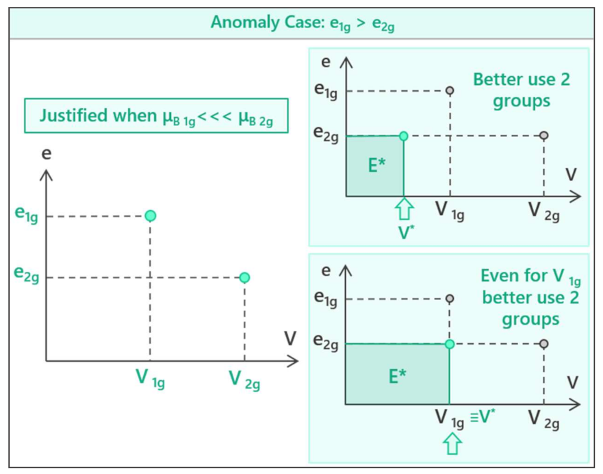
Case (a) and (b): They represent the same pumping station with three pumps. In case (a), the desired volume V*. V1g < V* < V2g would be best to pump with one and two groups. However, if the desired volume is greater, V2g < V* < V3g, the least-energy-use combination is to use two and three groups of pumps.
Case (c): The pumping station also counts with three pumps, but the convex hyperbolas show a different shape, and the least-energy-use option is to use one and three groups of pumps, for any desired volume V1g < V* < V3g.
Case (d): It illustrates a more complex situation, where the station counts for up to five pumps. In this example, the convex hyperbolas have a shape in which the lowest curves (those that show the least energy use combinations) are only the combination of one and three groups (when V1g < V* < V3g), or for bigger volumes (when V3g < V* < V5g), three and five groups.
Minimizing the vibrations in pumps by turning on and off.
It must be kept in mind that the Convex Hyperbola Charts are drawn for a defined time tt (for example 5 min, 1 h, 6 h, 24 h, etc.). During that time, operators need to provide the demanded volume of water, and the charts will indicate the best configuration (for example, firstly using 2 pumps and then switching to 4 pumps). The shorter tt (the reevaluation period), the better adjustment to variable demands. However, short reevaluation periods implicate that the pumps will be switching on and off very frequently to adjust to the demand. This is never good for the sake of the durability of the machinery, especially when the pumps are large and the vibrations can be strong. Therefore, it is always desirable to have facilities to regulate the demand at the destination point, such as tanks or reservoirs.
The present methodology requires only one change (and no more) in the configuration during each t
t (because, as it was proven in the
Section 2.2.2. Solution B, this way, the system consumes less energy). The important point is that turning on or off will only happen once during each t
t. How this one configuration change affects the durability of the pumps only depends on t
t (the reevaluation period): one configuration change in, for example, t
t = 6 h, is a minimal impact, but one configuration every t
t = 5 min, for example, can be damaging for the pumps.
However, this is external to the present method. All other optimization methods have the same restraint: every method needs to reevaluate the configuration every certain time tt. It only depends on the capability to regulate the demand, and it is always better and desirable to have some sort of deposit for this task at the destination point.
4. Discussion
This research aimed to address the number of pumps that should be working at any moment during the operation of a parallel pumping station to provide the desired volume of water whilst consuming the least amount of energy. This is not only one of the biggest environmental challenges today, but also it goes hand in hand with being economically responsible.
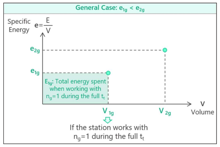
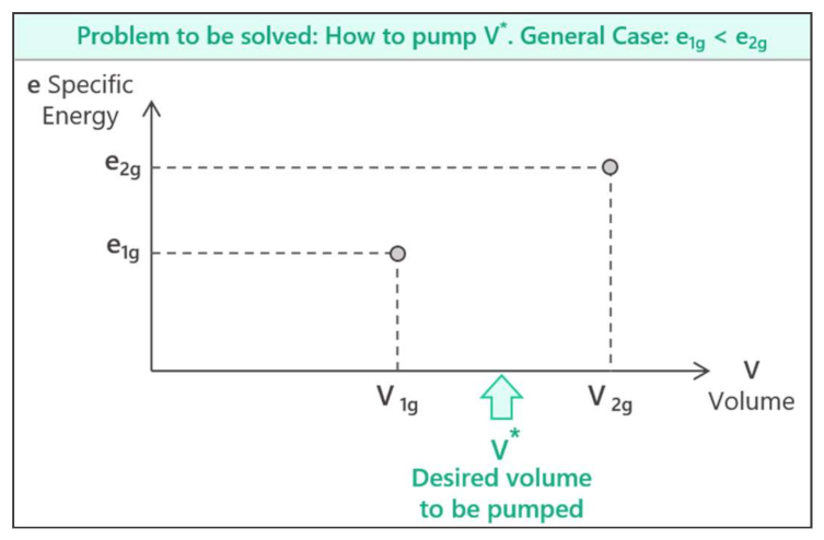
This research proposes the preparation of the Convex Hyperbolas Charts to indicate the best pumping strategy during the operation of a facility. These charts take their name from the shape of the specific energy–volume curves. The specific energy e* is the amount of energy consumed by the station per unit of volume. The pumping station should pump the desired volume of water V* using the least specific energy e*. This research analyzes the shape of the curves e*–V*. The result is that such curves have a convex hyperbola shape.
Strengths and limitations
The elaboration of the Convex Hyperbolas Charts allows engineers to know exactly what is the best number of active pumps for any pumping situation. The making of such charts only requires the use of any calculation sheet, only once, and it is a permanent resource that can be used at any time during the operation. It immediately tells the operator how many pumps should be turned on, depending on the desired volume of water. As simple as they are, these charts could save great quantities of energy and money, in both the short and the long run. The proposed methodology is completely inexpensive, in both the material and the computational aspect. It does not require any heavy complex algorithm, but on the contrary, it could be simply done with a calculation sheet. It simply comes from the mathematical deduction of the specific energy used, and not from any iterative process that is the current trend, all its applicability relying on powerful computers. Hence, the solution is not approximate, but exact. This work offers an analytic solution, which is a great advancement compared to the existing methods.
In addition, the Convex Hyperbolas Charts are completely compatible and complementary with any other operation control algorithm, and they do not need to adapt the installations or machinery. An additional advantage is that our methodology is energy cost-free: our methodology does not need to be updated with energy price changes, because it optimizes the amount of energy consumed and not its cost.
Practitioners can easily benefit from this tool thanks to its simple application: no programming or computational skills are needed. Once the charts are plotted, it is only a matter of identifying the lowest curve in the graph and selecting the indicated pump configuration. The proposed methodology is very operational-friendly. A powerful and simple tool to be more energetically mindful in the operation of water supply systems was presented.
As a limitation, it should be recalled that, just like any other optimization method, operators will need to reevaluate the pump configuration after a certain time tt, depending on the variability of the demand and the water regulation capacity. Different Convex Hyperbolas Charts will need to be elaborated for the same pumping station depending on the period considered for the optimization tt (e.g., hourly regulation, daily regulation, etc.). During the night, longer periods could be considered, whilst during the daytime, the reevaluation periods might be shorter. Nevertheless, this is a minor limitation, since it would be enough to plot a small collection of charts, according to different reevaluation periods. Additionally, all other optimization methods have the same restraint: every method needs to reevaluate the configuration every certain time. This aspect is always improved when regulation in the destination point is available (e.g., tanks, reservoirs, etc.).
Future research
One of the initial hypotheses of the method is that all pumps in the pumping station are parallel and identical. Future research will be undertaken to analyze the effects of speed controllers. The effect of the speed controller is equivalent to “changing the pumping curve”, and in this way, pumps can no longer be considered identical. This is a research line that will be studied in depth in future investigations.


