A Method for Estimating the Velocity at Which Anaerobic Metabolism Begins in Swimming Fish

Abstract

Anaerobic metabolism begins before fish reach their critical swimming speed. Anaerobic metabolism affects the swimming ability of fish, which is not conducive to their upward tracking. The initiation of anaerobic metabolism therefore provides a better predictor of flow barriers than critical swimming speed. To estimate the anaerobic element of metabolism for swimming fish, the respiratory metabolism and swimming performance of adult crucian carp (Carassius auratus, mass = 260.10 ± 7.93, body length = 19.32 ± 0.24) were tested in a closed tank at 20 ± 1 °C. The swimming behavior and rate of oxygen consumption of these carp were recorded at various swimming speeds. Results indicate (1) The critical swimming speed of the crucian carp was 0.85 ± 0.032 m/s (4.40 ± 0.16 BL/s). (2) When a power function was fitted to the data, oxygen consumption, as a function of swimming speed, was determined to be AMR = 131.24 + 461.26U_s^1.27 (R² = 0.948, p < 0.001) and the power value (1.27) of U_s indicated high swimming efficiency. (3) Increased swimming speed led to increases in the tail beat frequency. (4) Swimming costs were calculated via rate of oxygen consumption and hydrodynamic modeling. Then, the drag coefficient of the crucian carp during swimming was calibrated (0.126–0.140), and the velocity at which anaerobic metabolism was initiated was estimated (0.52 m/s), via the new method described herein. This study adds to our understanding of the metabolic patterns of fish at different swimming speeds.

1. Introduction

Construction of sluices and dams brings huge benefits in terms of flood control, irrigation and power generation, but also destroys the natural connectivity of rivers and lakes, blocking fish migration [1,2,3]. Fishways play a role in repairing this ecological damage, and successful fishways are essential for fish migration, which they assist via removing or minimizing the effects of physical barriers to movement such as a hydroelectric dams [4]. However, the flow velocity in fishways is often high, and thus they may continue to present hydraulic barriers to fish [5]. It is therefore critical to the improvement of fishway efficiency to formulate a standardized approach to the measurement of the hydraulic barrier that they present to fish.

The research focus differs depending on the stage of the fishway, and can be broadly categorized as concerning either design or operation. During the design phase, the main considerations are the hydraulic conditions within the fishway, and the control of fishway hydraulic parameters such as water velocity, intensity of turbulence, and energy dissipation rate in the pool, in order to minimize the hydraulic barriers presented to the upstream movement of fish [6,7,8,9,10]. After construction of a fishway, prototype observations can be conducted through fish release experiments to further identify flow barriers and improve the efficiency of fish passage. However, although many studies on fishway hydraulics have been conducted, the efficiency of fishways remains relatively low [11,12]. In order to improve fishway efficiency, interdisciplinary research is necessary [4]. Through study of the swimming abilities and respiratory metabolism of fish, fish biologists have divided fish swimming speeds into three categories: sustained, burst, and prolonged [13], of which the prolonged swimming speed has been measured most often in laboratory testing [14]. The main subcategory adopted has been the critical swimming speed, first defined and employed by Brett [15], which can be defined as the highest swimming speed that a fish can maintain for the time period being tested [16]. Research on respiratory metabolism is often conducted using respirometer testing [15,17], and fish energy consumption data can be obtained from measurements of their rate of oxygen consumption.

The adaptation of fish to their surrounding fluid environment can be understood from the perspective of energy consumption [18,19,20,21,22,23,24]. However, using hydrodynamic modelling to calculate swimming cost, Thiem et.al [25] did not find a difference in the rate of energy expenditure between sturgeon (Acipenser fulvescens) that were successful or unsuccessful in achieving fishway passage, even though the successful fish exhibited higher costs of transport (42.75 versus 25.85 J kg⁻¹ m⁻¹, respectively). Since energy expenditure metrics did not appear to be predictive of successful fishway passage, these researchers were led to conclude that other endogenous or exogenous factors were influencing passage success. In the drag force hydrodynamic model, it is generally assumed that the drag coefficient of a fish is identical to that of an equivalent rigid body [19,26], an assumption that may be invalid while fish are swimming. Moreover, the estimation of energy consumption via oxygen consumption does not include the energy provided by anaerobic metabolism during exercise, and many studies show that fish enter anaerobic metabolism before reaching critical swimming speed [27,28,29]. The energy contribution of anaerobic metabolism is difficult to estimate from the swimming speed of live fish.

In fishway design, the critical speed model is often quite simply applied, with fish assumed to fail passage if the water velocity within the fishway exceeds their critical swimming speed [30]. However, research results regarding respiratory metabolism have rarely been applied to fishways. Rather, hydrodynamic models have been used to calculate the drag force of fish, and estimate the energy needed to overcome this drag within the fishway. Through cross-disciplinary work combining fish biology and fish hydraulics, this paper aims to establish a relationship between respiratory metabolism and fish swimming drag force calculations. To obtain the necessary metabolic parameters in relation to swimming speed, estimating the rate of oxygen consumption for series of increasing velocities within a closed tank, which provides ample space for free swimming, has an important advantage: specifically, this avoids the reduced sensitivity to changes in oxygen levels that occur if the volume of circulating water is excessively large.

2. Materials and Methods

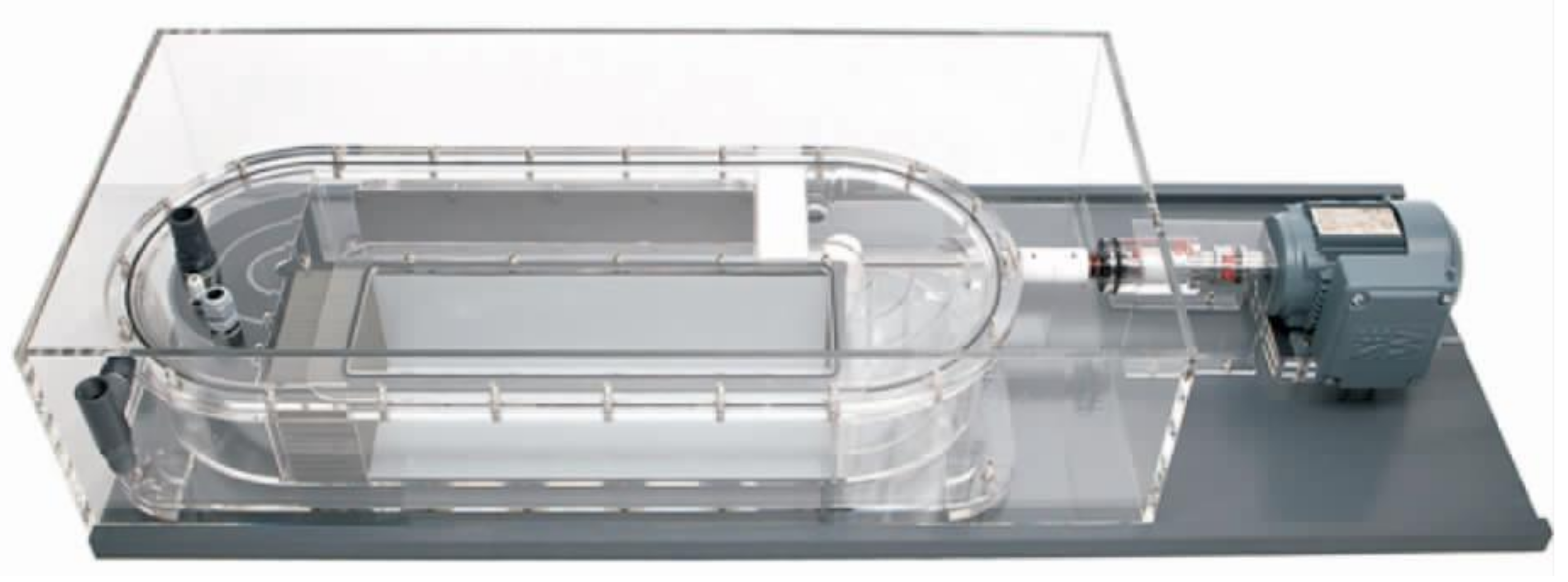
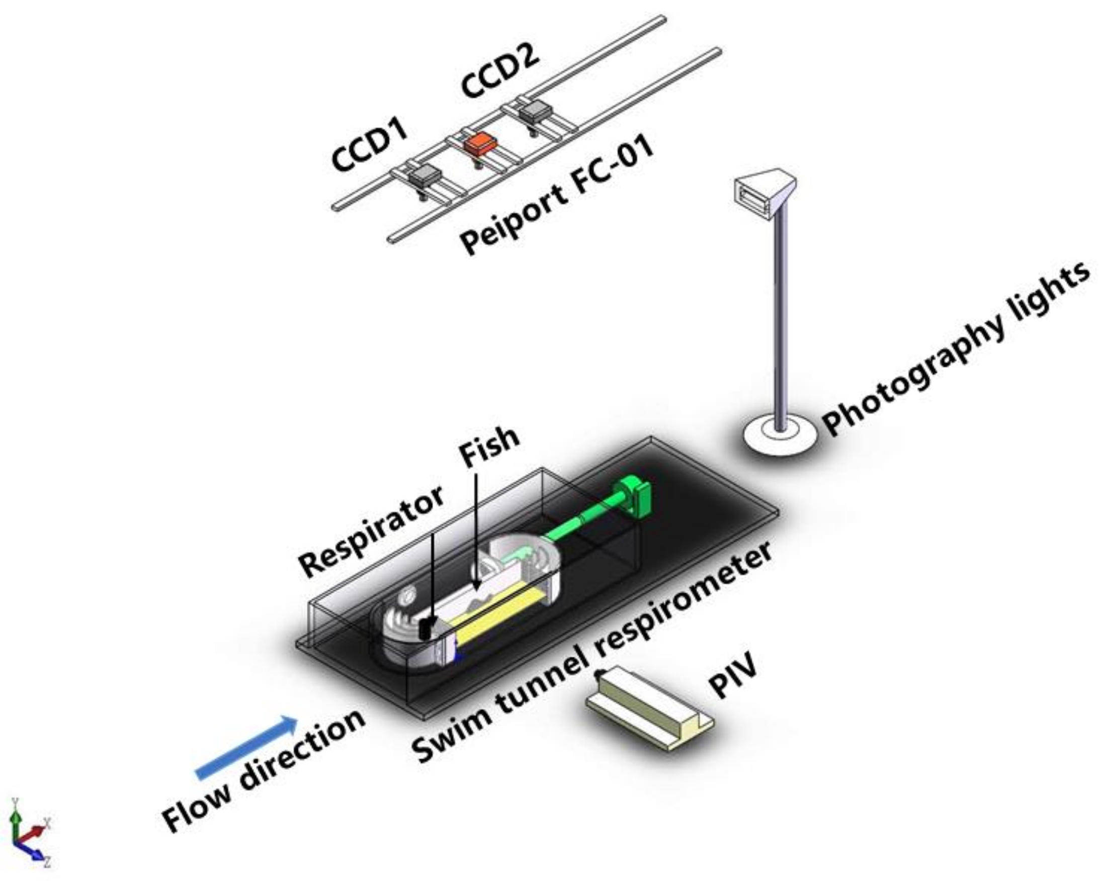
2.1. Respirometer

Fish were tested in a flume-type swimming respirometer (SW10200, Loligo Systems, Denmark), volume 90 L, with a 28 L rectangular swim chamber (0.70 m × 0.20 m × 0.20 m). The respirometer was submerged in the tank (Figure 1). The maximum water velocity possible in the chamber was 1.50 m/s. A flow rectifier maintained smooth flow within the chamber, while a grid was placed at the end of the chamber to prevent fish being swept away. Water velocity in the respirometer was controlled by a propeller driven by a variable-speed motor; this was calibrated using a LaVision Particle Image Velocimetry system (PIV). The respirometer could be flushed with a submersible pump in order to maintain the dissolved oxygen (DO) level within it. The respirometer was equipped with a high-speed video camera (Peiport FC-01, 200 HZ frame rate, 100 cm × 65 cm sampling window) set above the swim chamber to record fish swimming behavior and tail beat frequency. During the test, the respirometer was sealed, and its internal dissolved oxygen and temperature levels were monitored using a multi-parameter probe (HACH HQ30d, USA).

2.2. Experimental Design

Fish. Crucian carp (n = 31, body mass = 260.10 ± 7.93 g, total length = 24.73 ± 0.25 cm, spawning period) were obtained from a fish farm in Wuhan, Hubei, China. The fish were immediately transferred to laboratory aquaria (diameter 2.0 m, height 0.8 m), where they acclimated for at least two days. They were fed daily and any remaining food was removed after 1 hr. Testing took place from 1 July to 10 August 2019 and was carried out in the Key Laboratory of Ecological Impacts of Hydraulic-Projects and Restoration of Aquatic Ecosystem of the Ministry of Water Resource, Wuhan, China, with room temperature controlled by air conditioning. The test fish were kept temporarily in the pool on site for 2 d and not fed for the 24 h period prior to being transferred, in water, to the respirometer [15]. The duration of each test was around 6 h. Dissolved oxygen (DO) within the respirometer was maintained above 6.0 mg/L [29], and the water temperature maintained at 20(±1) °C. When the DO fell below 6.0 mg/L, testing was interrupted and the water was aerated [17]. Sample numbers and corresponding water velocities are shown in

Table 1. Number of samples at each stage. When the velocity (m/s) reaches the critical swimming speed, the number of samples naturally decreases.

Number of Samples	0.15 (m/s)	0.30 (m/s)	0.45 (m/s)	0.60 (m/s)	0.75 (m/s)	0.90 (m/s)	1.05 (m/s)	1.20 (m/s)
n	31	31	31	31	25	14	7	2

.

Cameras. The PIV laser was placed horizontally emitting a light surface parallel to the bottom surface of the device, in order to ensure that the two horizontally-oriented CCD cameras could photograph the test plane illuminated by the laser; the details were described in Tarrade’s paper [31]. The high-speed video camera was set above the chamber to record the swimming behavior of the fish (video was recorded during the test and the tail beat frequency could be obtained through frame-by-frame analysis by ProAnaly software). It was ensured that the three cameras were capturing the same plane. The requisite supplementary light sources were also set up alongside the test device (Figure 2).

Calibration. The relationship between the frequency setting of the variable-speed motor, x, and water velocity, y, was calibrated using the LaVision Particle Image Velocimetry system (PIV). The equation y = 0.03788x (R² = 0.9978) fitted this data. (See Appendix A.) During testing, the rotation speed of the motor was adjusted using its frequency setting, in order to control the water velocity in the swim chamber.

Stepped Velocity Testing. Stepped velocity tests were conducted to estimate the critical swimming speed (U_crit), oxygen consumption rate (AMR), cost of transport (COT), and tail beat frequency (TBF) of the crucian carp; these tests were repeated n times (Table 1). During each test, water velocity was increased by 0.15 m/s, starting at 0.15 m/s, at 25-min intervals until the test fish was fatigued. At the same time, the DO (mg/L) and temperature in the respirometer were recorded every 5 min for 25 min. A fish was considered as fatigued when it stopped at the end of the test area, lightly patted the downstream wall for 20 s and still could not swim [32]. After testing was complete, the body length (cm), total length (cm), and body mass (g) of the fish were measured.

2.3. Morphometric and Statistical Analysis

The critical swimming speed U_crit was calculated using the flow velocities and step intervals recorded during the test using Equation (1) [14]:

$$U_{crit}=v+\frac{t}{∆t}∆v$$

(1)

where t (min) is the time elapsed at fatigue velocity, Δt (min) is the prescribed interval time (here 25 min). Δv (m/s) is the velocity increment (here 0.15 m/s), and v (m/s) is the final velocity recorded before the fish became fatigued. It was ensured that the cross-sectional area of the test fish was less than 10% of the cross-sectional area of the test area. This prevented it causing a blocking effect, and eliminated the need for a correction in Equation (1) [33].

Oxygen consumed per hour per kilogram of body mass (AMR) was obtained using Equation (2) [34]:

$$AMR=\left(St-Sb\right)\times 60\times Vol/m$$

(2)

where AMR is the oxygen consumption rate of the standard weight of the test fish (mg O₂·h⁻¹·kg⁻¹); St is the value of the slope of dissolved oxygen with respect to time with the test fish swimming (apparent oxygen consumption mg O₂·min⁻¹·L⁻¹); Sb is the absolute value of the slope of dissolved oxygen per unit time in the absence of a test fish (bacterial oxygen consumption mg O₂·min⁻¹·L⁻¹); 60 is the time constant (s/min); Vol is the total volume (L) of the experimental water system (90 L in this study), and m is the body mass of the fish (kg).

The cost of transport (COT) (J·kg⁻¹·m⁻¹) is the energy expended in swimming, which was obtained using Equation (3) [25]:

$$COT=\frac{AMR}{U_s}\times 13.54$$

(3)

where U_s is swimming speed (m·s⁻¹) and 13.54 is the oxycaloric value (J·mg O₂⁻¹) [35].

Vogel [26] proposed that the drag of a fish moving through water can be determined using Equation (4) [21,24]:

$$F=0.5C_d\rho A_s{U}_s{}^2$$

(4)

where C_d is the drag coefficient; ρ is the density of water (1000 kg·m⁻³); A_s is the wetted surface area of the fish, which can be calculated using Equation (5); and U_s is the swimming speed. C_d is composed of two factors, the frictional drag coefficient C_f and pressure drag coefficient C_p. C_d can be obtained using Equations (6)–(8) [19,20]:

$$A_s=\alpha L^{\beta }$$

(5)

$$C_d=C_f+C_p\approx 1.2C_f$$

(6)

$$C_f=0.074R{e}^{-0.2}$$

(7)

$$C_d=0.088R{e}^{-0.2}$$

(8)

where Re is the Reynolds number, Re = LU_s/ѵ [33] (ѵ is the kinematic viscosity of water); α and β are empirical constants, α = 0.465, β = 2.11 [20]; and L is the body length of the fish.

The metabolic rate of the fish was modelled as being divided into aerobic and anaerobic metabolism. Since the only variable in the test is swimming speed, the total mechanical power caused by differences in speed can be obtained from Equation (9):

$$P_s=\left(AMR-AM{R}_0\right)\times m\times 13.54/3600$$

(9)

where AMR₀ (mg O₂·h⁻¹·kg⁻¹) is the oxygen consumed per hour per kilogram of body mass in still water.

The drag on the fish is F and thus the mechanical power needed to overcome the drag is FU_s. The energy efficiency of fish swimming under aerobic metabolism can be obtained using Equation (10) [36]:

$$\eta =\frac{P_d}{P_s}\times 100\%$$

(10)

where the P_d (W) is the power of the drag, P_d = FU_s.

2.4. Data Analysis

Linear regression analysis, calculated with Origin 8.5 statistical software, was applied. The drag and the energy efficiency data are expressed as means; other data (body length, total length, body mass, critical swimming speed, oxygen consumption rate, cost of transport, tail beat frequency) are expressed as means ± standard errors (mean ± SEM). The error bars in the figures below represent standard errors. The significance level for F-tests was set as p < 0.001.

3. Results

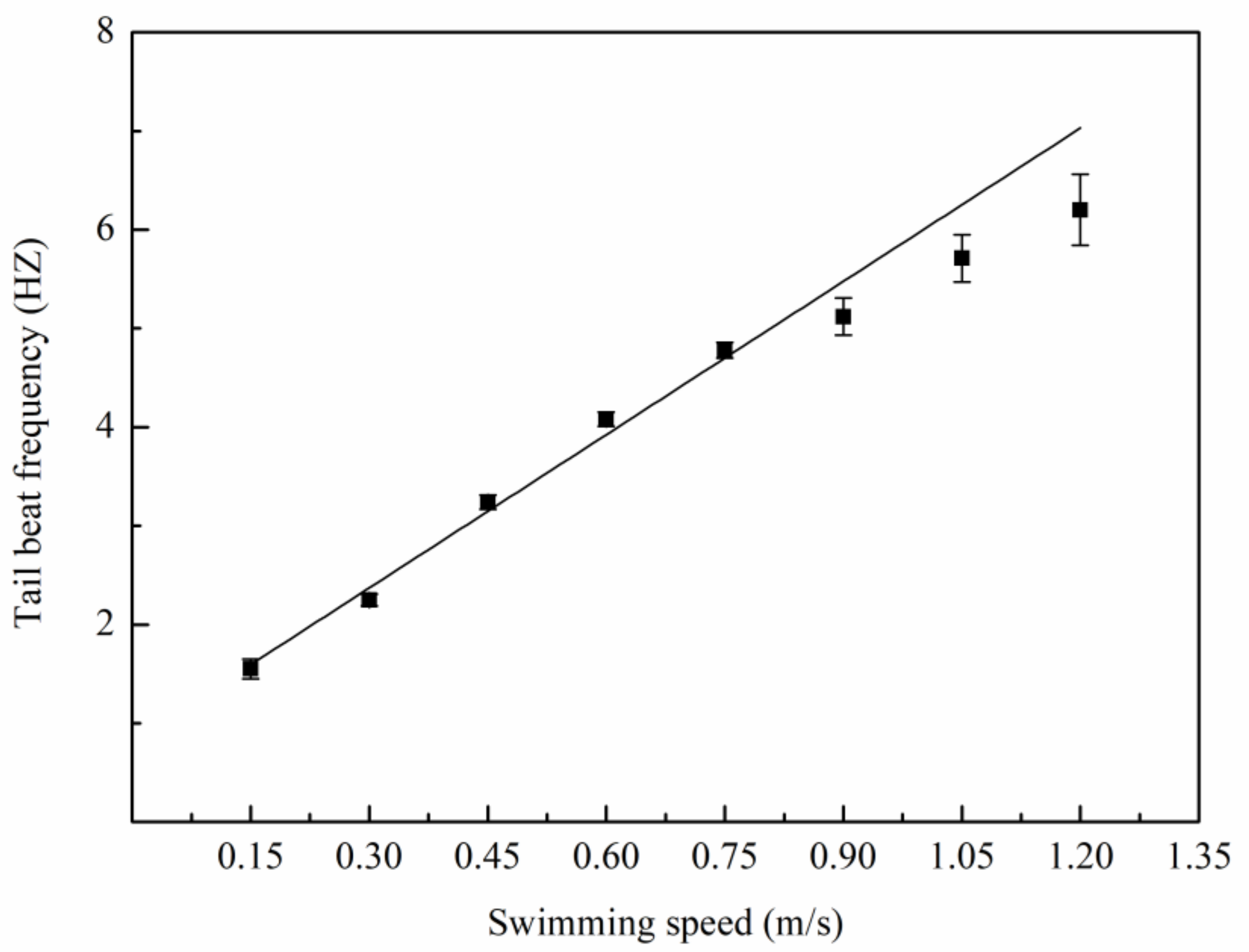
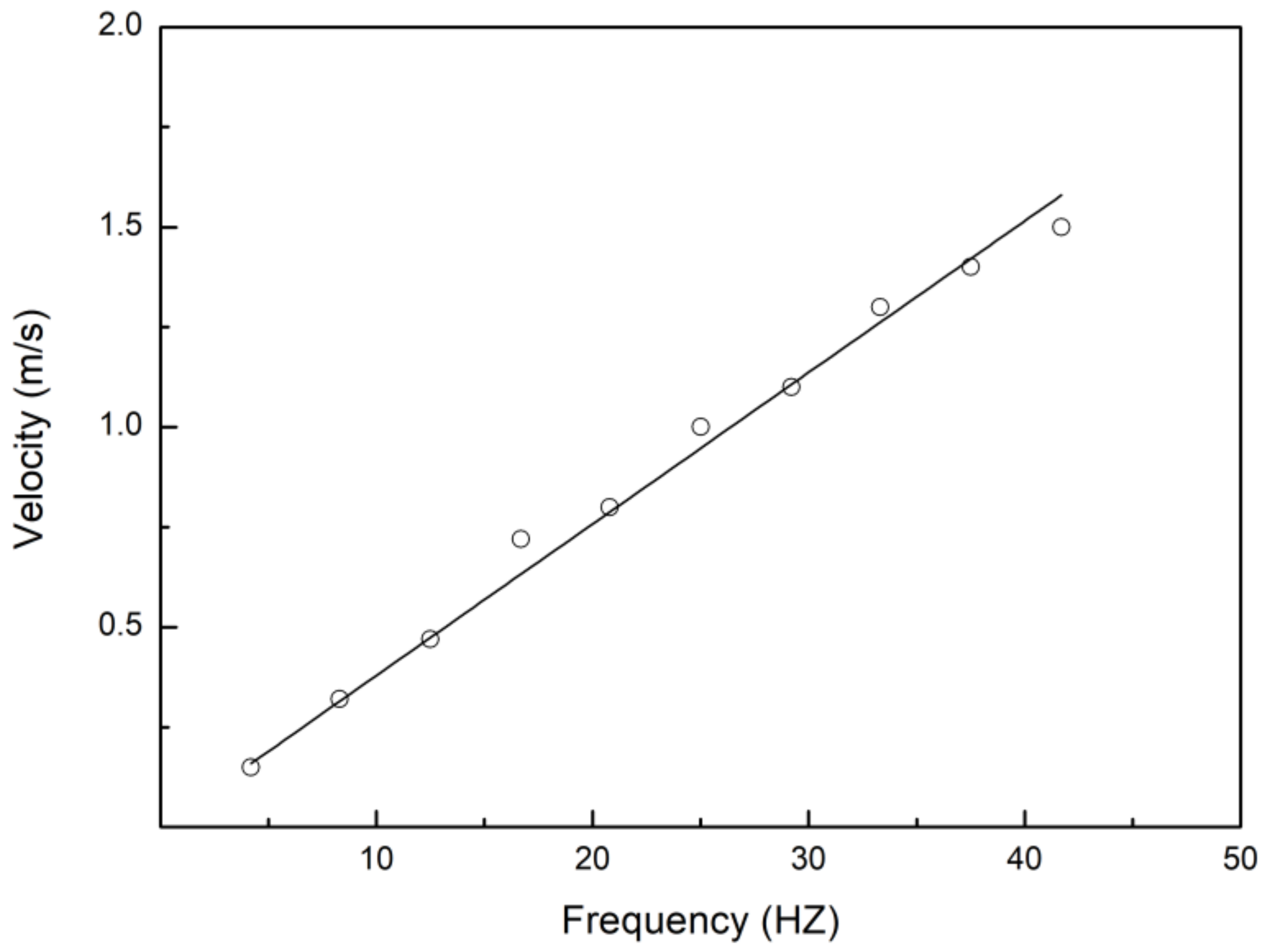
3.1. Swimming Kinematics

The crucian carp tested under 20 ± 1 °C water temperature conditions had a total length of 24.73 ± 0.25 cm, body length of 19.32 ± 0.24 cm, and body mass of 260.10 ± 7.93 g. Their U_crit was 0.85 ± 0.032 m/s (4.40 ± 0.16 body lengths, BL/s). Correlation between swimming speed U_s and tail beat frequency TBF are shown in Figure 3. The equation TBF = 0.82 + 5.2 U_s (R² = 0.977, p < 0.001) was fitted to this data. For the highest water velocities, in excess of U_crit, the fit was poorer than for lower velocities.

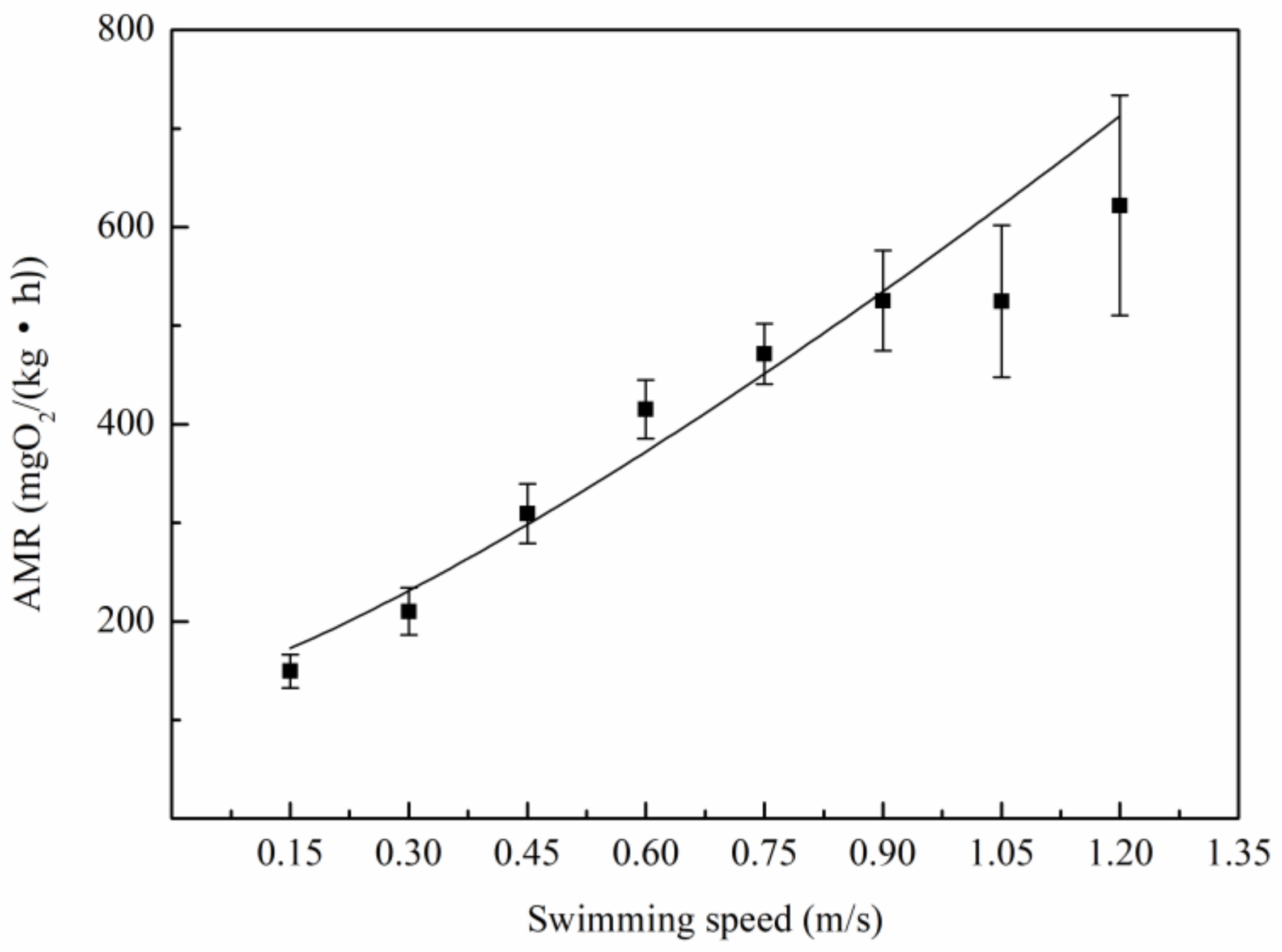
3.2. Relationship Between Oxygen Consumption and Water Velocity

The relationship between rate of oxygen consumption and swimming speed (Figure 4) was estimated using Equation (2), AMR = 131.24 + 461.26 U_s^1.27 (R² = 0.948, p < 0.001). For the highest water velocities, in excess of U_crit, the fit was poorer than for lower velocities. The rate of oxygen consumption in still water was 131.24 ± 13.44 mg O₂·h⁻¹·kg⁻¹. As water velocity increased, the rate of oxygen consumption also increased, varying over velocity intervals. However, the rate of increase varied over velocity intervals. With water velocity at 1.2 m/s, the rate of oxygen consumption reached its maximum, at 621.92 ± 111.74 mg O₂·h⁻¹·kg⁻¹.

The relationship between COT and swimming speed, U_s, is shown in Figure 5. Based on the relationship between COT and AMR, the relationship between COT and U_s was calculated using Equation (3), as COT = 0.49 U_s⁻¹ + 1.73 U_s^0.27 (R² = 0.594, p < 0.001).

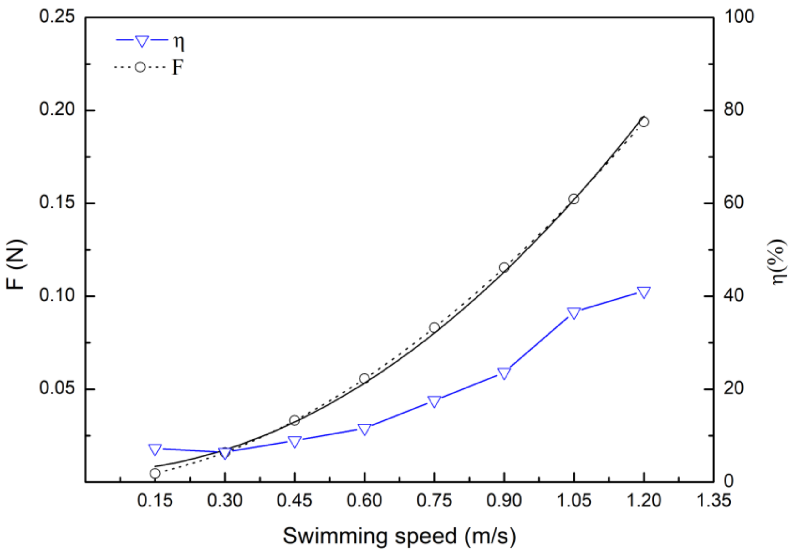
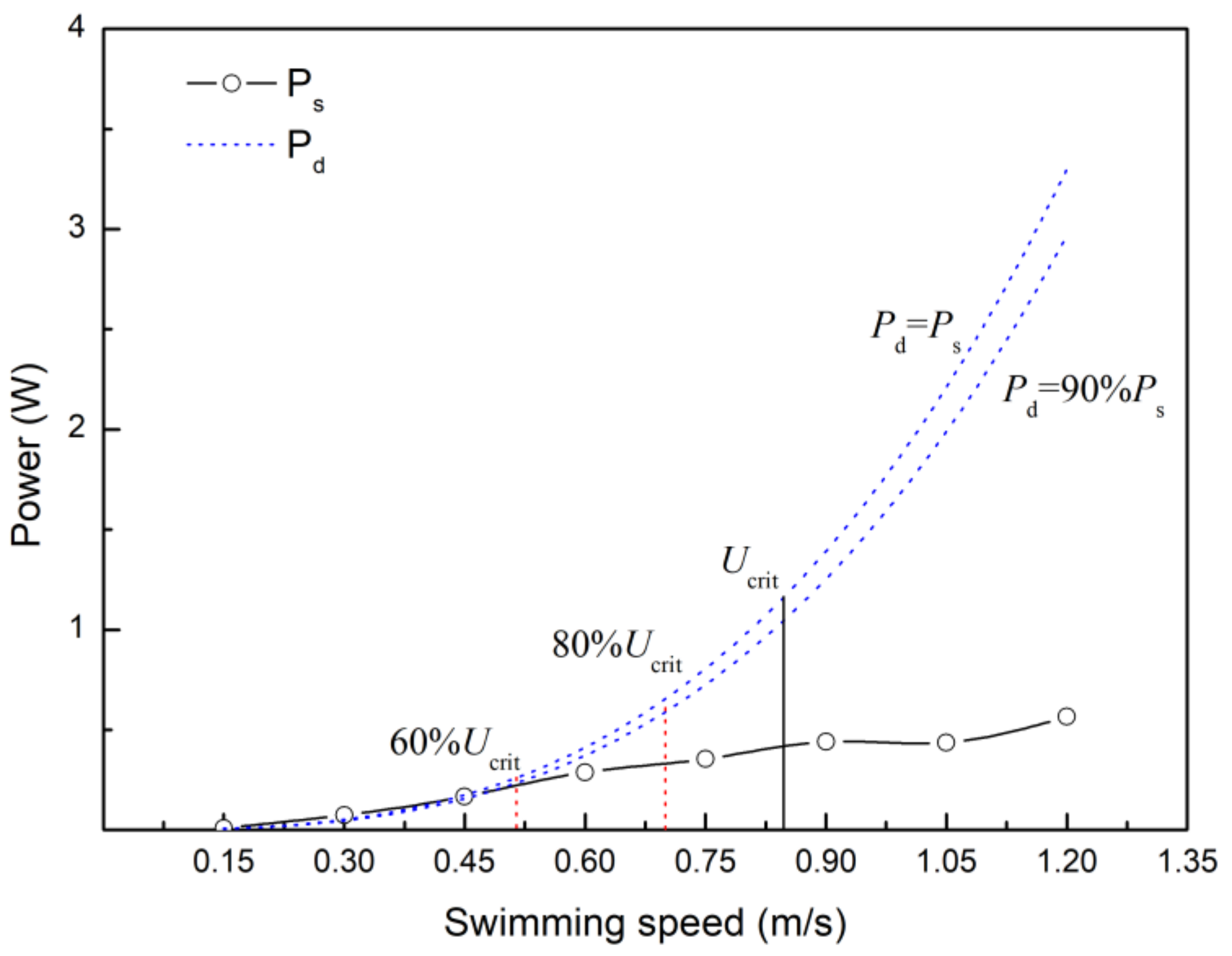
3.3. Drag Calculation Based on Hydrodynamic and Energy Efficiency

The relationship between drag and swimming speed is shown in Figure 6. As the speed of the water increases, drag increases, with data fitting the equation F = 0.0055 + 0.13 Us (R² = 0.998, p < 0.001).

Based on Equations (4)–(10), the estimated relationship between crucian carp energy efficiency and swimming speed is as shown in Figure 6. Energy efficiency increased with swimming speed, over the range 7.25–41.13%.

4. Discussion

Hydraulic factors in the fishway, such as water velocity, energy and intensity of turbulence, unit volume dissipation rate and strain rate, are important determinants of whether fish successfully migrate upstream [37,38]. Fish metabolism is also affected by many ecological factors [39,40]. Stimulation caused by changing hydraulic factors in fish courses will often lead to fish exhibiting behavioral responses, and these behavioral changes can cause significant metabolic changes, which in turn cause changes in energy requirements [41].

4.1. Swimming Kinematics

Critical swimming speed U_crit is an important parameter used in fishway design [42]. The U_crit is related to the duration and speed increments used during testing [34]. In this study, with water temperature at 21 ± 1 °C, 25 min duration stages, and 0.15 m/s speed increments, the critical speed for crucian carp of body length 19.32 ± 0.24 cm was 0.85 ± 0.032 m/s (4.40 ± 0.16 BL/s). The critical swimming speed of crucian carp determined by Li et al. [43] was 1.19 ± 0.024 m/s (5.91 ± 0.09 BL/s, with body length of 20.0 ± 0.80 cm). The fish used in both this and Li’s study were crucian carp of similar body length, but their source, habitat/environment and living habits were quite different. The crucian carp used in this study came from a fishing ground in the Wuhan area; those used in Li′s study came from a fishing ground in the Harbin area, and had higher critical swimming speeds.

At a stable swimming speed, fish use their bodies and tail fins to generate a propulsive force to further increase swimming speed. Previous studies [17,32,44,45] have found that the tail beat frequency of many bony fish species positively correlated with swimming speed, and a similar trend relationship was obtained for crucian carp in this study (Figure 3). The deviation from the linear relationship and increased standard deviation apparent at higher velocities may be related to the significantly reduced sample sizes available at those velocities (Table 1).

4.2. The Relation Between Metabolic Rate and Speed

The relationship between the oxygen consumption rate of fish and their swimming speed is often fitted using relationships with four functional forms [46,47,48]: linear, exponential, logarithmic and power functions. In the hydraulic model, the mechanical energy required to overcome the drag force of a swimming fish is a power function of its velocity. In addition, a review of related literature indicated that the power function model was the most commonly used, and so this was adopted for fitting in this study. In the power function model, AMR = a + b U_s^c, the velocity index, c, is typically in the range 1.1–3.3 [49]. In this study, the velocity index for the crucian carp was 1.27, reflecting their energy efficiency during aerobic exercise. (The higher the index, the lower the swimming energy efficiency, and vice versa.) In Beamish’s [50] research on the velocity indexes of several bony fish species, their mean value was 2.3. The smaller speed index determined in this study indicates a higher energy efficiency.

The energy cost per unit distance, COT, is a reflection of the energy efficiency of the exercise process as a whole; the lower its value, the higher the energy efficiency. In this study, the energy cost per unit distance of crucian carp showed a tendency to decrease with increasing swimming speed because of the gradually decreasing contribution of basal metabolism to the total oxygen consumption rate [51]. This result is similar to that of Cai et al. [17].

If the metabolic mode during exercise is purely aerobic, then total energy consumption can be calculated using the rate of oxygen consumption measured during testing. But many studies [29,52,53] have shown that anaerobic metabolism begins while fish are swimming below the critical swimming speed. As a result, energy consumption calculated based upon oxygen consumption will tend to underestimate total energy consumption. However, the mechanical energy necessary for fish to overcome drag can be calculated using hydrodynamic models. The energy provided by anaerobic metabolism can then be obtained by subtracting a measure of energy consumption based on aerobic metabolism from the estimated mechanical energy required to overcome drag.

4.3. Drag Coefficient and Drag Force

At higher Re numbers the dynamic forces of the fluid gain importance, and bodies moving through fluids must be streamlined to reduce drag [51]. The drag force on a steadily moving fish can be calculated using the hydrodynamic model, F = 0.5 C_d ρ A_s U_s. At low values of Re, A_s is usually based on frontal area whereas at higher values of Re, total wetted area is commonly used [51]. In this test, with 3476 < R_e < 59583, the decision was taken to use total wetted area, calculated using Equation (5), which was formulated to describe the wetted area of a salmonid [33]. The drag coefficient C_d is a complicated function of the Re number and its value depends on the flow conditions surrounding a body [33]. Under turbulent conditions, C_d gradually decreases as Re increases, approximately in proportion with Re^−0.2.

Using drag forces at various speeds calculated according to the hydrodynamic model, the estimated maximum energy efficiency, η, of the fish was only 41.13% (Figure 6). This is inconsistent with the observed energy efficiency of fish in nature, which exceeds 90% [36], implying that either the wetted surface area, A_s, or the drag coefficient, C_d, used in the calculation was too small, resulting in excessively low energy efficiency η. However, the incorrectness of A_s was excluded by using the measured surface area of the fish.

According to the law of conservation of energy, calibration of C_d was then possible. The calibration principle follows the boundary layer separation theory of hydraulics under high Reynolds number values, i.e., for 103 < Re < 2 × 105, C_d can be regarded as a constant, the position of the separation point remains basically constant, and F∝ U_∞² [54]. With the swimming attitude at different water velocities remaining basically unchanged, along with the angle of attack, the drag coefficient C_d can be treated as a constant. For the range of Re numbers mentioned above, drag F will be proportional to U_s², and the power needed to overcome this drag will therefore be proportional to U_s³. During exercise entailing purely aerobic respiration, it can be assumed that η = 90%−100% (P_s = 0.9−1.0 P_d), and fitting of the relationship between P_s and U_s should assume proportionality to the third power of the latter; that is, P_d = k U_s³ = 90%P_s and P_d = k U_s³ = 100%P_s (k is a constant). According to Equations (4) and (10), a formula for C_d can then be derived via inversion: C_d = 2k/ρA_s.

Studies have demonstrated that the energy efficiency of fish increases rapidly until around 70% of the critical swimming speed has been achieved [29,52,53], and that anaerobic metabolism starts at approximately 80% of the critical swimming speed [28,29]. Therefore, we assumed that while water velocity remained below 0.45 m/s (less than 60% U_crit) during testing, fish were relying purely upon aerobic respiration, and the oxygen consumption rate could be used to estimate the total energy consumption of fish at these swimming speeds. Power for low-flow aerobic swimming was then fitted (Figure 7) resulting in the equations P_s = 1.718 U_s³ (P_s = 0.9 P_d, R² = 0.953, p < 0.001), and P_s = 1.910 U_s³ (P_s = 1.0 P_d, R² = 0.954, p < 0.001); that is, k = 1.718–1.910. From this, the drag coefficient, C_d = 0.126–0.140 can be derived, with a value larger than the estimate obtained using Equation (8) (

Table 2. Drag coefficients at various water velocities.

Drag Coefficients	0.15 m/s	0.30 m/s	0.45 m/s	0.60 m/s	0.75 m/s	0.90 m/s	1.05 m/s	1.20 m/s
Cd	0.0149	0.0130	0.0120	0.0113	0.0108	0.0104	0.0101	0.0098
Calibration	Cd = 0.126–0.140

), but smaller than the drag coefficient (0.45) [54] for flow past a round sphere at the corresponding Reynolds number. Considering that the bodies of fish are streamlined, it is reasonable that their drag coefficients are smaller than that of a sphere.

4.4. Estimating the Velocity at which Anaerobic Metabolism Begins

After correcting the drag coefficient, the drag power of the crucian carp was compared with the aerobic power (Figure 7). It was found that the drag power, P_d, of the crucian carp began to exceed their aerobic power, P_s, at a water velocity of 0.52 m/s. Since drag power exceeding aerobic power likely indicates the initiation of anaerobic metabolism, the swimming speed corresponding to the point of divergence between P_d and P_s can be viewed as the velocity at which anaerobic metabolism is initiated, and the excess of P_d over P_s as an estimate of non-aerobic cost. As water velocity increased to 0.90 m/s, the power provided by aerobic metabolism reached a maximum from which it scarcely increased further. However, as water velocity increased, more power was needed, and the non-aerobic cost continued to increase. This non-aerobic cost is unfavorable to the upstream migration of fish, so, during the design of fishways, it is very important to obtain well-founded estimates of the water velocity at which anaerobic metabolism begins [53], despite the difficulty of this task [29].

In this study, by comparing the drag power and aerobic power of the crucian carp, a method of estimating the velocity at which anaerobic metabolism begins was proposed. An approximate estimate of the carp initial velocity under 20 ± 1 °C water temperature conditions for anaerobic metabolism of 0.52 m/s was obtained, a finding consistent with the observation that excess post-exercise oxygen costs begin to be observed in the range 60–80% U_crit [28]. This value may be different for different temperatures, species and environments. In this study, for crucian carp swimming at 60% U_crit (0.51 m/s), drag power, P_d, was almost equal to the capacity of aerobic respiration to generate energy for swimming (P_d = 90%P_s); for crucian carp swimming at 80% U_crit, P_d was almost two times P_s; for carp swimming at U_crit, P_d was almost 2.5 times P_s. However, as swimming speed surpassed U_crit, sample sizes were significantly reduced, and the quality of these estimates inevitably deteriorated. Anaerobic costs become necessary when fish swim at high speeds, and when these exceed a certain limit, may result in irreversible damage to their health [29]. Further research is necessary to determine the maximum speeds at which fish can swim without incurring irreversible health damage.

5. Conclusions

Measurement results for the metabolic rates of crucian carp swimming at various speeds were obtained. A method for estimating the velocity at which anaerobic metabolism begins was proposed. A flaw of this method lies in the requirement for an assumption regarding the energy efficiency of the test fish (i.e., that it lies in the range 0.90–1.0) for calibration of the drag coefficient C_d, since the excess post-exercise oxygen consumption at high speed is not measured. A pressing need for accurate measurements of the energy efficiency and excess post-exercise oxygen consumption of a wide range of fish species remains.

References

1. Mao, X. Review of fishway research in China. Ecol. Eng. 2018, 115, 91–95. [Google Scholar] [CrossRef]
2. Cooke, S.J.; Cech, J.J.; Glassman, D.M.; Simard, J.; Louttit, S.; Lennox, R.J.; Cruz-Font, L.; O’Connor, C.M. Water resource development and sturgeon (Acipenseridae): State of the science and research gaps related to fish passage, entrainment, impingement and behavioural guidance. Rev. Fish Biol. Fish. 2020, 30, 219–244. [Google Scholar] [CrossRef]
3. Fuentes-Perez, J.F.; Silva, A.T.; Tuhtan, J.A.; Garcia-Vega, A.; Carbonell-Baeza, R.; Musall, M.; Kruusmaa, M. 3D modelling of non-uniform and turbulent flow in vertical slot fishways. Environ. Model. Softw. 2018, 99, 156–169. [Google Scholar] [CrossRef]
4. Silva, A.T.; Lucas, M.C.; Castro-Santos, T.; Katopodis, C.; Baumgartner, L.J.; Thiem, J.D.; Aarestrup, K.; Pompeu, P.S.; O’Brien, G.C.; Braun, D.C.; et al. The future of fish passage science, engineering, and practice. Fish Fish. 2018, 19, 340–362. [Google Scholar] [CrossRef] [Green Version]
5. Grossman, G.; Ratajczak, R.; Farr, M.D.; Wagner, C.M. Why there are fewer fish upstream. Am. Fish. Soc. Symp. 2010, 73, 63–81. [Google Scholar]
6. Rodríguez, T.T.; Agudo, J.P.; Mosquera, L.P. Evaluating vertical-slot fishway designs in terms of fish swimming capabilities. Ecol. Eng. 2006, 27, 37–48. [Google Scholar] [CrossRef]
7. Wu, S.; Rajaratnam, N.; Katopodis, C. Structure of flow in vertical slot fishway. J. Hydraul. Eng. 1999, 125, 351–360. [Google Scholar] [CrossRef]
8. Ballu, A.; Pineau, G.; Calluaud, D.; David, L. Experimental-Based Methodology to Improve the Design of Vertical Slot Fishways. J. Hydraul. Eng. 2019, 145, 04019031.1–04019031.10. [Google Scholar] [CrossRef]
9. Li, Y.; Wang, X.; Xuan, G.; Liang, D. Effect of parameters of pool geometry on flow characteristics in low slope vertical slot fishways. J. Hydraul. Res. 2019, 1–13. [Google Scholar] [CrossRef]
10. Larinier, M.; Travade, F.; Porcher, J.P. Fishways: Biological bais, design criteria and monitoring. Bull. Fr. Pêche Piscic 2002, 9–20. [Google Scholar] [CrossRef]
11. Calles, O.; Greenberg, L. Connectivity is a two-way street-the need for a holistic approach to fish passage problems in regulated rivers. River Res. Appl. 2009, 25, 1268–1286. [Google Scholar] [CrossRef]
12. Ovidio, M.; Sonny, D.; Watthez, Q.; Goffaux, D.; Detrait, O.; Orban, P.; Nzau Matondo, B.; Renardy, S.; Dierckx, A.; Benitez, J.-P. Evaluation of the performance of successive multispecies improved fishways to reconnect a rehabilitated river. Wetl. Ecol. Manag. 2020. [Google Scholar] [CrossRef]
13. Santos, H.D.E.; Viana, E.; Pompeu, P.S.; Martinez, C.B.J.N.I. Optimal swim speeds by respirometer: An analysis of three neotropical species. Neotrop. Ichthyol. 2012, 10, 805–811. [Google Scholar] [CrossRef]
14. Plaut, I. Critical swimming speed: Its ecological relevance. Comp. Biochem. Physiol. Part A Mol. Integr. Physiol. 2001, 131, 41–50. [Google Scholar] [CrossRef]
15. Brett, J.R. The Respiratory Metabolism and Swimming Performance of Young Sockeye Salmon. J. Fish. Res. Board Can. 1964, 21. [Google Scholar] [CrossRef]
16. Peake, S. An Evaluation of the Use of Critical Swimming Speed for Determination of Culvert Water Velocity Criteria for Smallmouth Bass. Trans. Am. Fish. Soc. 2004, 133. [Google Scholar] [CrossRef]
17. Cai, L.; Taupier, R.; Johnson, D.; Tu, Z.; Liu, G.; Huang, Y. Swimming Capability and Swimming Behavior of Juvenile Acipenser schrenckii. J. Exp. Zool. Part A Ecol. Genet. Physiol. 2013, 319A, 149–155. [Google Scholar] [CrossRef] [PubMed]
18. Pedley, T.J.; Hill, S.J. Large-amplitude undulatory fish swimming: Fluid mechanics coupled to internal mechanics. J. Exp. Biol. 1999, 202, 3431–3438. [Google Scholar] [CrossRef] [PubMed]
19. Haefner, J.W.; Bowen, M.D. Physical-based model of fish movement in fish extraction facilities. Ecol. Model. 2002, 152, 227–245. [Google Scholar] [CrossRef]
20. Gu, K.-H.; Chang, K.-H.; Chang, T.-J. Numerical Investigation on Three-Dimensional Fishway Hydrodynamics and Fish Passage Energetics. J. Taiwan Agric. Eng. 2007, 54, 64–84. [Google Scholar]
21. Khan, L.A. A three-dimensional computational fluid dynamics (CFD) model analysis of free surface hydrodynamics and fish passage energetics in a vertical-slot fishway. N. Am. J. Fish. Manag. 2006, 26, 255–267. [Google Scholar] [CrossRef]
22. Standen, E.M.; Hinch, S.G.; Healey, M.C.; Farrell, A.P. Energetic costs of migration through the Fraser River Canyon, British Columbia, in adult pink (Oncorhynchus gorbuscha) and sockeye (Oncorhynchus nerka) salmon as assessed by EMG telemetry. Can. J. Fish. Aquat. Sci. 2002, 59, 1809–1818. [Google Scholar] [CrossRef]
23. Wolfgang, M.J.; Grosenbaugh, M.A. Near-body flow dynamics in swimming fish. J. Exp. Biol. 1999, 17, 202. [Google Scholar]
24. Pettersson, L.B.; BroÈnmark, C. Energetic Consequences of an Inducible Morphological Defence in Crucian Carp. Oecologia 1999, 121, 12–18. [Google Scholar] [CrossRef]
25. Thiem, J.D.; Dawson, J.W.; Hatin, D.; Danylchuk, A.J.; Dumont, P.; Gleiss, A.C.; Wilson, R.P.; Cooke, S.J. Swimming activity and energetic costs of adult lake sturgeon during fishway passage. J. Exp. Biol. 2016, 219, 2534–2544. [Google Scholar] [CrossRef] [PubMed] [Green Version]
26. Vogel, S. Life in Moving Fluids; Priceton University Press: Princeton, NJ, USA, 1994. [Google Scholar]
27. Mckinley, R.S.; Power, G. Measurement of activity and oxygen consumption for adult lake sturgeon (Acipenser fulvescens) in the wild using radio-transmitted EMG signals. In Wildlife Telemetry: Remote Monitoring Tracking of Animals; Priede, I.M., Swift, S.M., Eds.; Ellis Horwood Ltd.: Pulborough, UK, 1992; pp. 456–465. [Google Scholar]
28. Zhu, Y.-P.; Cao, Z.-D.; Fu, S.-J. Aerobic and anaerobic metabolism in response to different swimming speed of juvenile darkbarbel catfish (pelteobagrus vachelli richardson). Acta Hydrobiol. Sin. 2010, 34, 905–912. [Google Scholar] [CrossRef]
29. Lee, C.G.; Farrell, A.P.; Lotto, A.; Hinch, S.G.; Healey, M.C. Excess post-exercise oxygen consumption in adult sockeye (Oncorhynchus nerka) and coho (O-kisutch) salmon following critical speed swimming. J. Exp. Biol. 2003, 206, 3253–3260. [Google Scholar] [CrossRef] [Green Version]
30. Zobott, H.; Budwig, R.; Caudill, C.C.; Keefer, M.L.; Basham, W. Pacific Lamprey drag force modeling to optimize fishway design. J. Ecohydraul. 2020, 6, 69–81. [Google Scholar] [CrossRef]
31. Tarrade, L.; Pineau, G.; Calluaud, D.; Texier, A.; David, L.; Larinier, M. Detailed experimental study of hydrodynamic turbulent flows generated in vertical slot fishways. Environ. Fluid Mech. 2011, 11, 1–21. [Google Scholar] [CrossRef] [Green Version]
32. Tu, Z.; Li, L.; Yuan, X.; Huang, Y.; Johnson, D. Aerobic Swimming Performance of Juvenile Largemouth Bronze Gudgeon (Coreius guichenoti) in the Yangtze River. J. Exp. Zool. Part. A Ecol. Genet. Physiol. 2012, 317A, 294–302. [Google Scholar] [CrossRef] [PubMed]
33. Webb, P.W. The swimming energetics of trout. I. Thrust and power output at cruising speeds. J. Exp. Biol. 1971, 55. [Google Scholar] [CrossRef]
34. Xi, Y.; Zhi-Ying, T.; Jing-Cheng, H.; Xue-Xiang, W.; Xiao-Tao, S.; Guo-Yongand, L. Effects of flow rate on swimming behavior and energy consumption of schizothorax chongi. Acta Hydrobiol. Sin. 2012, 36, 270–275. [Google Scholar] [CrossRef]
35. Claireaux, G.; Couturier, C.; Groison, A.-L. Effect of temperature on maximum swimming speed and cost of transport in juvenile European sea bass (Dicentrarchus labrax). J. Exp. Biol. 2006, 209, 3420–3428. [Google Scholar] [CrossRef] [PubMed] [Green Version]
36. Kancharala, A.K.; Philen, M.K. Enhanced hydrodynamic performance of flexible fins using macro fiber composite actuators. Smart Mater. Struct. 2014, 23, 115012. [Google Scholar] [CrossRef]
37. Heimerl, S.; Hagmeyer, M.; Echteler, C.J.H. Numerical flow simulation of pool-type fishways: New ways with well-known tools. Hydrobiologia 2008, 609, 189–196. [Google Scholar] [CrossRef]
38. Heimerl, S.; Hagmeyer, M.; Kohler, B. Explaining flow structure in a pool-type fishway. Int. J. Hydropower Dams 2006, 13, 74–81. [Google Scholar]
39. Sims, D.W. The effect of body size on the standard metabolic rate of the lesser spotted dogfish. J. Fish Biol. 1996, 48, 542–544. [Google Scholar] [CrossRef]
40. Claireaux, G.; Lagardère, J.P. Influence of temperature, oxygen and salinity on the metabolism of the European sea bass. J. Sea Res. 1999, 42, 157–168. [Google Scholar] [CrossRef]
41. Caputo, F.; Oliveira, M.F.M.d.; Denadai, B.S.; Greco, C.C. Fatores intrínsecos do custo energético da locomoção durante a natação. Rev. Bras. Med. Esporte 2006, 12, 399–404. [Google Scholar] [CrossRef]
42. Kern, P.; Cramp, R.L.; Gordos, M.A.; Watson, J.R.; Franklin, C.E. Measuring U-crit and endurance: Equipment choice influences estimates of fish swimming performance. J. Fish Biol. 2018, 92, 237–247. [Google Scholar] [CrossRef]
43. Li, S.; Han, L.; Wabg, Z.; Su, G.; Di, G. Study on swimming sbility of crucian carp in Songhua River. Hydro Sci. Cold Zone Eng. 2021, 4, 33–37. [Google Scholar]
44. Dickson, K.A.; Donley, J.M.; Sepulveda, C.; Bhoopat, L. Effects of temperature on sustained swimming performance and swimming kinematics of the chub mackerel Scomber japonicus. J. Exp. Biol. 2002, 205 Pt 7, 969–980. [Google Scholar] [CrossRef]
45. Steinhausen, M.F.; Steffensen, J.F.; Andersen, N.G. Tail beat frequency as a predictor of swimming speed and oxygen consumption of saithe (Pollachius virens) and whiting (Merlangius merlangus) during forced swimming. Mar. Biol. 2005, 148, 197–204. [Google Scholar] [CrossRef]
46. Ohlberger, J.; Staaks, G.; Holker, F. Swimming efficiency and the influence of morphology on swimming costs in fishes. J. Comp. Physiol. B Biochem. Syst. Environ. Physiol. 2006, 176, 17–25. [Google Scholar] [CrossRef] [PubMed]
47. Macy, W.K.; Durbin, A.G.; Durbin, E.G. Metabolic rate in relation to temperature and swimming speed, and the cost of filter feeding in Atlantic menhaden, Brevoortia tyrannus. Fish. Bull. 1999, 97, 282–293. [Google Scholar]
48. Sepulveda, C.A.; Graham, J.B.; Bernal, D. Aerobic metabolic rates of swimming juvenile mako sharks, Isurus oxyrinchus. Mar. Biol. 2007, 152, 1087–1094. [Google Scholar] [CrossRef]
49. Videler, J.J. Fish Swimming; Springer: Dordrecht, The Netherlands, 1993. [Google Scholar]
50. Beamish, F. Swimming capacity. Fish Physiol. Biochem. 1978, 7. [Google Scholar] [CrossRef]
51. Videler, J.J. Energetic consequences of the interactions between animals and water. In Proceedings of the 10th Conference of the European Society for Comparative Physiology and Biochemistry; Thieme: New York, NY, USA, 1989. [Google Scholar]
52. Burgetz, I.J.; Rojas-Vargas, A.; Hinch, S.G.; Randall, D.J. Initial recruitment of anaerobic metabolism during sub-maximal swimming in rainbow trout (Oncorhynchus mykiss). J. Exp. Biol. 1998, 201 Pt 19, 2711–2721. [Google Scholar] [CrossRef]
53. Hou, Y.; Yang, Z.; An, R.; Cai, L.; Chen, X.; Zhao, X.; Zou, X. Water flow and substrate preferences of Schizothorax wangchiachii (Fang, 1936). Ecol. Eng. 2019, 138, 1–7. [Google Scholar] [CrossRef]
54. Zhao, X.; Zhao, X.; Zhao, M.; Tong, H. Hydraulics; China Electric Power Press: Beijing, China, 2009; pp. 133–137. [Google Scholar]
Figure 1. Swim tunnel respirometer (SW10200, Loligo Systems, Denmark).
Water 13 01430 g001
Figure 2. Experimental equipment layout (layout drawings were not drawn to scale).
Water 13 01430 g002
Figure 3. Tail beat frequency (TBF, mean ± SEM) as a function of swimming speed (linear function: TBF = 0.82 + 5.2 Us, R2 = 0.977, p < 0.001).
Water 13 01430 g003
Figure 4. Oxygen consumption rate (AMR, mean ± SEM) as a function of swimming speed (power function: AMR = 131.24 + 461.26Us1.27, R2 = 0.948, p < 0.001).
Water 13 01430 g004
Figure 5. Cost of transport (COT, mean ± SEM) as a function of swimming speed (function: COT = 0.49Us−1 + 1.73Us0.27, R2 = 0.594, p < 0.001).
Water 13 01430 g005
Figure 6. Drag, F, and efficiency, η, of crucian carp at different swimming speeds. Drag of fish (F, mean) as function of swimming speed (Function: F = 0.0055 + 0.13Us, R2 = 0.998, p < 0.001, black solid line). Trend of F relative to Us (black dotted line). Trend of η relative to Us (blue solid line).
Water 13 01430 g006
Figure 7. Power of crucian carp at different swimming speeds. The value of Ps (black solid line) was obtained using Equation (9). Pd (blue dotted line) were fitted using Equation Pd = k Us3 using oxygen consumption rate data for swimming speeds not greater than 0.45 m/s (Ps = 0.9 Pd, Ps = 1.718 Us3, R2 = 0.953; Ps = 1.0 Pd, Ps = 1.910 Us3, R2 = 0.954).
Water 13 01430 g007