
3D–3D Computations on Submerged-Driftwood Motions in Water Flows with Large Wood Density around Driftwood Capture Facility


Abstract
:1. Introduction
2. Materials and Methods
2.1. Computational Model
2.1.1. Flow Model
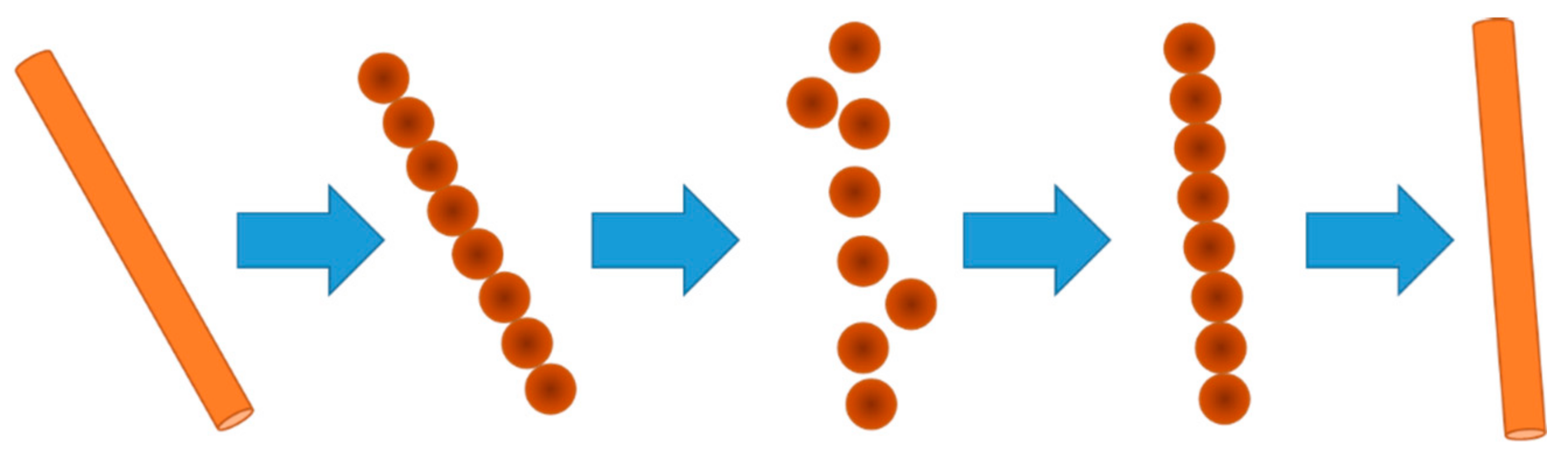
2.1.2. Driftwood Motion Model
- Outline of Driftwood Motion Model
- Bed Friction Terms
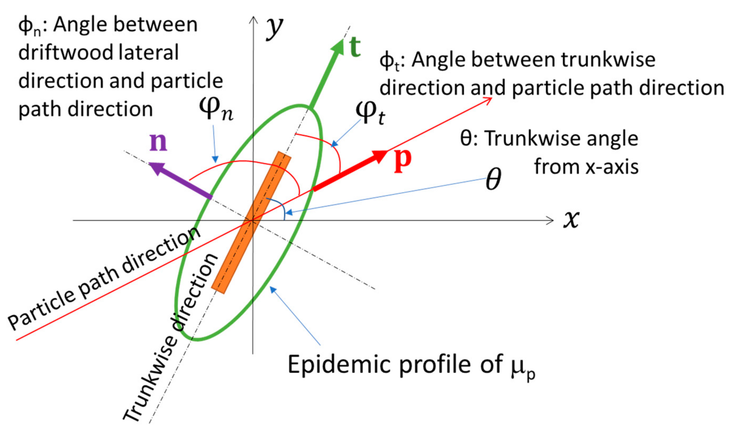
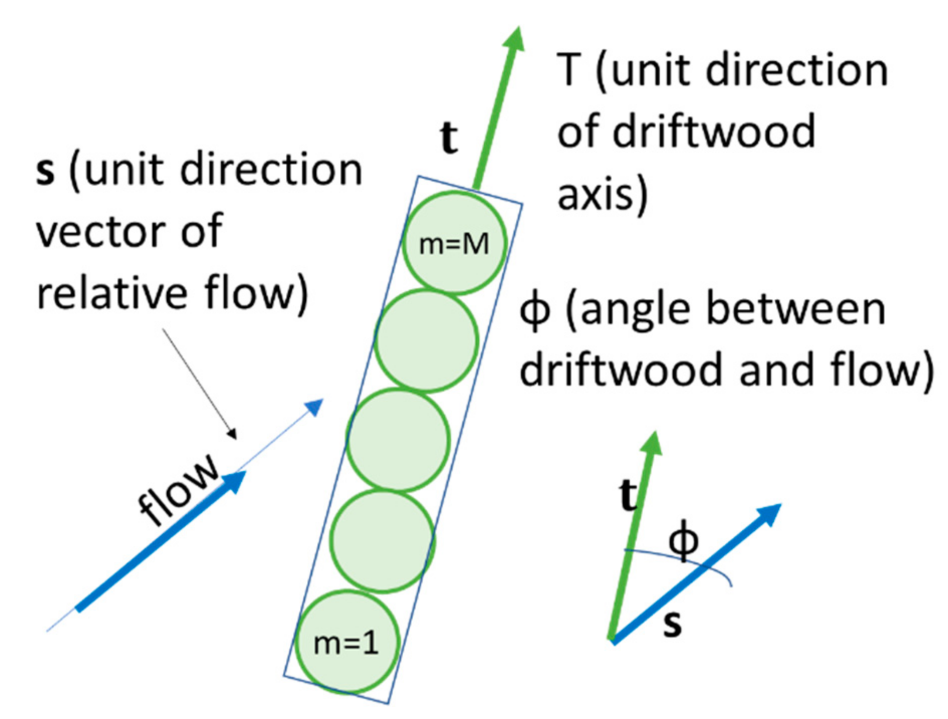
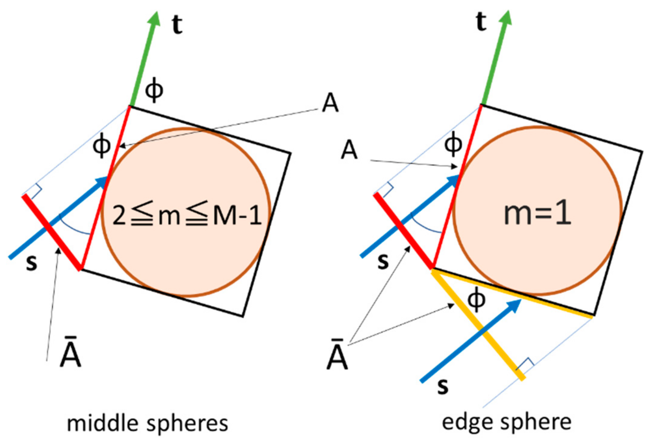
- Drag Force
2.2. Computational Conditions
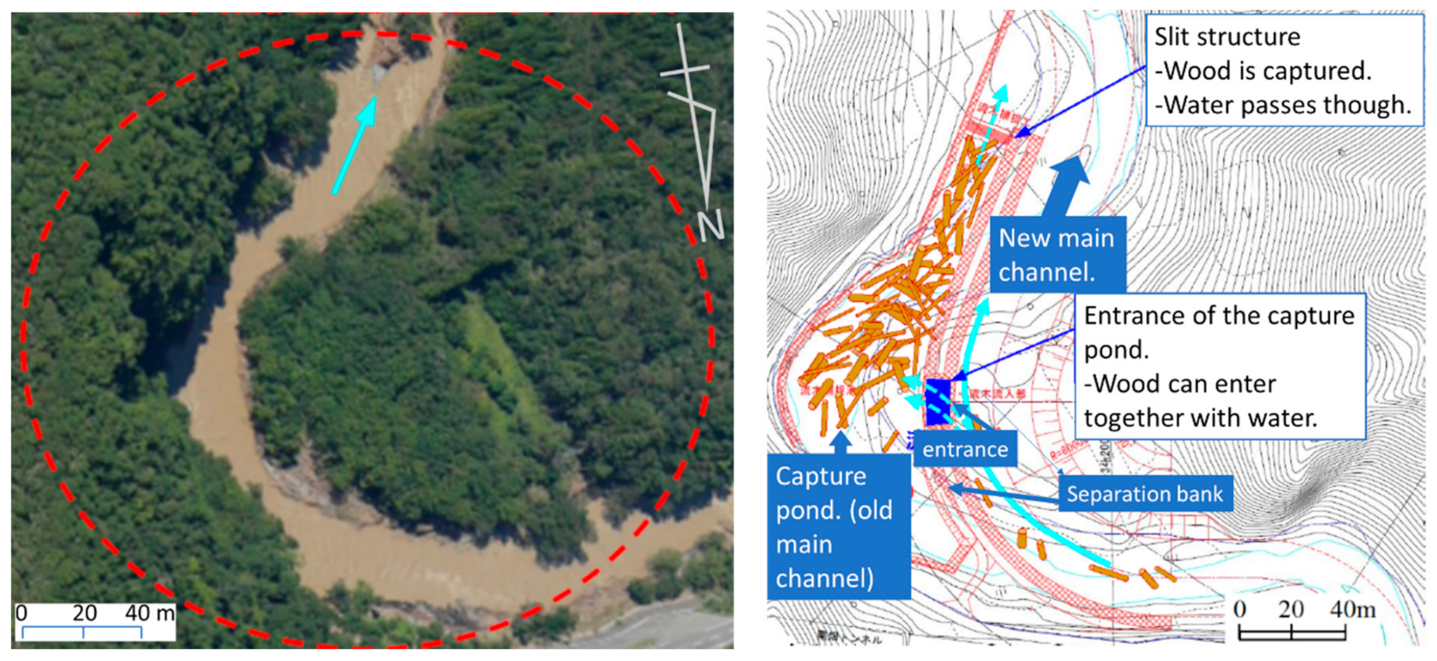
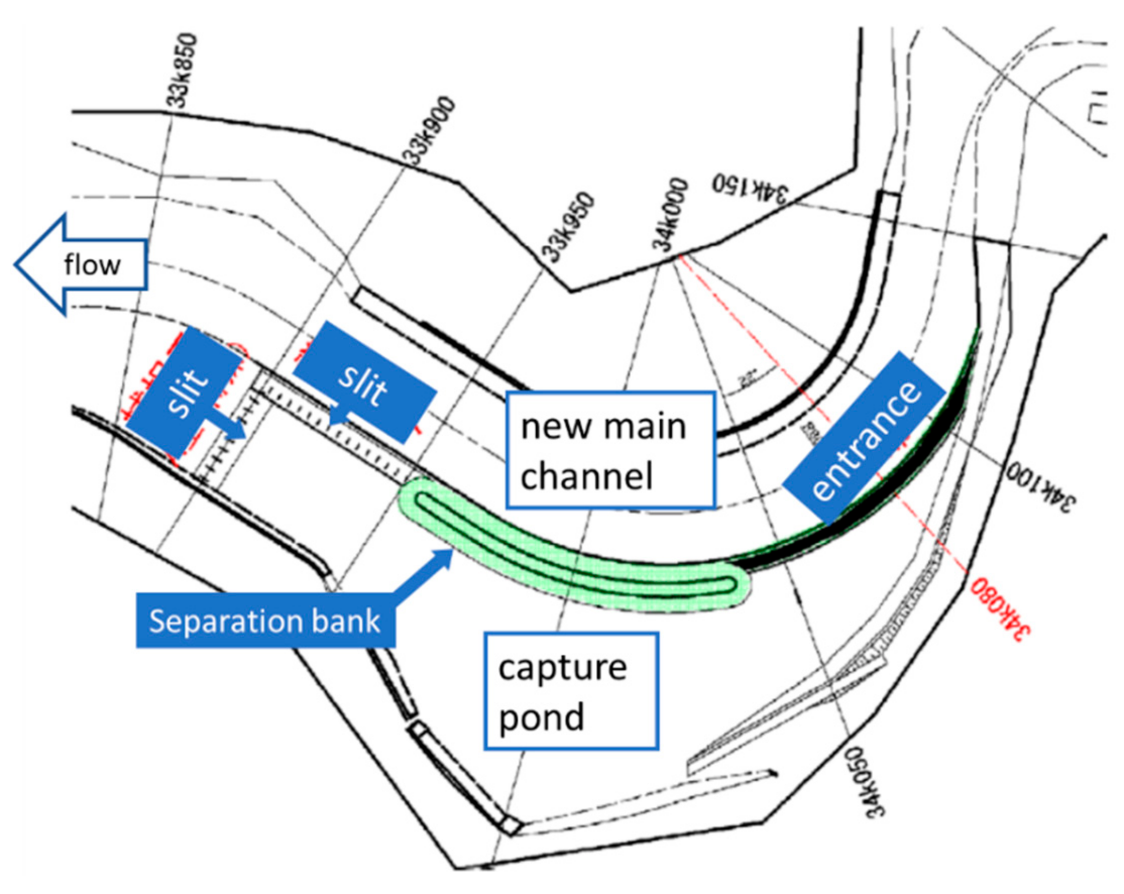
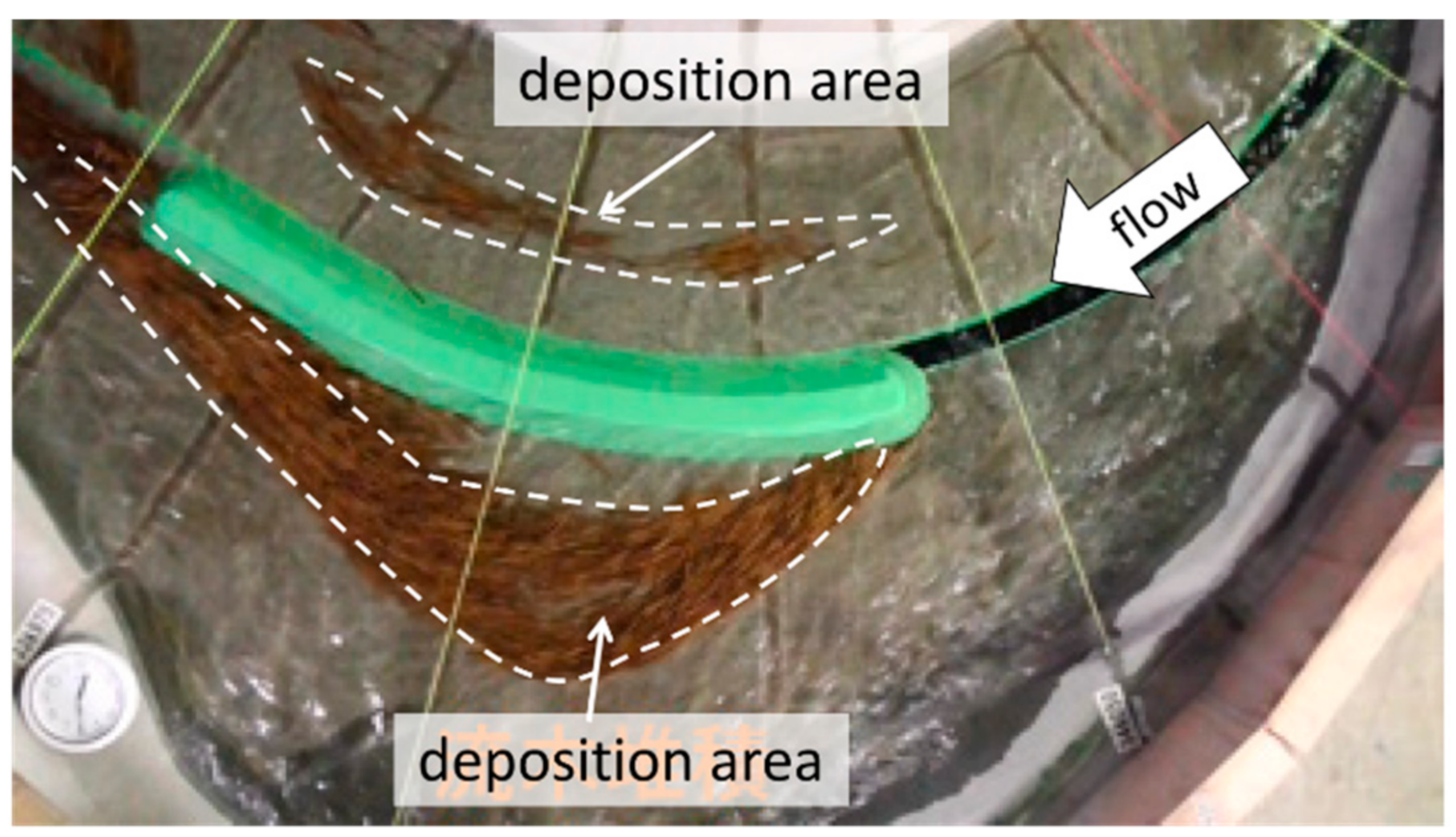
2.2.1. Overview of Laboratory Experiment Performed by Kato et al.
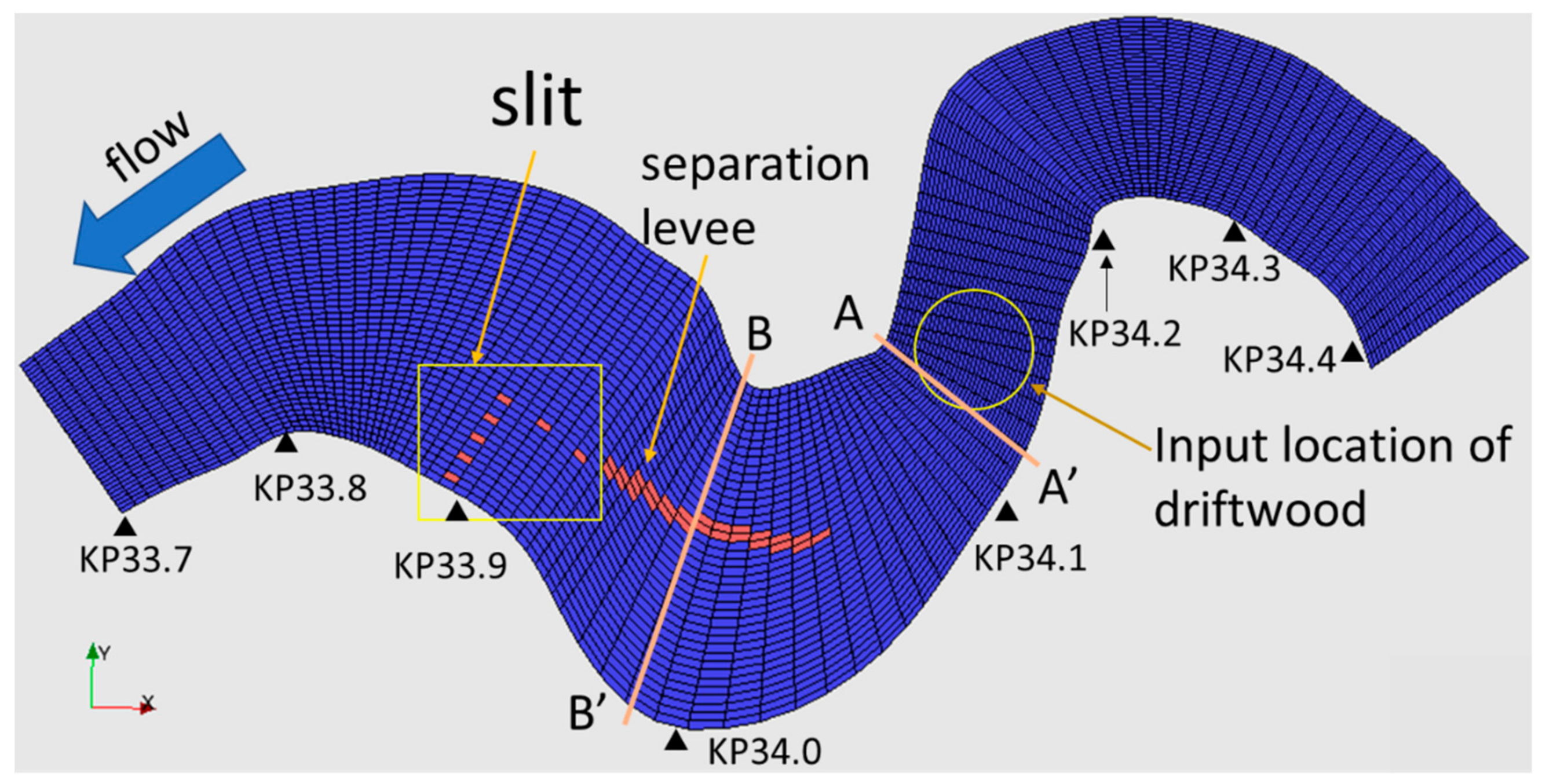
2.2.2. Computational Conditions
3. Results
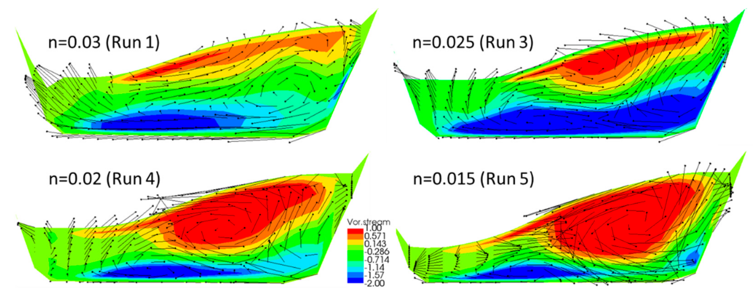
3.1. Cross-Sectional Flow Pattern
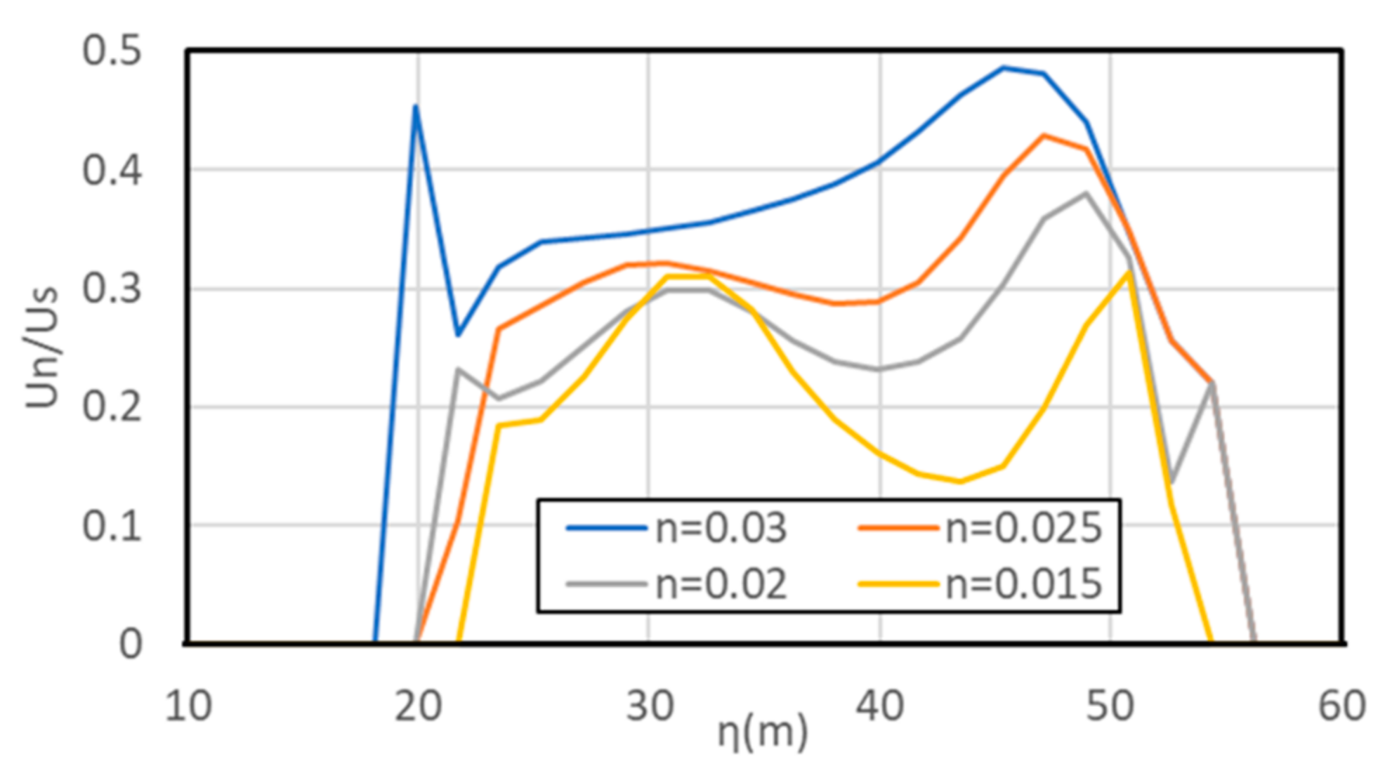
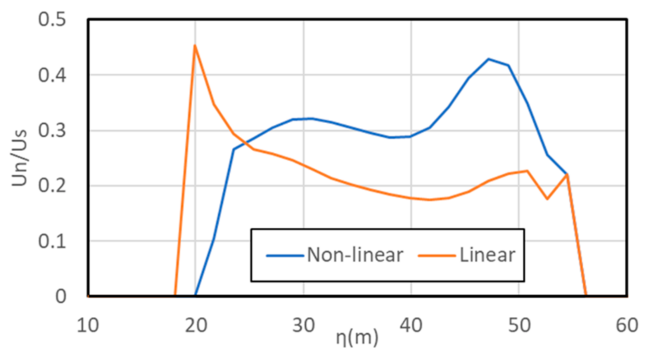
3.2. Strength of Secondary Current
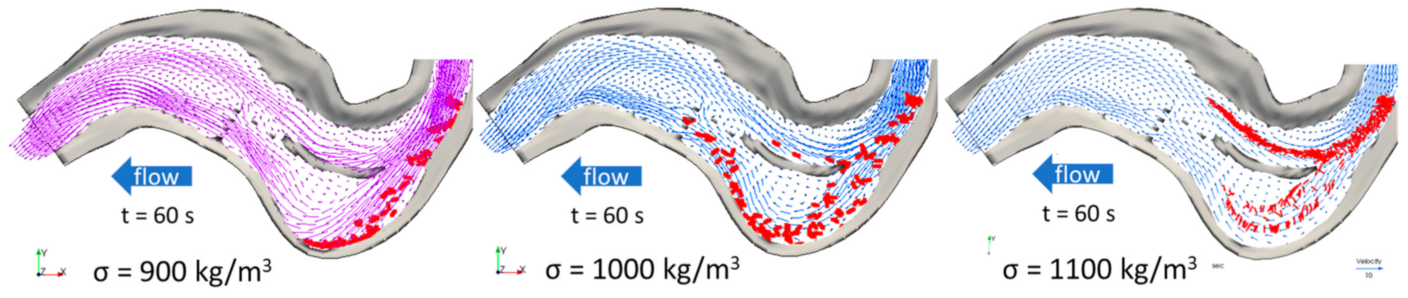
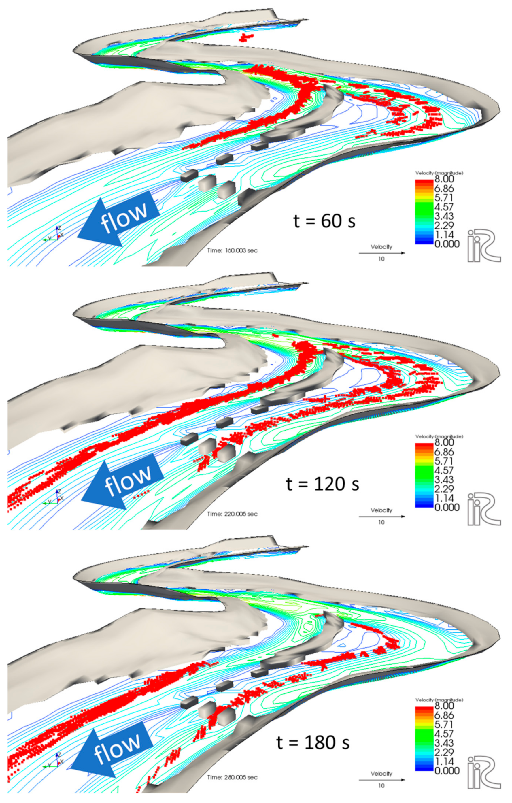
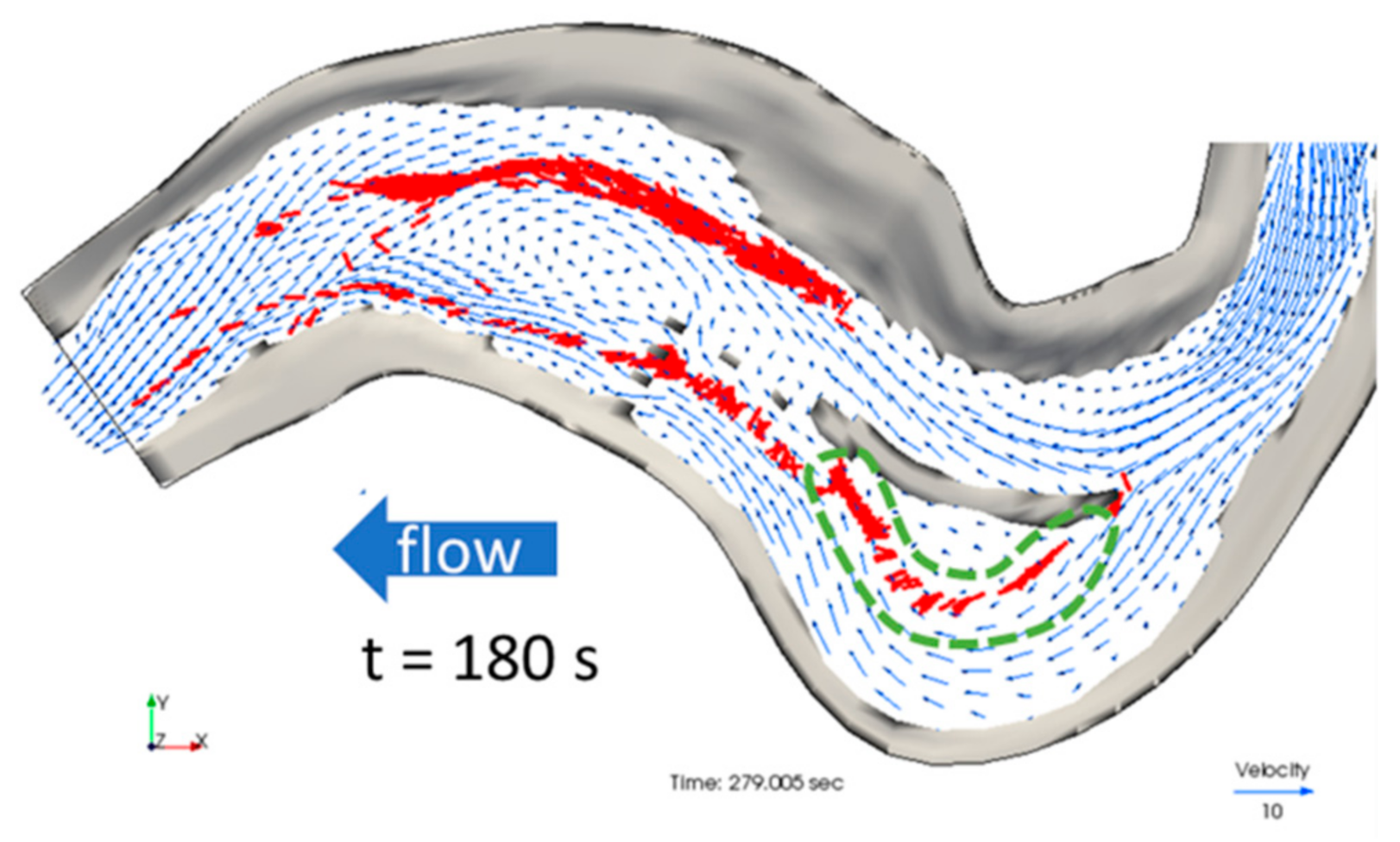
3.3. Driftwood Behavior
3.4. Driftwood Capture Ratio
4. Discussion
4.1. Reproducibility of Basic Characteristics of Driftwood Behavior
4.2. Effect of Manning Roughness Coefficient
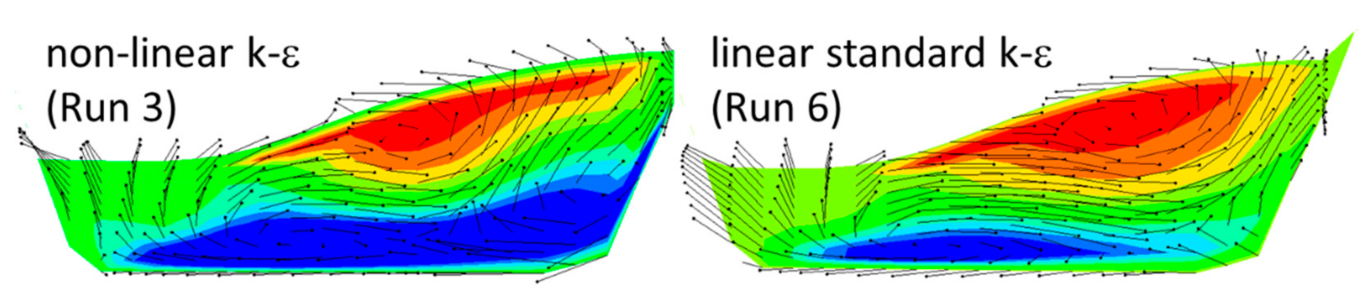
4.3. Effect of Turbulence Model
4.4. Effect of Vertical Grid Division
4.5. Effect of Wood Density
5. Conclusions
Author Contributions
Funding
Conflicts of Interest
References
- Schmocker, L.; Weitbrecht, V. Driftwood: Risk Analysis and Engineering Measures. J. Hydraul. Eng. 2013, 139, 683–695. [Google Scholar] [CrossRef]
- Okamoto, T.; Sanjou, M.; Kashihara, Y. Experimental study on driftwood capturing system using retarding basin. J. Jpn. Soc. Civ. Eng. B1 (Hydraul. Eng.) 2018, 74, 673–678. [Google Scholar] [CrossRef]
- Kato, K.; Ogasawara, T.; Matsubayashi, Y.; Watanabe, K.; Miura, T.; Kanno, T.; Yamaguchi, S.; Watanabe, Y.; Aakahori, R.; Chiba, K. Experimental study on design of driftwood capturing facility in Omoto River, Advances in river engineering. JSCE 2018, 24, 137–142. [Google Scholar]
- Ruiz-Villanueva, V.; Bladé, E.; Sánchez-Juny, M.; Marti-Cardona, B.; Díez-Herrero, A.; Bodoque, J.M. Two-dimensional numerical modeling of wood transport. J. Hydroinform. 2014, 16, 1077–1096. [Google Scholar] [CrossRef]
- Ruiz-Villanueva, V.; Gamberini, C.; Bladé, E.; Stoffel, M.; Bertoldi, W. Numerical Modeling of Instream Wood Transport, Deposition, and Accumulation in Braided Morphologies Under Unsteady Conditions: Sensitivity and High-Resolution Quantitative Model Validation. Water Resour. Res. 2020, 56. [Google Scholar] [CrossRef]
- Kang, T.; Kimura, I.; Shimizu, Y. Numerical simulation of large wood deposition patterns and responses of bed morphology in a braided river using large wood dynamics model. Earth Surf. Process. Landf. 2020, 45, 962–977. [Google Scholar] [CrossRef]
- Kang, T.; Kimura, I.; Onda, S. Application of Computational Modeling for Large Wood Dynamics with Collisions on Moveable Channel Beds. Adv. Water Resour. 2021, 152, 103912. [Google Scholar] [CrossRef]
- Persi E, Petaccia G, Sibilla S, Brufau P, García-Navarro P. Calibration of a dynamic Eulerian-lagrangian model for the com-putation of wood cylinders transport in shallow water flow. J. Hydroinform. 2019, 21, 164–179. [Google Scholar] [CrossRef]
- Shimizu, Y.; Osada, K. Numerical experiments on accumulation process of driftwoods around piers by using a dem-flow coupling model. Proc. Hydraul. Eng. 2007, 51, 829–834. [Google Scholar] [CrossRef] [Green Version]
- Hatta, N.; Akahori, R.; Shimizu, Y. Experimental study and numerical analysis on field on meandering channel and movement of woody debris. J. Jpn. Soc. Civ. Eng. Ser. A2 (Appl. Mech. (AM)) 2012, 68, I_415–I_422. [Google Scholar] [CrossRef] [Green Version]
- Osada, K.; Shimizu, Y. Development of numerical analysis method for driftwoods behavior with bending deformation. J. Jpn. Soc. Civ. Eng. Ser. B1 (Hydraul. Eng.) 2018, 74, I_763–I_768. [Google Scholar] [CrossRef]
- Kimura, I.; Kitazono, K. Effects of the driftwood Richardson number and applicability of a 3D–2D model to heavy wood jamming around obstacles. Environ. Fluid Mech. 2019, 20, 503–525. [Google Scholar] [CrossRef]
- Kato, K.; Sumner, T.; Miura, T.; Kanno, T.; Chiba, K.; Inoue, T.; Shimizu, Y. Numerical Analysis on the Behavior of Driftwood in Driftwood Capturing Facility. J. Jpn. Soc. Civ. Eng. Ser. B1 (Hydraul. Eng.) 2019, 75, I_1441–I_1446. [Google Scholar] [CrossRef]
- Engelund, F. Flow and Bed Topography in Channel Bends. J. Hydraul. Div. 1974, 100, 1631–1648. [Google Scholar] [CrossRef]
- Kimura, I.; Onda, S.; Hosoda, T.; Shimizu, Y. Computations of suspended sediment transport in a shallow side-cavity using depth-averaged 2D models with effects of secondary currents. HydroResearch 2010, 4, 153–161. [Google Scholar] [CrossRef]
- Uchida, T.; Fukuoka, S. Numerical calculation for bed variation in compound-meandering channel using depth integrated model without assumption of shallow water flow. Adv. Water Resour. 2014, 72, 45–56. [Google Scholar] [CrossRef]
- Kimura, I. 3D computations on driftwood jamming around bridge piers. J. Jpn Soc. Civ. Eng. B1 (Hydraul. Eng.) 2019, 75, 601–606. [Google Scholar] [CrossRef]
- Kang, T.; Kimura, T. Computational modeling for large wood dynamics with root wad and anisotropic bed friction in shallow flows. Adv. Water Resour. 2018, 121, 419–431. [Google Scholar] [CrossRef]
- Kang, T.; Kimura, I.; Shimizu, Y. Study on advection and deposition of driftwood affected by root in shallow flows. J. Jpn. Soc. Civ. Eng. Ser. B1 (Hydraul. Eng.) 2018, 74, 757–762. [Google Scholar] [CrossRef]
- Nelson, J.M.; Shimizu, Y.; Abe, T.; Asahi, K.; Gamou, M.; Inoue, T.; Iwasaki, T.; Kakinuma, T.; Kawamura, S.; Kimura, I.; et al. The international river interface cooperative: Public domain flow and morphodynamics software for education and applications. Adv. Water Resour. 2016, 93, 62–74. [Google Scholar] [CrossRef]
- iRIC Web Site. Available online: http://i-ric.org/en/2020 (accessed on 7 April 2021).
- Kimura, I.; Hosoda, T. A non-linear k–ε model with realizability for prediction of flows around bluff bodies. Int. J. Numer. Method Fluids 2003, 42, 813–837. [Google Scholar] [CrossRef]
- Kimura, I.; Uijttewaal, W.S.J.; Hosoda, T.; Ali, M.S. RANS computations of shallow grid turbulence. J. Hydraul. Eng. 2009, 135, 118–131. [Google Scholar] [CrossRef]
- Kimura, I.; Hosoda, T.; Takimoto, S.; Shimizu, Y. RANS computations on curved open channel flows. J. Hydrosci. Hydraul. Eng. 2009, 27, 29–47. [Google Scholar]
- Suzuki, R.; Kimura, I.; Shimizu, Y.; Iwasaki, T.; Hosoda, T. Numerical study on secondary currents of the second kind in wide shallow open channel flows. In River Flow 2014; Taylor & Francis Group: London, UK, 2014; pp. 179–187. [Google Scholar]
- Schiller, L.; Naumann, Z. A drag coefficient correlation. J. Mod. Phys. 1933, 77, 318–320. [Google Scholar]
- Koshizuka, S.; Oka, Y. Moving particle semi-implicit method: A gridless approach based on particle interactions for incompressible flow simulation. In Proceedings of the 3rd Workshop on Supersimulators for Nuclear Power Plants; University of Tokyo: Tokyo, Japan, 1995; pp. 43–49. [Google Scholar]
- Persi, E.; Petaccia, G.; Fenocchi, A.; Manenti, S.; Ghilardi, P.; Sibilla, S. Hydrodynamic coefficients of yawed cylinders in open-channel flow. Flow Meas. Instrum. 2019, 65, 288–296. [Google Scholar] [CrossRef]


| Type of Friction | Symbol | Value |
|---|---|---|
| Static Friction Coefficient | 2.0 | |
| Sliding Friction Coefficient | 1.0 | |
| Rolling Friction Coefficient | 0.5 |
| Run | Vertical Layer | Turbulence Model | Manning Roughness Coefficient n 1 | Specific Gravity of Wood 2 |
|---|---|---|---|---|
| 1 | 10 | Nonlinear k-ε | 0.03 | 1.1 |
| 2 | 20 | Nonlinear k-ε | 0.03 | 1.1 |
| 3 | 10 | Nonlinear k-ε | 0.025 | 1.1 |
| 4 | 10 | Nonlinear k-ε | 0.02 | 1.1 |
| 5 | 10 | Nonlinear k-ε | 0.015 | 1.1 |
| 6 | 10 | Linear standard k-ε | 0.025 | 1.1 |
| 7 | 10 | Nonlinear k-ε | 0.03 | 1.0 |
| 8 | 10 | Nonlinear k-ε | 0.03 | 0.9 |
| Run | Capture Ratio (%) |
|---|---|
| 1 | 32 |
| 2 | 39 |
| 3 | 59 |
| 4 | 96 |
| 5 | 100 |
| 6 | 88 |
| 7 | 94 |
| 8 | 100 |
| Laboratory experiment | 65~87.5 |
Publisher’s Note: MDPI stays neutral with regard to jurisdictional claims in published maps and institutional affiliations. |
© 2021 by the authors. Licensee MDPI, Basel, Switzerland. This article is an open access article distributed under the terms and conditions of the Creative Commons Attribution (CC BY) license (https://creativecommons.org/licenses/by/4.0/).
Share and Cite
Kimura, I.; Kang, T.; Kato, K. 3D–3D Computations on Submerged-Driftwood Motions in Water Flows with Large Wood Density around Driftwood Capture Facility. Water 2021, 13, 1406. https://doi.org/10.3390/w13101406
Kimura I, Kang T, Kato K. 3D–3D Computations on Submerged-Driftwood Motions in Water Flows with Large Wood Density around Driftwood Capture Facility. Water. 2021; 13(10):1406. https://doi.org/10.3390/w13101406
Chicago/Turabian StyleKimura, Ichiro, Taeun Kang, and Kazuo Kato. 2021. "3D–3D Computations on Submerged-Driftwood Motions in Water Flows with Large Wood Density around Driftwood Capture Facility" Water 13, no. 10: 1406. https://doi.org/10.3390/w13101406
APA StyleKimura, I., Kang, T., & Kato, K. (2021). 3D–3D Computations on Submerged-Driftwood Motions in Water Flows with Large Wood Density around Driftwood Capture Facility. Water, 13(10), 1406. https://doi.org/10.3390/w13101406